Programming and Control of a Single-Column Analog Simulated Moving Bed Process

(1)

Setembro, 2018

João Cabaço Antunes

[Nome completo do autor]

Licenciado em Ciências de Engenharia Química e Bioquímica

[Habilitações Académicas] [Habilitações Académicas] [Habilitações Académicas] [Habilitações Académicas] [Habilitações Académicas] [Habilitações Académicas] [Habilitações Académicas]

Programming and Control of a Single-Column Analog

Simulated Moving Bed Process

[Título da Tese]

Dissertação para obtenção do Grau de Mestre em Engenharia Química e Bioquímica

Dissertação para obtenção do Grau de Mestre em [Engenharia Informática]

Orientador: José Paulo Barbosa Mota, Professor Catedrático, FCT-UNL Co-orientadores: Tiago Santos, Doutorando, FCT-UNL

Júri:

Presidente: Dr. Joaquim Silvério Marques Vital

Arguentes: Dr. Mário Fernando José Eusébio

(2)

(3)

Programming and Control of a Single-Column Analog Simulated Moving Bed Process

A Faculdade de Ciências e Tecnologia e a Universidade Nova de Lisboa têm o direito, perpétuo e sem limites geográficos, de arquivar e publicar esta dissertação através de exemplares impressos reproduzidos em papel ou de forma digital, ou por qualquer outro meio conhecido ou que venha a ser inventado, e de a divulgar através de repositórios científicos e de admitir a sua cópia e distribuição com objetivos educacionais ou de in-vestigação, não comerciais, desde que seja dado crédito ao autor e editor.

(4)

(5)

i "Those who brave the thorn may eat the rare fruit." -Conclave Master Tesshin.

(6)

(7)

iii Acknowledgements

I would like to express my sincere gratitude to my Prof. Paulo Mota for the contin-uous support of my study and work, for his patience and immense knowledge. I’d also like to extend this thanks to Tiago Santos and Abimaelle Chibério for aiding me in the development and use of my developed work. Furthermore, I’d also like to show appreci-ation towards my colleague Gonçalo Policarpo, who has worked with me along with his own master thesis.

Finally, I’d like to give thanks to my family, my parents for their immense patience and my brother for helping me with the writing of this thesis.

(8)

(9)

v

Abstract

With the advancements in technology, the development of tools for the control and testing of the progress in different fields, such as chromatography, has become essential in concerns to lab work and prototyping. As such, many programming languages have been adapted and developed with the objective to make the development of such tools easier.

As our group built the Single-Column Analog Simulated Moving Bed chromatog-raphy process, the need for a versatile program to ease and simplify the procedure of tests and adjustments was met with the development of a tool written in the Julia and Python programming languages. The use of the aforementioned languages enabled us to speed up the processes of testing and modifying the system built, helping us to get more accurate results and meet deadlines for reports and presentations.

With this it can be summarized that the development of easy-to-use programs aided by effective programming languages for the purpose of technological and scientific re-search is of the interest of various different fields as it allows them to hasten the develop-ment of the processes in study.

Keywords: Programming, Computer Science, Chromatography, Simulated Mov-ing Bed

(10)

(11)

vii

Resumo

Com os avanços em tecnologia, o desenvolvimento de ferramentas para o controlo e teste no progresso em diferentes áreas, como a cromatografia, tem sido essencial em termos de trabalho laboratorial e criação de protótipos. Com isto, várias linguagens de programação foram adaptadas e desenvolvidas com o objetivo de facilitar o desenvolvi-mento de tais ferramentas.

À medida que o nosso grupo construiu o processo de cromatografia de Leito Móvel Simulado de Coluna Única, a necessidade de um programa versátil para facilitar e sim-plificar o procedimento de testes e ajustes foi satisfeita no desenvolvimento de uma fer-ramenta escrita nas linguagens de programação Julia e Python. O uso das linguagens acima mencionadas permitiu-nos acelerar os processos de teste e modificação do sistema construído, ajudando-nos a obter resultados mais precisos e cumprir prazos para relatórios e apresentações.

Com isto, pode-se sumarizar que o desenvolvimento de programas fáceis de usar com auxílio a linguagens de programação eficazes para fins de pesquisa científica e tec-nológica é do interesse de vários campos diferentes, pois permite acelerar o desenvolvi-mento dos processos em estudo.

(12)

(13)

ix

List of Figures

Figure 1 - Priciple of Elution Chromatography. ... 1

Figure 2 - Diagram of a True Moving Bed. ... 2

Figure 3 - Diagram of a Simulated Moving Bed. ... 3

Figure 4 - Schematic diagram of the Single Column Setup. ... 4

Figure 5 - Schematic of the Single Column chromatographic process with recycle lag, analogous to a four-zone SMB. ... 5

Figure 6 - Logo for the Julia language. ... 8

Figure 7 - Logo for the Python language... 9

Figure 8 - Diagram of the setup with pumps, seven two-way valves, the two 2 position valves and spectrometer connected (although the image shows two only the UV2 spectrometer is connected). ... 12

Figure 9 - The Valco 2-position valve (right) with and actuator module (top left) and a manual controller (bottom left). ... 13

Figure 10 - Example of the graph obtained through the use of python's matplotlib package using data from oo_spectrometer.jl, the top graph represents the intensity (in red) and absorbance (in blue) measured by the spectrometer moment to moment while the bottom graph presents the absorbance of the selected wavelength along time. ... 38

Figure 11 - Hierarchical diagram of each developed program. ... 43

Figure 12 - Mockup of the user interface designed for the ChromatographyStudio.jl program. ... 45

(16)

(17)

xiii

List of Tables

Table 1 - The different commands to set the pump's parameters and values and examples of their

usage. ... 16

Table 2 - The different commands to get information from the pump's parameters and examples of their usage. ... 17

Table 3 - The different commands to use the scale through serial connection... 18

Table 4 - The different commands to set the valve's parameters and values. ... 19

Table 5 - The different commands to get information from the valve's parameters... 19

Table 6 - The different commands and their respective decimal and hexadecimal values to set the relay states on each board. ... 20

Table 7 - The different commands and their respective decimal and hexadecimal values to get information about the relay states on each board. ... 21

(18)

(19)

1

1- Introduction to Chromatography

Chromatography is a separation and analytical technique initially developed by chemists with the goal of extraction and purification of mixtures of plant origin. Its name originates from the Greek, to write colors.

Chromatography is a separation method in which a mixture of solutes is eluted through a stationary phase (usually a solid inside a column), with each compound inter-acting with the solid. The affinity that each solute has with the stationary phase will de-termine their migration speeds, enabling the collection of separated compounds based on how strongly they interact with the stationary phase. A strong affinity towards this phase will lead towards slower migration speeds of compounds, while compounds with lower affinities elute more quickly, as can be seen in Figure 1.

Figure 1 - Priciple of Elution Chromatography.

(20)

2

1.1 Development of the Simulated Moving Bed process

In an attempt to improve the described process, the True Moving Bed process was developed, employing unique operating principles and conferring a number of valuable benefits to the chromatographic separation process. The process changes how the solid phase operates, no longer being immovable, it starts to have a continuous movement, countercurrent to the flow of the fluid and with an intermediate velocity in relation to the migration speed of the two solutes to be separated. As the compound that interacts most strongly with the phase (named the extract) will be dragged by the solid, the other (named the raffinate) continues to migrate with the fluid but at a lower speed. With this, it is possible to collect each pure compound in each end of the column, allowing for the con-tinuous feed of mixture to be separated [1], as can be understood with Figure 2.

Figure 2 - Diagram of a True Moving Bed.

However, the True Moving Bed process has been difficult to implement, as it relies on a continuous flow of eluent in one direction being recycled back into the column filled with a chromatographic medium, and a continuous flow of said medium circulating in countercurrent to the eluent and also being recycled. This results in problems such as friction of particles in the bed and not being economically viable.

(21)

3 As a mean to overcome some of the True Moving Bed process’s shortcomings, Universal Oil Products developed the Simulated Moving Bed process in 1961. Essentially being the discretization of the True Moving Bed in several columns (the higher the num-ber of columns, the closer the Simulated Moving Bed process becomes to the True Mov-ing Bed process), simulatMov-ing the opposMov-ing currents by periodically shiftMov-ing the inlets/out-lets ports in the direction of the fluid flow [2], as demonstrated in Figure 3.

Figure 3 - Diagram of a Simulated Moving Bed.

In its conventional operating mode, at regular time intervals, the designated injec-tion and withdrawal ports all move one secinjec-tion ahead in the direcinjec-tion of the fluid flow. When the initial injection/collection port of all the streams is reached, we have completed one cycle. In this way, during one cycle the same column is being used towards different roles in the separation process.

(22)

4 With this and the interest of adapting this process to other industries and applica-tions, the Simulated Moving Bed technology was advanced upon and scaled down, with more versatile configurations with reduced size and number of columns being preferred, creating an alternative to the use of the initial process arrangement where several columns with large dimensions were employed.

This developmental trend is supported by an increase in complexity, which in most cases requires highly versatile equipment, advanced optimization and modelling tools and robust control methods, although still presenting the advantages of having an increased throughput, purity, and yield relative to batch chromatography and reduction in eluent consumption.

1.2 Development of the Single Column Analog process

The Single Column Analog process, illustrated in Figure 4, was developed with the increased efficiency of methods to model the periodic state of the analogous multi-col-umn process in mind, reducing the set of equations needed to describe the process from various columns to a single one [1].

Figure 4 - Schematic diagram of the Single Column Setup.

This process has been shown to substantially decrease the amount of solute and mobile phase needed to proceed with the Simulated Moving Bed process, as well as being an economic and optimal method of testing a set of operating conditions for new multi-column chromatographic separation procedures [3].

(23)

5

Figure 5 - Schematic of the Single Column chromatographic process with recycle lag, analogous to a four-zone SMB.

In this sense, the present thesis presents the development of a custom program, denominated ChromatographyStudio.jl, for control, testing and data acquisition of the Single Column Analog setup illustrated in Figure 5, simplifying its operation and facili-tating the adjustment of several setup parameters.

(24)

(25)

7

2- Programming Languages

2.1 High-level programming languages

A high-level programming language is a type of programming language that has strong degree of abstraction from the basis of the computer, in contrast to low-level programming languages. It is usually composed of more natural language use and terms, easy to use and may automate significant areas of computing systems, making the process of developing a program simpler and more understandable than when using a lower-level language at the cost of effi-ciency. Some examples of high-level programming languages include Fortran, Visual Basic and C#.

2.2 Programming Languages Used

Julia

Julia, identified by its logo in Figure 6, is a free high-level dynamic programming lan-guage developed by Jeff Bezanson, Stefan Karpinski, Viral B. Shah, and Alan Edelman and first made available in 2012. Originally designed to address the needs of high-performance numerical analysis and computational science, it was developed for the use in scientific pur-poses as it includes a differential equations ecosystem, optimization tools, iterative linear solv-ers and simplification and aid with data interaction and interpretation. All this contained in efficient libraries for floating-point calculations and linear algebra[4].

(26)

8 Of note is the existence of JuliaCon, an academic conference for Julia users and devel-opers, held annually since 2014, furthering denoting the commitment of developing the lan-guages towards academia and the use of the Julia language by the Federal Reserve Bank of New York to model the United States economy, achieving a model estimation time nearly 10 times faster than the previously used language, MATLAB [5].

Figure 6 - Logo for the Julia language.

Of the multitude of tools offered by the Julia library, this thesis focuses on the use of the following packages:

• PyCall.jl - This package provides the ability to directly call and operate with the Python language from the Julia language, enabling the arbitrary import of Python modules from Julia, call of Python functions, definition of Python classes from Julia methods and sharing large data structures between Julia and Python without copying them [6].

• PyPlot.jl - Used with the PyCall package, this module provides a Julia interface to the Matplotlib plotting library from Python [7].

• PySerial.jl - Used with the PyCall package, this module provides a Julia interface to the PySerial module from Python, enabling access for the serial ports present on the computer [8].

• SerialPorts.jl - Used with the PySerial package, this module simplifies the serial communication with different devices through Julia, mimicking regular file in-put/output as in the Base Julia library [9].

• Gtk.jl – This module is an iteration of the GIMP Toolkit, designed for the creation graphical user interfaces, implemented in Julia [10].

(27)

9

Python

Python, with its logo represented in Figure 7, is a free high-level programming language developed for general-purpose programming by Guido van Rossum and released in 1991. Its design philosophy accentuates code readability as it provides constructs that enable clear pro-gramming on both small and large scales, featuring automatic memory management and sup-porting various programming paradigms. Due to its longevity and widespread use, the Python language has also developed a vast and wide-ranging library.

Figure 7 - Logo for the Python language.

This thesis focuses on the use of the following packages:

• Matplotlib - A Python 2D and 3D plotting library which produces publication quality figures heavily inspired and based on MATLAB’s plotting functions. • PySerial – This module encapsulates the access to the serial ports present [11]. • Python-seabreeze – A SeaBreeze library wrapper developed independently from

Ocean Optics, used to communicate with the spectrometer [12].

2.3 Programming Paradigms Followed

To develop this program the Julia language was used as the main programming envi-ronment due to its flexible and versatile implementation of object-oriented programming and parallel computing.

The main structure of the program is composed of a central module that calls upon other different modules to define the functions needed for the automation of the Single-Column An-alog Simulated Moving Bed process, with the lowest level of modules being composed of driv-ers designed to facilitate the interaction between each instrument and the computer in parallel with each other.

(28)

10 To achieve this, the base drivers are composed of two main parts:(1) defining a new data type for the instrument it’s controlling and (2) defining the functions that will control said instrument according to its manual or protocol. By doing this each instrument is represented by a data type with its own attributes and functions.

In general, the mentioned functions will be used to either get information from the in-strument, for example reading the weight measured by a scale, or set the instrument’s operating parameters, such as the flowrate of a pump.

This approach allows for the program to be highly customizable to adaptive to the in-struments implemented in the setup as, when adding new inin-struments, there is only a need to certify that said instrument works with the same protocol previously implemented and then represent it with the data type created for this purpose. For example, pumps from the same manufacturer might use the same means of communication with the computer and, as such, adding several pumps with the same communication protocol would only need to add a few lines of code to represent the additions as variables ready to be controlled.

(29)

11

3- Instruments and Setup

3.1 Instruments used in the process

To proceed with the Single-Column Analog setup, the instruments needed for the digital control of the process are the following:

• A Knauer V5010 S100 Smartline pump; • Two Knauer WellChrom HPLC K501 pumps; • Two Robot Electronics OptoRLY88 relay boards; • Two VICI Valco 2-position valves;

• A Sartorius TE3102S weight scale; • An OceanOptics USB2000 Spectrometer.

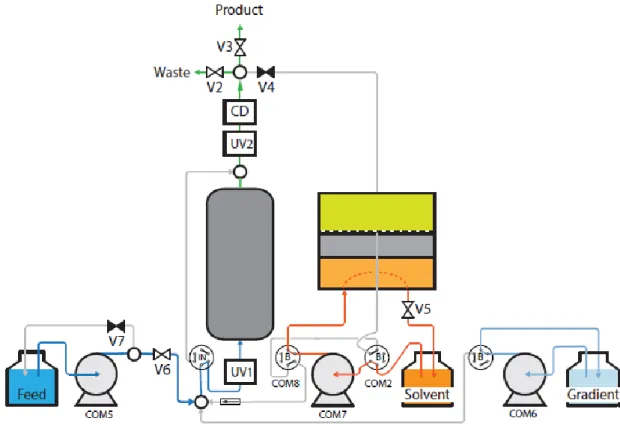
All these instruments are connected to a single computer running the custom software developed by this thesis and make up the system necessary for the Single-Column Analog pro-cess, shown in Figure 8 and in Annexes 2 through 8.

The three pumps present (the single Smartline pump and the two K501 pumps) are used to run the process, with the Smartline pump, denominated Pump F, used for the feeding of the process, one of the K501 pumps, denominated Pump E, responsible for the elution of the sep-arating mixture and the last K501 pump, denominated Pump G, used for developing concen-tration gradients in the process. Worth mentioning is that, although it was not used during ex-perimental tests, Pump G is still capable of being controlled through the developed software.

The two OptoRLY88 relay boards are used to signal the pneumatic actuators of the dif-ferent valves of the setup.

(30)

12 The two Valco 2-position valves are used in the port switching action needed for the execution of the Simulated Moving Bed process.

A TE3102S weight scale is used to measure the amount of raffinate and extract yielded during the separation process.

The OceanOptics USB2000 Spectrometer is used to measure the purity of the flowing fluid.

Figure 8 - Diagram of the setup with pumps, seven two-way valves, the two 2 position valves and spectrometer connected (although the image shows two only the UV2 spectrometer is

connected).

3.2 The Setup

The various instruments in the setup require different types of connectors.

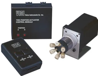
The pumps and the scale use a RS232 type connector to connect directly to the computer, with the Valco 2-position valves needing an actuator control module to be connected in the same way (the computer being connected to the actuator through a RS232 serial port connec-tion and the actuator being connected to the 2-posiconnec-tion valve via a VICI proprietary motor driver output cable), as can be seen in Figure 9.

(31)

13

Figure 9 - The Valco 2-position valve (right) with and actuator module (top left) and a manual controller (bottom left).

Worth mentioning is the use of a MOXA 8 Ports Serial PCI Express controller card PCI-e to multi RS232 DB9 Ports convPCI-ertPCI-er I/O card installPCI-ed on thPCI-e computPCI-er to PCI-enablPCI-e thPCI-e com-munication with the five RS232 connectors.

The rest of the instruments, the two OptoRLY88 relay boards and the USB2000 Spec-trometer, are connected via a USB 2.0 B connector.

(32)

(33)

15

4- Development of individual drivers

4.1 Controlling the different instruments

The first step in the development of the controlling software is the creation of preliminary drivers for each type of instrument. In the case of most of the equipment in use, the writing of such drivers can occur based on the device’s manual information on external control via serial communication, however, in the case of the OceanOptics Spectrometer, the independently de-veloped Python-seabreeze python package is used, as the only method of use for this instrument made available by the manufacturer is through a C/C++ based device driver or through their proprietary OOIBase32 Spectrometer Operating Software.

Pumps

The Knauer V5010 S100 Smartline and WellChrom HPLC K501 pumps’ share identical external control protocols, which are as follows:

The specifications for data transfer are a baud rate of 9600, 8 bits of data with 1 stop-bit and no parity check.

A list of simple ASCII codes is able to control the pump, encoding the different com-mands available to the user.

After each successful command transfer, the message “OK” will be sent back from the pump. Inadmissible commands are answered by a question mark “?”. Each command and each answer must be confirmed using a carriage return (ending the command string in “\r”).

(34)

16

Table 1 - The different commands to set the pump's parameters and values and examples of their usage.

ASCII

Command Description Example of the command

Fxxxx Sets the flow rate to xxxx μL/min. “F200\r” Sets the pump flow rate to 200 μL/min.

M1 Starts the pump, using the

cur-rently selected flow rate. “M1\r”

The pump starts pumping fluid at the set flow rate (this can include 0 μL/min.

M0 Stops the pump. “M0\r” Stops the pump from pumping.

S1 Enables both manual (with the

keypad) and serial control. “S1\r”

The pump can be controlled via its keypad or through commands given through a serial connection.

S0

Disables manual control (only the STOP key is active), while still permitting serial control.

“S0\r”

The pump can only be controlled through the serial connection, with the only key being active being the STOP in case of the need to the pump.

Pxxx.xxx

Set maximum pressure threshold , in MPa, for automatic pump cut-off.

“P200.000\r ”

Sets the maximum pressure threshold to 20 MPa.

pxxx.xxx

Set minimum pressure threshold , in MPa, for automatic pump cut-off.

“p010.000\r ”

Sets the minimum pressure threshold to 10 MPa, the pump cuts-off, if this threshold is not attained for a period of 60 seconds.

(35)

17

Table 2 - The different commands to get information from the pump's parameters and exam-ples of their usage.

ASCII Command Description Example of the command

P?

Current system pressure in-quiry replied with

“Pxx.xxx”.

“P?\r”

The pump replies with

“P15.000”, indicating a pressure of 15 MPa.

S? Pump status inquiry. “S?\r”

The reply will contain two bytes in binary form. The first is the status byte and shows the motor status in bit 4 (1=ON; 0=OFF). The second one shows the last er-ror code (0=no erer-ror; 1=motor blocked; 2=stop via the keypad), which will then be automatically deleted.

T? Pump model inquiry. “T?\r”

The pump replies with 16 charac-ters identifying the pump model, e.g. KNAUER MICROPUMP

V? Program version inquiry. “V?\r”

The pump replies with the current version of the program its run-ning, e.g. V1.24F

Weight Scale

The Sartorius TE3102S weight scale’s external control protocols are as follows:

The specifications for data transfer can be defined in the scale’s menu, with the specifi-cations in use for this project being a baud rate of 9600, 7 bits of data with 1 stop-bit and an odd parity.

A list of simple ASCII codes is able to control the scale, encoding the different commands available to the user.

Each command sent and must be must start with the ESC character (starting each com-mand string with”\x1b”) and optionally end with a carriage return and line feed (ending the command string in “\r” or “\n” respectively, or “\r\n” using both).

The total length of a command is anywhere from 4 total characters (with 1 command character between the start and end described above) to 7 total characters (with a maximum of 4 com-mand characters).

(36)

18

Table 3 - The different commands to use the scale through serial connection.

Command Character Function Example of the command K Changes the scale’s weighing mode

to mode 1. ”\x1bK\r” L Changes the scale’s weighing mode

to mode 2. ”\x1bL\r” M Changes the scale’s weighing mode

to mode 3. ”\x1bM\r” N Changes the scale’s weighing mode

to mode 4. ”\x1bN\r”

O Blocks the use of the keys. ”\x1bO\r”

P

The scale replies with a reading ac-cording to the output format (see

Annex I) to the serial port.

”\x1bP\r”

R Enables the use of the keys. ”\x1bR\r”

S Restarts the scale. ”\x1bS\r”

T Tares and zeros the scale. ”\x1bT\r”

U Only tares the scale. ”\x1bU\r”

V Only zeros the scale. ”\x1bV\r”

W Provide external calibration

(de-pending on menu settings). ”\x1bW\r”

2-position Valves

The VICI Valco 2-position valves are controlled via a connection to a proprietary actua-tor. Its external control protocols are as follows:

The specifications for data transfer are a baud rate of 9600, 8 bits of data with 1 stop-bit and no parity check.

A list of simple ASCII codes is able to control the actuator, defining the commands the actuator will send to the valve.

(37)

19 Each command sent and must be terminated with a carriage return (ending the command string in “\r”). Of note is that line feed characters (“\n”) sent to the device will be ignored.

Table 4 - The different commands to set the valve's parameters and values.

Commands Function

GOa Sends actuator to position a, where a is either position A or B. CW Sends actuator to position A.

CC Sends actuator to position B.

TO Toggles actuator to the opposite position.

TT Toggles actuator to the opposite position, waits a set delay time, then tog-gles it back to the original position.

DTx Sets the delay time, in milliseconds, where x can be an integer between 0 and 65 535.

IDx Sets the device ID to x, where x can be an integer between 0 and 9. SBx Sets the baud rate to x, where x can be between 2 400 and 115 220, with a

default setting of 9600.

SMx Sets the digital input mode to x, where x can be an integer between 1 and 4.

SOx

Sets the delay time before the position outputs are turned off to the closest 5 millisecond interval to x, where x can be an integer between 0 and 30 000. The outputs are always on (SO=0) by default.

CNTx Sets the move count to x, where x can be an integer between 0 and 65 000. IN Starts an initialization sequence.

Table 5 - The different commands to get information from the valve's parameters.

(38)

20 VR The actuator replies with the part number and date of the firmware. CP The actuator replies with the current actuator position.

GV The actuator replies with the measured DC input voltage.

GVD The actuator replies with the measured DC input voltage drop while moving.

? The actuator replies with a list of valid commands.

Relay Boards

The two Robot Electronics OptoRLY88 relay boards are both connected via a USB 2.0 B connector. However, because it is connected directly to the processor, the relay boards do not need specific settings for data transfer.

The relay boards operate with an easy-to-use command set based on the decimal/hexa-decimal value of the character sent.

Most commands are composed only of a singular byte and, if applicable, with an auto-mated response. The only exception to this being the "Set relay states" command which re-quires an additional desired states byte to be sent immediately after the command byte.

Table 6 - The different commands and their respective decimal and hexadecimal values to set the relay states on each board.

Command

Action ASCII DEC value HEX value

\ 92 5C Set relay states: the next single byte will set all relays states. All on = 255 (11111111) and all off = 0.

d 100 64 All relays turn on.

e 101 65 Turn relay 1 on.

f 102 66 Turn relay 2 on.

g 103 67 Turn relay 3 on.

h 104 68 Turn relay 4 on.

i 105 69 Turn relay 5 on.

(39)

21

Table 6 (continued) - The different commands and their respective decimal and hexadec-imal values to set the relay states on each board.

Command

Action ASCII DEC value HEX value

k 107 6B Turn relay 7 on.

l 108 6C Turn relay 8 on.

n 110 6E All relays turn off.

o 111 6F Turn relay 1 off.

p 112 70 Turn relay 2 off.

q 113 71 Turn relay 3 off.

r 114 72 Turn relay 4 off.

s 115 73 Turn relay 5 off.

t 116 74 Turn relay 6 off.

u 117 75 Turn relay 7 off.

v 118 76 Turn relay 8 off.

Table 7 - The different commands and their respective decimal and hexadecimal values to get information about the relay states on each board.

Command

Function ASCII DEC value HEX

value

DC1 17 11 Returns channel 1 state as 1 byte, where 255 indicates in-put is powered and 0 indicates it is not.

NAK 21 15 Returns channel 5 state as 1 byte, where 255 indicates in-put is powered and 0 indicates it is not.

SYN 22 16 Returns channel 6 state as 1 byte, where 255 indicates in-put is powered and 0 indicates it is not.

(40)

22

Table 7 (continued) - The different commands and their respective decimal and hexadec-imal values to get information about the relay states on each board.

Command

Function ASCII DEC value HEX

value

ETB 23 17 Returns channel 7 state as 1 byte, where 255 indicates in-put is powered and 0 indicates it is not.

CAN 24 18 Returns channel 8 state as 1 byte, where 255 indicates in-put is powered and 0 indicates it is not.

EM 25 19 Sends 1 byte back. Individual bits indicate input status of each channel, a 1 indicating powered input.

SUB 26 1A Sends 8 bytes back. First byte is channel 1 as per com-mand DC1 above. Last byte is channel 8.

8 56 38 Returns 8 ASCII characters. This is an 8-digit globally unique identifier.

Z 90 5A

Get the software version: returns 2 bytes, the first being the Module ID which is 12, followed by the software ver-sion.

[ 91 5B Get relay states - sends a single byte back to the control-ler, bit high meaning the corresponding relay is powered.

Spectrometer

The OceanOptics USB2000 Spectrometer connected via a USB 2.0 B connector and its settings for data transfer are handled by the Python-seabreeze package using OceanOptics’s Seabreeze library.

With this, the Python-seabreeze package provides a number of functions that can be called using python to send commands to the Spectrometer.

Table 8 - List of Python-Seabreeze commands.

Command Description

list_devices() Returns a list of OceanOptics compatible spec-trometers connected to the computer.

Spectrometer(object) Python class used to interface with the spec-trometer.

(41)

23

Table 8 (continued) - List of Python-Seabreeze commands.

Command Description

serial_number() Returns an ASCII string with the selected spec-trometer’s serial number.

model() Returns an ASCII string with the selected spec-trometer’s model.

pixels() Returns a 64-bit integer with the number of pix-els.

minimum_integration_time_micros() Returns a 64-bit integer with the minimum inte-gration time in microseconds.

integration_time_micros(x) Sets the integration time to x microseconds. wavelengths() Returns a 64x1 float array with the measured

wavelengths.

intensities() Returns a 64x1 float array with the measured in-tensities.

spectrum() Returns a 64x2 float array with the pair of meas-ured wavelengths and intensities.

(42)

24

4.2 The Drivers

To begin with the development of the individual drivers, the function open_port is defined to automate the process of initializing the communication between the computer and the different instruments:

function open_port(port ::AbstractString, baud_rate ::Integer , dev_name ::AbstractString)

# Create a variable sp, later used to interface with the device

local sp ::SerialPort

# Try to Open the serial port with the SerialPorts.jl’s package # SerialPort() function using the provided part and baud rate

try

sp = SerialPort(port, baud_rate)

# If it fails, inform the user of the error and prepare to retry

catch

print_with_color(:red,

"ERROR: Unable to open port " * port * ".\n")

while true

print_with_color(:red, "Connect the " * dev_name *

" and press [enter] to retry: " )

# the function readline() is used to # know when user presses [enter]

str = readline()

try

sp = SerialPort(port, baud_rate)

break catch nothing end # catch end # while end # catch

# Return the sp variable

return sp

(43)

25 With this preliminary function defined we can more easily proceed to the creation of the drivers for each device. However, the devices send replies through the serial connection to communicate with the computer and, as such, the function str_from_serialport is defined to read these replies:

With these two functions defined, all the preemptive functions needed to communicate with each device are fulfilled.

It is important to note the definition of the ChromatographyStudio.jl module (the working title for the program developed by this thesis) as a central program that calls all the other pro-grams needed for this project, helping with the coordination between devices and different functions, as well as creating a log file to record everything needed each time the program is used.

function str_from_serialport(sp ::SerialPort)

# Create a str variable that will hold the string reply

str = ""

# Start a while loop to read the reply character by character # Most devices’ reply end with a carriage return or '\r'

while (c = read(sp, 1); length(c) > 0 && c[1] != '\r')

# Concatnate the characters read to form the reply

str *= c end # while

return str

(44)

26

K501.jl

The K501.jl Julia program is developed as the driver for the Knauer V5010 S100 Smart-line and WellChrom HPLC K501 pumps.

Starting by defining a new type of variable in Julia:

This K501_Pump variable type will keep track of each pump’s most important parame-ters: the cs variable identifies which ChromatographyStudio instance the pump belongs to for the purposes of writing to the log file, the sp variable defines which serial port the pump in connected to, the id variable identifies each pump, the head variable states what kind of pump head the pump is using, the pmax variable defines the pump’s maximum operating pressure, the Q variable defines the flow rate at which the pump is operating, the calib, der_calib and inv_calib variables are used to determine the calibration function used to calibrate the pump through the program, the sig variable defines the event channel for each pump and the auto variable defines the pump’s operation mode.

type K501_Pump

cs ::ChromStudio # ChromatographyStudio instance

sp ::SerialPort # Port address

id ::Char # Character identifier

head ::Int # Pump head (ml/min) = 10, 50

pmax ::Float # Max operating pressure (bar)

Q ::Float # Current set flow rate (ml/min)

calib ::Function # External calibration function

der_calib ::Function # Derivative of calibration function

inv_calib ::Function # Inverse of calibration function

auto ::Bool # false -> Manual, true -> Automatic # The constructor function is defined inside the type definition # with the inner constructor method

(45)

27 With this type we can create a constructor function to create variables of this kind, de-fined inside the type definition with the inner constructor method:

From here on we create the K501_Pump object and define its attributes:

function K501_Pump(cs ::ChromStudio , port ::AbstractString , id ::Char , head ::Integer , calib ::Function = (x) -> x , der_calib ::Function = (x) -> 1 , inv_calib ::Function = (x) -> x )

pump = new() # create new object

pump.cs = cs # save ChromatographyStudio instance

pump.head = head # and pump head

pump.pmax = 10.0 # define desired pmax = 10 bar

# The desired pmax is simply placeholder as

# during testing we may want to change this value

const dev_name = "Kanuer K501 HPLC pump" pump.sp = open_port(port, 9600, dev_name)

# by default SerialPort sets: bytesize = 8, parity = "N", stopbits = 1, # which happen to be the correct settings for the K501 pump.

pump.sp.python_ptr[:timeout] = 0.1 # set the reading timeout to 0.1 sec

pump.id = id # save ID

pump.calib = calib # save calibration function

pump.der_calib = der_calib # save derivative

pump.inv_calib = inv_calib # save inverse calibration function

(46)

28 To confirm if the pump is turned on and connected, we proceed to test its responsiveness while informing the user if there is an error and prepare to retry the connection with the fol-lowing commands:

write(pump.sp, "T?\r") # ask for pump model to check if

str = str_from_serialport(pump.sp) # pump is turned on & connected.

if str == "" # pump did not respond

" ERROR: " * dev_name * " attached to " * port * " is disconnected or turned off.\n" *

" Connect the device and press [enter] to retry: ")

while true # Keep testing until response

str = readline()

write(pump.sp, "T?\r")

str = str_from_serialport(pump.sp)

if str == ""

" Connect the " * dev_name * "and press [enter] to retry: ")

else

break

end end # while

(47)

29 With the pump now connected and responsive, we now set its parameters to make sure no previous instructions set may compromise its initial operation as well as add the pump to a list of devices being handled by ChromatographyStudio.jl:

With the K501_Pump type and its constructor defined we can now control each pump in an organized fashion, as each pump will interface through this new type and its attributes. With this we can begin defining functions in the driver to automate the process of communicating with the pumps.

Now we will define a set of functions to handle basic communication with the pumps, the will be:

• check_K501_msg, a function used to read and check the replies made by the pump and record any errors in the log file according to the error codes provided in the pump’s manual;

• get_pump, a function used to retrieve information from the pump about its pa-rameters;

• set_pump, a function used to set the values for the pump’s operating parameters.

# set max operating pressure, flow rate = 0, turn on motor

set_pump(pump; Q = 0.0, M = true)

# this set_pump() function is defined later on within

# the driver program as the main function to set parameters

try # add pump to cs's list of pumps

push!(cs.pumps, pump)

catch # if push! failed, add the pump to list “manually”

cs.pumps = K501_Pump[ pump ]

end # catch

return pump # return created object

(48)

30 Of note is the fact that the functions add_err and new_msg will be defined later when we create the program that handles the recording of messages in the log file.

function check_K501_msg(pump ::K501_Pump) reply = str_from_serialport(pump.sp)

if reply == "OK"

return true

elseif reply == ""

add_err(pump.cs, "Pump is disconnected or turned off.")

elseif reply == "?"

add_err(pump.cs, "Last command not understood and/or executed.")

elseif reply == "E1"

add_err(pump.cs, "Motor blockage.")

add_err(pump.cs, "Max pressure exceeded, pump has stopped.")

add_err(pump.cs,

"Min pressure not attained for 60 s, pump has stopped.")

else

add_err(pump.cs, "Unknown error.")

end # if

return false

end # function

function get_pump(pump ::K501_Pump, key ::Symbol)

const msg_head = "get_pump (Knauer HPLC-pump K501), " * string(pump.id)

# We define the info function to write to the log file

function info(msg ::AbstractString) if !pump.cs.auto

new_msg(pump.cs, msg_head * msg) end

nothing

(49)

31 For the get_pump function we simply create a list of simple symbols (e.g. “:Q”) and words (e.g. “:model”) to use as parameters for the function to obtain the information we want, with the function parsing the instruction and sending the corresponding command.

if key in (:P, :pressure, :PRESSURE)

write(pump.sp, "P?\r")

P = 10.0 * float(str_from_serialport(pump.sp)[2:end]) info("P = $P bar")

return P

elseif key in (:S, :status, :STATUS)

write(pump.sp, "S?\r") ans = read(pump.sp, 2)

# Replies with a tuple:

# 1st value = motor status, 2nd value = last error code # 6th bit of ans[1]: MOTOR = ON/OFF (T/F)

# ans[2]: 0, no err; 1, motor blocked; 2, stop via keyboard

mst = UInt8(ans[1]) lec = Int(ans[2])

info("Motor Status = $mst, Last Error Code = $lec") return (mst, lec)

elseif key in (:T, :model, :MODEL)

write(pump.sp, "T?\r")

str = str_from_serialport(pump.sp) info("Model = " * str)

return str

elseif key in (:V, :version, :VERSION)

write(pump.sp, "V?\r")

str = str_from_serialport(pump.sp) info("Version = " * str)

return str

elseif key in (:Q, :flowrate, :FLOWRATE)

return pump.Q

else

add_err(pump.cs, msg_head, "Unknown query option $key") return false

end # if

(50)

32 For the set_pump function we similarly create a list of simple symbols (e.g. :Q) and words (e.g. :Flowrate) to use as parameters for the function but format the parameters in the following way: “:MOTOR = True”. This allows the function to determine which of the pump’s parameters are going to change and to which value. For example:

function set_pump(pump ::K501_Pump, id ::Char = Char(0); args...) const msg_head = "set_pump (Knauer HPLC-pump K501), " *

string(pump.id) * " : "

function info(msg ::AbstractString) if !pump.cs.auto

new_msg(pump.cs, msg_head * msg) end

return nothing

end

function err(msg ::AbstractString) add_err(pump.cs, msg_head, msg) return nothing

end

for (key, val) in args

if key in (:M, :motor, :MOTOR)

if typeof(val) != Bool # Check if the value used is appropriate

err("Option $key must be assigned true or false")

return false

end # if

if val && pump.Q == -1000.0

err("The flow rate must be set before turning on the motor")

return false

end # if

write(pump.sp, val ? "M1\r" : "M0\r") # M1/M0 start/stop

(51)

33 It is important to note the need to perform different checks to make sure the function is being used correctly and no erroneous commands are sent to the pump. These checks are:

• When setting a flowrate (e.g. “:FLOWRATE = 4.5”) we must first check that the value provided is at least a real number, then we have to compare it with the values allowed to be set by the pump, this depending on the pump head installed (with a 10 ml pump head the maximum flowrate is that of 9.99 ml/min and with a 50 ml head the maximum flowrate is that of 50.00 ml/min) and finally check if the value is negative (if it is, the pump should simply be set to a flowrate of 0). • When setting a control method (manual and serial or serial only e.g.

“:SE-RIAL_ONLY = True”) we must make the same check as with the example ( the setting the motor status) and check if the value used is appropriate to the param-eter being set (in this case accepting only values of the Boolean type)

• When setting a maximum or minimum pressure threshold (e.g. “:PMAX = 20”) first we must check that the value provided is at least a real number higher than 10 bar, then we have compare it with the values allowed to be set by the pump, this depending on the pump head installed (with a 10 ml pump head the thresholds are that of 400 bar and with a 50 ml head the thresholds are that of 150 bar).

We finish our pump driver program with a final function, denominated cali-brate_pump to proceed with the calibration of the pump by using the scale, making sure the pump is only pumping a single compound, ethanol in the case of this project, and fitting the resulting volume being pumped to a fourth-degree polynomial function. This function will then be used to correct the input of the flowrate to the pump to make sure we are pumping the correct amount.

(52)

34

sartorius_balance.jl

The sartorius_balance.jl Julia program is created as the driver for the Sartorius TE3102S weight scale.

Similarly, with the K501.jl driver, we start by defining a new type of variable, Sarto-riusBalance, and its constructor, although since the scale’s main function is to measure weight and has no values needed to be set (unlike the pumps who need to set the value for the flowrate), we only define three basic attributes:

• cs, the attribute that defines the ChromatographyStudio.jl instance; • sp, the attribute that determines which port the scale is connected to; • And id, a string that provides an identification for the scale.

With this, we then define the set of functions to handle basic communication with the pumps in the same fashion as with the pumps, these functions will be: (1) get_scale, a func-tion used to retrieve informafunc-tion from the scale about its measurements and (2) set_scale, a function used to set the values for the scale’s operating parameters, using the commands pro-vided.

Of note is the absence of a function to check the scale’s reply as this function can be defined in the function get_scale as it is the only instance the scale will provide a reply, and its only reply is a reading according to its output format.

The distinction with the pump’s driver comes with the creation of a BalancePlot type and a monitor_balance function. With the BalancePlot type being created with the pur-pose of organizing and plotting the values being read from the scale, the monitor_balance function writes these values to a tab-separated values (.tsv) file to automate data acquisition and recording.

(53)

35

vici.jl

The vici.jl Julia program is developed as the driver for the VICI Valco 2-position valves.

Like with the sartorius_balance.jl driver, we start by defining a new type of variable along with its constructor, the VICI_2PValve, with the following attributes:

• cs, the attribute that defines the ChromatographyStudio.jl instance;

• sp, the attribute that determines which port the valve’s actuator is connected to; • id, a string that provides an identification for the valve;

• pos, a symbol indicating the valve’s current position;

• And auto, a boolean indicating if the valve is operating in manual or automatic mode, depending on the actuator.

We proceed by defining the functions get_vici_2pvalve and set_vici_2pvalve, still having the need to program a way to handle replies within the get_vici_2pvalve func-tion.

(54)

36

Opto-rly88.jl

The Opto-rly88.jl Julia program is developed as the driver for the Robot Electronics OptoRLY88 relay boards that operate the actuator for the two-way valves.

Like with the other drivers, we start by defining a new type of variable, the OptoRLY88, and a new constructor with the following attributes:

• sp, the attribute that determines which serial port the relay board is connected to; • id, a string that provides an identification for the relay board;

• And active_relays, an unsigned 8-bit integer indicating the state of each relay in the board.

Again, we define the functions get_relay and set_relay, also needing to program a way to handle replies within the get_relay function to get information from the relay boards.

Worth mentioning is the use of the “\” command that allows the user to define the state of the relays using a single byte sent immediately after the command. With this method, we can perform operations to the state of the relays by simply adding the values needed for each relay to activate/deactivate and performing simple or/xor/and logic operations bit by bit from the current state of relays to the desired state.

(55)

37

oo_spectrometer.jl

The oo_spectrometer.jl Julia program is developed as the driver for the OceanOptics USB2000 Spectrometer derived from the use of the third-party developed Python-seabreeze package.

Starting by defining a new type of variable, the UVCell, and its constructor with the attributes:

• uv, a Python object called in Julia that will serve as the interface between the computer and the spectrometer;

• id, a string that provides an identification for the spectrometer;

• lcut and rcut, two integers that determine the number of pixels excluded from the left and right side respectfully of the spectrometer’s graph to make it more readable, in case we are interested in only a narrow set of values for wavelengths. • inttime, an integer setting the integration time of the spectrometer;

• average, an integer that denotes number of points used in a time average when acquiring data;

• boxcar, an integer that denotes the half-width of pixels used for a boxcar average when acquiring data;

• ref and dark, two vectors of floating-point numbers used to correct in the treat-ment of data acquired to produce more accurate measuretreat-ments. We correspond-ingly create the t_ref and t_dark attributes to know when these measurements were made;

• nabs and wabs, an integer and vector of integers indicating the number of wave-lengths and which wavewave-lengths respectfully are of interest to the work being done.

Distinctly from the previous drivers, the oo_spectrometer.jl program does not need a function to handle replies because they are processed by the Python-seabreeze package. How-ever, there is the need to create functions to set which wavelengths there is interest in (setAb-sorbanceWavelengths!), get the data from the spectrometer (measureUV!) to set the dark (measureUVdark!) and reference (measureUVref!) spectrums, get the measurements with both time and boxcar averages included in the data acquisition process (measureUVinten-sities!) and treat the measurements obtained to get the absorbance measured rather than the intensities using the Lambert-Beer Law (measureUVabsorbance!).

(56)

38 The functions monitorIntensitySpectrum! and monitorAbsorbanceSpec-trum! are made so that we can plot the data acquired (the intensities spectrum) and its treated counterpart (the absorbances spectrum), along with the creation of a monitorUVCell function that will, simultaneously, plot the intensity and absorbance of the wavelengths in study in sep-arate graphs.

Figure 10 - Example of the graph obtained through the use of python's matplotlib pack-age using data from oo_spectrometer.jl, the top graph represents the intensity (in red) and

ab-sorbance (in blue) measured by the spectrometer moment to moment while the bottom graph presents the absorbance of the selected wavelength along time.

Of note is also the creation of the function uvc and wabs_to_mon. This first function, uvc, provides a similar way to interface with the spectrometer as with the get and set func-tions on the other drivers, utilizing simplified symbols and words to quickly be able to get or set information in the spectrometer. The second function, wabs_to_mon, is used to write the measured absorbances to a data file.

(57)

39

5- ChromatographyStudio.jl and its macros

With all the necessary drivers coded and prepared, we then tackle the need to create a log of the program’s use (recording any relevant messages, warning and errors) and for the pur-poses of detailing the operation of each instrument (recording when they were used by the user) by creating another program, ChromStudio.jl.

5.1 ChromStudio.jl

The ChromStudio.jl program is responsible for defining the different functions used in other programs for the purposes of writing a log file of the use of the ChromatographyStudio.jl module, allowing for an assessment of what has occurred during its operation, as well as a monitor file to record the necessary data.

For this purpose, we define a new type of variable called ChromStudio with attributes designed to organize the act of creating and inputting data to different files:

• logname and monname are text strings that give the names for the log and data files respectively;

• logfile and monfile are the IOStream objects responsible with interfacing between the write function to input messages to these files;

• logctr is a simple number counter that indicates how many messages were writ-ten to the logfile;

• t_ref is the reference time, measured when this type is first defined by the pro-gram;

• And an attribute for each type of instrument in use.

(58)

40 With the ChromStudio type and its constructor defined we then create the basic function for inputting messages to the log file:

And based on this function we proceed to create others to write different types of mes-sages to the log file:

• add_msg writes a simple message to the logfile.

• add_warn writes a warning to the logfile to inform the user of some kind of occurrence in the system.

• add_error writes an error message to the logfile to inform the user of some kind of occurrence in the system that prevents its proper operation.

Also note that the basic function for inputting messages to the monitor file will be defined in a later program to facilitate the interaction between user and program.

function new_msg(cs ::ChromStudio , caller ::AbstractString)

d = string(now()) ; ms = d[21:end] # Getting the time at which # the message is being written

# and formatting it appropriately

d = d[1:20] * (length(ms) == 1 ? "00" : length(ms) == 2 ? "0" : "") * ms

if cs.logcntr >= 99999 cs.logcntr = 0

write(cs.logfile, "00000 @ " * d * " : " * caller * "\n") write(cs.logfile, "Reset message counter to 0.\n")

end # if

cs.logcntr += 1

msg = @sprintf("%05d @ ", cs.logcntr) * d * " : " * caller * "\n"

write(cs.logfile, msg)

return nothing

(59)

41

5.2 ChromStudioHook.jl

With all of the functions and programs defined, there is the need to simplify the interac-tion between each useful funcinterac-tion and the user. This feature is developed in the ChromStudio-Hook.jl program that, along with defining some base variables, also creates macros to simplify the use of functions by the user.

In the case of the variables defined, these consist in equating certain terms or words to defined values to make the macros take a more familiar syntax. For example:

We also proceed to define the external calibration values for each pump, as can be seen done for the feed pump, Pump F:

Additionally, we proceed to define the str_to_mon function, responsible for handling the writing of data to the monitor file.

const ON = true # Defining words such as ON and OFF

const OFF = false # to be a Boolean value. E.g. MOTOR = OFF

const V1 = UInt16(2^15) # Giving values to each valve

const V2 = UInt16(2^13) # to make it easier to proceed

const V3 = UInt16(2^11) # with or/xor/and operations

const V4 = UInt16(2^9 ) # simplifying the interface with

const V5 = UInt8( 2^7 ) # the Opto-rly88.jl program

const V6 = UInt8( 2^5 ) # and its functions

const V7 = UInt8( 2^3 )

const pump_F = K501_Pump("COM5", 'F', 10);

pump_F.calib = (x) -> ( 0.977421 + (0.0381827 + (-0.0152616 + 0.00190055 * x) * x) * x) * x ; pump_F.der_calib = (x) -> 0.977421 + (0.0381827 * 2 + (-0.0152616 * 3 + 0.00190055 * 4 * x) * x) * x ; pump_F.inv_calib = (x) -> ( 1.0187 + (-0.0320373 + (0.012605 - 0.00155857 * x) * x) * x) * x ;

(60)

42

The macros

To finalize the ChromStudioHook.jl program we define a series of macros with the pur-pose of simplifying the user’s experience in function calling and the syntax used.

These macros will function with the get and set functions in the drivers, receiving the parameters in coded symbols or words to define what the macro should do, with the main dif-ference being that the macros will be able to execute several commands with a simplified syn-tax, e.g. @valve +V4 +V5 -V1 -V3 will tell the Opto-rly88.jl program to open valves 4 and 5 and close valves 1 and 3.

The macros are:

• @pump handles the commands interfacing with the K501.jl program, with the user being able to easily set commands for each pump such as: @pump F Q=4.5 PMAX=5.0 which sets the feeding pump’s flowrate to 4.5 milliliters/minute and setting its maximum pressure threshold to 5.0 bar.

• @valve is responsible for interfacing with the Opto-rly88.jl program as seen in a previous example.

• @step is a macro that uses functions from K501.jl, Opto-rly88.jl and vici.jl to set the flow path for the process with a simple command such as: @step F=>COL=>W setting the flow path starting with the feed, then going through the column and finally ending in the waste.

• @monitor is used by the user to start collecting data from either the scale or the spectrometer by calling functions from sartorius_balance.jl or oo_spectrometer.jl accordingly.

This allows the user to format a series of instructions in a simple text file and run it with the Julia language, automating the process of switching ports and phases through which the One-Column Analog Simulated Moving Bed process goes through.

(61)

43

5.3 ChromatographyStudio.jl

Finally, ChromatographyStudio.jl is the main module, calling all of the developed driv-ers to define their functions and types, allowing for the condensation of all of the created pro-grams in one single easy-to-call program.

Figure 11 - Hierarchical diagram of each developed program.

ChromatographyStudio.jl ChromStudio.jl ChromStudioHook.jl K501.jl sartorius_balance.jl vici.jl Opto-rly88.jl oo_spectrometer.jl

(62)

(63)

45

6- Gui.jl – The graphical interface

After the ChromatographyStudio.jl program is operational and working, an additional effort to ease its use was developed, proceeding with the design of a user interface using the Gtk.jl Julia package.

This interface, although still in development, exists to expedite the process of testing and adjusting parameters and pieces of the setup for the process.

6

(64)

(65)

47

7- Results

As mentioned before, in its implementation, the ChromatographyStudio.jl program generates a series of files to record what is happening with the setup (in a log file). An exam-ple of the log file can be seen as follows:

7

00000 @ 2018-06-04T11:19:49.931 : ChromStudio: Created Log file. 00001 @ 2018-06-04T11:19:50.555 : K501_Pump (Kanuer K501 HPLC pump), PORT = COM5, ID = F

00002 @ 2018-06-04T11:19:51.381 : K501_Pump (Kanuer K501 HPLC pump), PORT = COM7, ID = E

00003 @ 2018-06-04T11:19:51.459 : K501_Pump (Kanuer K501 HPLC pump), PORT = COM6, ID = G

00004 @ 2018-06-04T11:19:51.553 : OptoRLY88 (USB-OPTO-RLY88 board), PORT = COM3, ID = RLY1

00005 @ 2018-06-04T11:19:51.678 : OptoRLY88 (USB-OPTO-RLY88 board), PORT = COM4, ID = RLY2

00006 @ 2018-06-04T11:19:51.818 : VICI_2PValve (6-port, 2-posi-tion valve), PORT = COM2, ID = VICI2

00007 @ 2018-06-04T11:19:51.849 : VICI_2PValve (6-port, 2-posi-tion valve), PORT = COM8, ID = VICI8

00008 @ 2018-06-04T11:19:51.927 : SartoriusBalance (Sartorius Balance), PORT = COM10, ID = A

00009 @ 2018-06-04T11:19:52.099 : UVcell (OceanOptics spectrome-ter, SN = USB2G12446), ID = A

00010 @ 2018-06-04T11:19:53.113 : @step E => COL => W 00011 @ 2018-06-04T11:20:14.821 : @uvc A set : ref 00012 @ 2018-06-04T11:20:23.354 : @uvc A set : dark

(66)

48 This type of file allows us to troubleshoot any situation or problem that might arise during the function of the setup and thus expediate the process of fixing any malfunctioning component.

Additionally, the ChromatographyStudio.jl program also creates a monitor file in which the data acquired during experiments is recorded.

The data in the monitor file is arranged as:

As can be seen, the measurements are arranged in sets of roughly 0.2 seconds of alter-nating absorbance and weight data, with an interval of 5 seconds between each set (this inter-val can also be changed according to the user’s necessities).

This file also notes whenever the setup changes its flow path, denoting the change in operating section in the Simulated Moving Bed process.

"ChromStudio monitor file (ver. 1.0) @ 2018-07-25T09:24:26.914" 668.280 "t_ref" 1532506368.000

668.280 "Flow path" "E => COL => P" 668.280 "Pump" "F" 3.999

668.280 "Pump" "E" 4.001 668.280 "Pump" "G" 0.000 668.280 "UV WLs" "A" 260.01 669.013 "UV Abs" "A" -0.000 669.200 "Bal" "A" 40.33 671.524 "Pump" "E" 0.000

672.538 "@step" "F => COL => P" 672.570 "Pump" "E" 4.001

674.192 "UV Abs" "A" -0.001 674.379 "Bal" "A" 40.63 679.358 "UV Abs" "A" 0.001 679.538 "Bal" "A" 40.97 684.530 "UV Abs" "A" -0.000 684.717 "Bal" "A" 41.32 689.709 "UV Abs" "A" -0.001 689.896 "Bal" "A" 41.67

(67)

49 After we proceed to the treatment of this data, as exemplified in figure 13, we can then assess whether the setup in function properly and make any adjustments, and also draw any conclusions from the data acquired during test or experiments.

Figure 13 - Example of a graph obtained from the treated data after an experiment.

0 0.5 1 1.5 2 2.5 30 35 40 45 50 Abs orb an ce Time [sec]

(68)

Programming and Control of a Single-Column Analog Simulated Moving Bed Process

João Cabaço Antunes

Programming and Control of a Single-Column Analog

Simulated Moving Bed Process

Abstract

Resumo

Contents

List of Figures

List of Tables

1- Introduction to Chromatography

1.1

Development of the Simulated Moving Bed process

1.2

Development of the Single Column Analog process

2- Programming Languages

2.1

High-level programming languages

2.2

Programming Languages Used

Julia

Python

2.3

Programming Paradigms Followed

3- Instruments and Setup

3.1

Instruments used in the process

3.2

The Setup

4- Development of individual drivers

4.1

Controlling the different instruments

Pumps

Weight Scale

2-position Valves

Relay Boards

Spectrometer

4.2

The Drivers

K501.jl

sartorius_balance.jl

vici.jl

Opto-rly88.jl

oo_spectrometer.jl

5- ChromatographyStudio.jl and its macros

5.1

ChromStudio.jl

5.2

ChromStudioHook.jl

The macros

5.3

ChromatographyStudio.jl

6- Gui.jl – The graphical interface

6

7- Results

7