* We would like to acknowledge the financial support from Fundação da Ciência e Tecnologia (Project POCTI/DEM/59445/2004) ** Corresponding author. Address: Universidade de Évora, Departamento de Sociologia, Largo dos Colegiais, 2, 7000-849 Évora, Portugal, Tel. +351 266740805, Fax: +351 266740809
POVERTY AMONG YOUNG AND ELDERLY PEOPLE:
A PORTUGUESE APPROACH *
January 31, 2005
ABSTRACT
Maria Filomena Mendes
Departamento de Sociologia Universidade de Évora
Portugal [email protected]
José Rebelo dos Santos
Escola Superior de Ciências Empresariais
Instituto Politécnico de Setúbal Portugal
José Eliseu Pinto **
Departamento de Sociologia Universidade de Évora
Portugal [email protected]
In the past few years, poverty became an issue of increasing concern, in Portugal, turning into the focus of a growing number of studies that keep drawing our attention.
Starting from the depiction of the several poverty concepts, and after underlining its subjectivity, we intend to analyse the event of poverty in its precise occurrence on specific population fractions (young and elderly people), typifying it from the standpoint of its regional distribution.
For that matter we will assume the perception of relative poverty, taking into consideration the fact that it is the most commonly used concept within Europe, using the index of monetary poverty. Therefore, we will regard as poor the individuals who are below the monetary poverty line, usually adopted by EUROSTAT: those whose net income lies below 60% of the national median equivalised income.
For that purpose we will be using the data from the latest Portuguese Household Budget Survey (IOF/2000).
Beyond the previously mentioned depiction, we will seek to analyse the association between poverty and household dimension.
Keywords: poverty; elderly; youth; income; Portugal.
INTRODUCTION
Over the past few years, poverty in Portugal became an issue of increasing concern, leading to a growing number of studies.
In this paper we briefly survey different approaches to the concept of poverty and the subjective nature of these definitions. We go on using the generally accepted European definition of relative monetary poverty to analyse the regional distribution of poverty in groups of young and elderly people in Portugal.
For that purpose we will be using data from the latest Portuguese Household Budget Survey (IOF/2000).
1. CONCEPTS OF POVERTY, DATA AND METHODOLOGY
We will start by reviewing some definitions of poverty, moving on to the introduction of our standpoint in this research paper, as well as the indicators which will allow its assessment.
Then we will describe the data, the selected variables and the methodology we made use of. 1.1. CONCEPTS OF POVERTY
Even though poverty should not be defined only as material deprivation, but rather in a broader perception of a global uncontroversial human development that proclaims “not being socially” greater poverty than “not possessing” (Demo, quoted by Búrigo, 2003), a vast majority of studies on poverty review poverty as material deprivation.
Therefore, we can perceive poverty as the inability to fulfil basic needs of food, health, education and housing, as a result of insufficient monetary net income. These circumstances lead to conditions of deprivation of families and persons thus classified as poor. The underlying notion of the concept of poverty is, consequently, the one of possessing less than the minimum required for satisfying basic needs (Schauer, Radermacher, 2003).
The issues related to the recognition of those needs are multifaceted and require the use of typolo gies that may endorse a reliable process of analysis and measuring poverty. With this framework we can group the concepts of poverty along with two different outlooks (Costa et al, 1998): the subjective and the objective standpoints.
While through the objective concept of poverty we assume that it is possible to set up poverty thresholds drawn from criteria objectively induced or deduced, through the subjective concept of poverty bias is deliberate, in a way that allows society to assess the minimum amount of resources required to be non-poor (Costa et al, 1998).
Within this framework, we can still build a distinction between absolute and relative poverty (Costa et al, 1998).
Absolute poverty concerns the inability to satisfy minimum global needs which every single man is entitled to, as a human being, such as food, basic health care and education, housing and sanitation facilities, among others (United Nations, 1995, quoted by Soares, Bago d’Uva, 2002), relative poverty is identified in comparative terms and related to a region or a country. It is, for that reason, endorsed to individuals with an income that is lower than a preset fraction of the average or median income, making relative poverty a function of the common wealth level of society (Schauer, Radermacher, 2003).
Yet, there is a resulting constraint following the conceptual choice: taking the median – or part of it – as the starting point to assess the poor, will forcibly mean that its number always underlies the 50% threshold; and then, presuming a steady distribution of those who have an income beneath the 60% of the median, throughout the likely assumed values, it will be definite that poverty will not take account of more than 30% of the individuals.
A monetary approach to poverty,
When we previously mentioned the fulfilment of needs and even the income, we did not forcibly mean monetary income.
In operational terms, monetary income provides a higher degree of objectivity in the analysis of poverty. Therefore, in our research we have decided to use the monetary income concept, which takes into account the net monetary income or consumption levels in the assessment of poverty (Soares, Bago d’Uva, 2002).
We must underline the significance of non-monetary income in Portugal, which, in many circumstances, represent the largest fraction of total income, particularly in rural areas.
In the general reckoning of global household income, the weight of non-monetary income lies about 14% of the total income, as a result decreasing the effects of poverty and allowing greater fulfilment of needs, not possible in any other way. Further analysis will show that this income weight is far superior to the mentioned global percentage. Such is the case of inhabitants in rural areas.
Monetary poverty line
The monetary poverty line sets up the minimum amount of disposable income required to face basic family needs. Every single household with an income level that lies beneath this threshold is regarded as a poor one (Parente, sd).
Setting up the monetary poverty line may either be related to the concept of absolute or relative poverty (Parente, sd).
Absolute and relative monetary approaches
The absolute monetary poverty line makes use of different criteria to evaluate the existing poor. One of the most frequently used criteria brought into play to assess absolute monetary poverty occurs through the number of persons who hold less than one dollar per day to deal with their expenses (laying the absolute poverty line over the exact value of one dollar per day). Because one dollar allows the purchase of many more goods, for instance, in Ethiopia than is the US, the World Bank uses adjusted data by Purchasing Power Parities (PPP), so that one dollar PPC may have the same exact value in both countries (Schauer, Radermacher, 2003).
Relative monetary poverty takes place in circumstances in which the household net monetary income lies below a specific fraction of the average or median income of the region/country under analysis (that specific income fraction sets up the relative monetary poverty line) (Cohen-Solal, Loisy, 2001). In most European research, all those persons whose net monetary income is lower than 60% of the net monetary income median of a particular country are regarded as poor. The grounds for it are that it turns out to be the endorsed criterion by EUROSTAT in drawing up the boundaries of poverty threshold (Rodrigues, 1999).
In this paper we propose the analysis of poverty from the standpoint of its relative monetary approach, assuming the above mentioned criterion (there is a poverty situation whenever net monetary income lies below 60% of the Portuguese median income) (Parente, sd).
In order to measure the income distribution per equivalent adult we use the OECD modified equivalence scale which gives the weights 1, 0.5, and 0.3, respectively to the first adult in the household, the remaining adults and the children under 14 years old (Rodrigues, 1999).
1.2. DATA AND METHODOLOGY
The data used in this study were taken from the latest Portuguese Household Budget Survey (IOF, 2000 edition), issued by the national statistics office (INE) and are related to a national sample of 9935 dwelling units, matching up 10020 domestic households and 28311 individuals. However, the awareness of some inaccurate data lead to the necessary removal of 11 households (33 individuals), thus remaining 10009 households and 28278 individuals.
The survey took place all over the country – mainland and islands (autonomous regions) – and covered the individuals living in dwellings. The field work (data assembly) went on under the technical responsibility of the Portuguese national statistics office (INE). The used sample was drawn from a larger dwelling base sample, usually applied in other household surveys by INE, thus becoming the dwelling the sample statistical unit. Although the traditional analysis unit is the household, for the matter and purpose of this research we made the individuals our analysis unit.
The data did not always comply with the requests of this investigation, particularly when the outcome variables were given the collected information under aggregated form, becoming unfeasible the return to the original surveyed data. Such is the case of the variable age, whose related information was recorded as age groups, or classes, being out of the question to meet the terms and strictly apply the concept of adult as someone with 14 or more years old, as far as the OECD modified equivalence scale is concerned. As the relevant age ranges were 10 to 14 and 15 to 19, we were compelled to increase by one year the lower limit of the adult age, in terms of the scale use.
In methodological terms, in order to analyse the occurrence of poverty within the young and elderly population groups, as well as its regional allocation and the relationship between the event of poverty and household dimension, we selected one set of variables from IOF and created or recoded a few new ones:
Dependent variables – disposable net monetary income and poverty;
Independent varia bles – NUTS II, rural / semi-urban / urban area, metropolitan / non-metropolitan area, age, gender, education level, household dimension, familial status and present job status.
By describing the different variables through the distribution of its frequenc ies, cross tabulation and the estimate of the appropriate tests and statistics we will search for the relationships between them in order to express their diverse impact in the incidence of poverty.
In order to set up the poverty threshold, we must accurately define some concepts commonly used to build it, which we are reviewing in the following lines.
Total income and income components
Total income is defined as the total net monetary annual income in the year prior to the survey. It covers the following components:
- Income from work; - Private income; - Social transfers.
Income from work
Income from work consists of:
- Wages and salaries (include normal earnings from work as an employee or an apprentice and extra
earnings for overtime work, commissions or tips. Additional payments such as 13th and 14th month’s salary, holiday pay or allowance, profit sharing bonus, other lump-sum payments and company shares are covered as well);
- Self -employment income (such as own business, profession or farm is collected as the pre-tax profit,
that is the profit after deducting all expenses and wages paid, but before deducting tax or money withdrawn for private use).
Private income
Private income consists of:
- Property income (rental income after deducting mortgage / repairs / maintenance / insurance. The
value before tax is collected and converted into net on the basis of a net/gross ratio);
- Private transfers (include any financial support or maintenance from relatives, friends or other
persons outside the household). Social transfers
Social transfers
- Old-age and survivors' pensions (cover pensions or benefits relating to old-age or retirement,
widow's pensions and other widow's benefits and orphan's pensions or allowances);
- Other social transfers
Unemployment benefits (cover any benefit related to unemployment, job creation or training, including unemployment insurance benefits, unemployment assistance, training/retraining allowance, and placement, resettlement and rehabilitation benefits or other;
Family related benefits (include child allowance, allowance for care of invalid dependants, maternity allowance, birth allowance, unmarried mother's allowance, deserted wife's allowance and other family related benefits);
Sickness / Invalidity benefits (regroup income maintenance benefits in case of sickness and injury, other sickness benefits and compensations for occupational accidents or diseases, and invalidity pension and other invalidity benefits.
Education related benefits (scholarships or study grants);
Housing allowance (consists of subsidies or other payments from public schemes for housing costs); Social assistance (consists of payments from the welfare office).
Disposable Income
Data on income from the IOF survey relate to the year 1999, whereas the household composition and the socio-demographic characteristics of household members are those registered at the moment of the survey. Household's total disposable income is taken to be total net monetary income received by the household and its members at the time of the survey interview namely all income from work (employee wages and self-employment earnings), private income from investment and property, plus all social transfers received directly including old-age pensions, net of any taxes and social contributions paid.
Equivalisation of household income
In order to reflect differences in household size and composition, the income figures are given per equivalent adult. In other words, the total household income is divided by its equivalent size using the so-called modified OECD equivalence scale. As previously mentioned, this scale gives a weight of 1.0 to the first adult, 0.5 to any other household member aged 14 and over and 0.3 to each child. The resulting figure is attributed to each member of the household, whether adult or children.
The statistical tools
The first step we took was headed for testing the reliability of our selected independent variables. For that matter we used the non-parametric test of chi-square, since we are basically dealing with categorical variables (nominal data, with no intrinsic order between categories).
In the next step we tried to recognize the relationships between the variables we have elected as independent and the dependent one, taking poverty, as defined above – a categorical dichotomised (nominal) variable – as the one to test, facing the former in terms of presumed associations. For that purpose, we used chi-square statistics (within crosstabs), in order to test the hypothesis that the row and column variables are independent: Pearson chi-square, likelihood-ratio chi-square, and linear-by-linear association chi-square (Fisher's exact test and Yates' corrected chi-square were computed for 2x2 tables). In order to measure the intensity of found associations, chi-square related measures were also computed: Phi, Cramer’s V, and Contingency coefficient. The results were added to the related tables, always displaying high significance values, although, in general, with fairly weak relationships between the variables.
We have tried to find variables that could explain poverty through the analysis of the relationships between poverty and the specific features that contribute to explain higher or lower probabilities of its occurrence.
Therefore, we put up some models that could assist us in the explanation of poverty, using multivariate statistic tools such as linear regression and Conditional Probability Analysis (aka Logit). With multiple linear regression, we seek to achieve a mathematical relationship between the dependent variable (in this instance the disposable net monetary income per equivalent individual) and the remaining predictor or explanatory variables (independent variables), letting to predict the behaviour of the former by means of variations in the latter. The model is used to predict results, allowing very useful simulations.
As a whole, the regression did a fair job of modelling income. As a matter of fact, more than one fifth of the variation in disposable income was explained by the model. Actually, all the predictors showed highly significant coefficients, indicating that all these variables contributed to the model. On the other hand, no problems with multicollinearity were found, indicating that the predictors were not intercorrelated. The results can be found in the appendix.
With regard to logit analysis, it studies de relationship between a variety of characteristics of an individual and his probability of belonging to one of two categories in a dichotomised dependent variable (in this case, the probability of being poor or non-poor), as a function of different models in which the independent variables chosen within this research play different association roles. With this analysis we aim to find empirical evidences which may show the probability of someone being poor because of his condition facing age, dwelling, education level, household dimension and so on. The choice of independent variables is a result of the outcomes of previous research on the subject. The most relevant analysis outcomes are referred all along the text, whenever relevant.
2. POVERTY IN PORTUGAL
Poverty doesn’t occur in a single age group or in a particular familial or professional circumstance, neither is it restrained to large or single person families, crossing over the different regions. No distinctive feature is able to endorse immunity or prevent poverty; nevertheless, there are several attributes that is not possible to dissociate from poverty, taking into consideration that those who bear them have a much greater probability of being poor.
Throughout the data analysis, as previously mentioned, we took into account the median net disposable monetary income per equivalent adult, setting up the poverty threshold in 60% of its value. As a result we found that 18,6% of the total surveyed individuals owned an income below that value,. Moreover, social transfers play an important role in softening poverty risk, mostly when pensions are included. The above chart (Graph 1) shows the consecutive impact of social transfers (discriminating the major weight of pensions in such transfers) and non-monetary income in fading the effects of poverty, using age and gender to illustrate them.
2.1. POVERTY AND AGE
Although poverty condition may affect persons in every age, it is among the youth and, above all, the elderly people that it becomes a greater burden.
The age groups of 25 to 34 years old are the ones that show lower percentages.
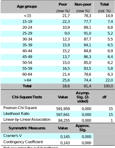
Table 1 – Poverty distribution by age Poor Non-poor Total Age groups
(row %) (row %) (col. %)
< 15 21,7 78,3 14,9 15-19 22,3 77,7 7,4 20-24 10,9 89,1 6,8 25-29 9,0 91,0 5,2 30-34 12,3 87,7 5,5 35-39 15,9 84,1 6,5 40-44 15,2 84,8 6,9 45-49 13,7 86,3 6,4 50-54 15,0 85,0 6,2 55-59 16,5 83,5 5,8 60-64 21,4 78,6 6,3 > 64 25,6 74,4 22,0 Total 18,6 81,4 100,0 Chi-Square Tests Value
Asymp. Sig. (2-sided) df Pearson Chi-Square 591,959 0,000 15 Likelihood Ratio 597,641 0,000 15 Linear-by-Linear Association 84,255 0,000 1
Symmetric Measures Value Approx. Sig.
Cramer's V 0,145 0,000
Contingency Coefficient 0,143 0,000 Not assuming the null hypothesis.
We observed that among the young people up to 14 years old the occurrence of poverty is 21,7%, contrasting the 18,6% in the general population, upholding other recent studies that arrive at similar conclusions, pointing out its weight among youth. The percentage of poor people in the nearest age group (15 to 19) is also higher than the global percentage, showing values that are significantly lower than the ones we find in the next age groups (20 to 59 years old).
The event of poverty is even more intense among people with ages higher than 65 years old, signifying 25,6% of the total elderly, being notoriously high within the great elderly (above 75 years old): 29,9%. Therefore, even if it‘s not possible to associate poverty to specific ages, the fact is that being between 31 and 64 years old lowers the probability of being poor in 21,7% (logit model). This probability is also inferior (-19,4%) among those who are between 15 and 30 years old (logit model).
Graph 2 – Poverty distribution by age
Poverty within age groups
5 10 15 20 25 30 < 15 15-19 20-24 25-29 30-34 35-39 40-44 45-49 50-54 55-59 60-64 > 64 Age groups Percentage Frequencies Global %
2.2. POVERTY AND GENDER
Being a woman increases the probability of being poor, even though the values between men and women do not show major differences: while among women poverty assumes 19,6% of the total, in the opposite sex only 17,5% were in a poverty condition.
However, the higher incidence of poverty among women is not homogeneously distributed along the age groups. The graph reading reveals that poverty prevails in young men and reverses in the senior age ranges.
2.3. POVERTY AND HOUSEHOLD DIMENSION
The analysis of poverty focused on the household dimension reveals the particular intensity of the phenomenon at both ends of the distribution. In fact, larger households as well as single or two person households are those which, proportionally, have more poverty situations.
As far as larger households are concerned, the incidence of poverty has a major effect on young people, as a result of their general overrepresentation in such situations, signifying the probable existence of women with high fertility rates.
Table 2 – Poverty distribution by household dimension Poor Non-poor Total Household dimension
(row %) (row %) (col. %)
1 37,3 62,7 6,4 2 22,3 77,7 21,8 3 12,4 87,6 22,4 4 13,0 87,0 25,7 5 19,6 80,4 12,8 6 19,2 80,8 5,8 7 27,9 72,1 2,6 8 17,2 82,8 0,8 9 40,9 59,1 0,7 10 50,0 50,0 0,4 11 33,3 66,7 0,4 12 50,0 50,0 0,1 13 66,7 33,3 0,1 Total 18,6 81,4 100,0 Chi-Square Tests Value
Asymp. Sig. (2-sided) df Pearson Chi-Square 1062,885 0,000 12 Likelihood Ratio 963,366 0,000 12 Linear-by-Linear Association 0,221 0,638 1
Symmetric Measures Value Approx.
Sig.
Cramer's V 0,194 0,000
Contingency Coefficient 0,190 0,000 Not assuming the null hypothesis.
Among single person households, over one third lives in a poverty situation, as shown in Table 2. Anyway, we can find even more meaningful values in households with 9 persons and over.
2.4. POVERTY AND EMPLOYMENT
To the extent that poverty relates to the individual condition or status facing employment, the most significant values are found among housewives (32,5%), followed by persons permanently incapacitated for work (29,3%), other inactive persons(24,1%), retired (22,0%) and students (21,2%).
Table 3 – Poverty distribution by job status
Poor
Non-poor Total Present job status
(row %) (row %) (col. %)
Employed 10,4 89,6 39,0
Employed (temporarily absent) 10,0 90,0 0,2
Unemployed 20,8 79,2 2,6
Compulsory armed forces service 11,9 88,1 0,1
Students 21,2 78,8 17,8
Housewives 32,5 67,5 10,3
Retired 22,0 78,0 21,6
Permanently incapacitated for work 29,3 70,7 1,8 Other inactive persons 24,1 75,9 6,5 Total 18,6 81,4 100,0 Chi-Square Tests Value
Asymp. Sig. (2-sided) df Pearson Chi-Square 1015,114 0,000 8 Likelihood Ratio 1029,301 0,000 8 Linear-by-Linear Association 736,523 0,000 1 Symmetric Measures Value Approx. Sig.
Cramer's V 0,189 0,000
Contingency Coefficient 0,186 0,000 Not assuming the null hypothesis.
2.5. POVERTY AND EDUCATION
There is an opposite relationship between poverty and education: poverty diminishes whenever the education level grows. This situation assumes real significance in Portugal, above all within those who achieve higher education levels.
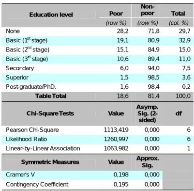
Table 4 – Poverty distribution by education level
Poor
Non-poor Total Education level
(row %) (row %) (col. %)
None 28,2 71,8 29,7 Basic (1st stage) 19,1 80,9 32,9 Basic (2nd stage) 15,1 84,9 15,0 Basic (3rd stage) 10,6 89,4 11,0 Secondary 6,0 94,0 7,5 Superior 1,5 98,5 3,6 Post-graduate/PhD. 1,6 98,4 0,2 Table Total 18,6 81,4 100,0 Chi-Square Tests Value
Asymp. Sig. (2-sided) df Pearson Chi-Square 1113,419 0,000 6 Likelihood Ratio 1260,997 0,000 6 Linear-by-Linear Association 1063,982 0,000 1
Symmetric Measures Value Approx. Sig.
Cramer's V 0,198 0,000
Contingency Coefficient 0,195 0,000 Not assuming the null hypothesis.
Poverty shows itself in a more meaningful way among the individuals who do not reach any level of education or merely hold the primary stage.
For those who achieve medium or higher levels of education, the event of poverty lowers in a very remarkable way.
Carrying out the secondary education level reduces the probability of being poor in 69,1% if compared to the remaining levels (Logit model). On the other hand, completing the higher level (superior) lets the equivalent probability fall by 92,3% (Logit model).
2.6. REGIONAL POVERTY
Poverty does not scatter in a homogenous manner alongside the national territory, displaying much more significant frequencies in the autonomous regions (25,5% in Açores and 23,8% in Madeira) than in the mainland (17,6% in Norte, 15,8% in Centro, 10,4% in Lisboa e Vale do Tejo, 13,6% in Alentejo and 14,6% in Algarve). The main highlights focus the region of Lisboa e Vale do Tejo, for the good reasons, and the autonomous regions, for the bad ones. If we regard the global mainland versus the islands as a whole, we draw one probability of being poor that is 42,5% smaller in the mainland (Logit model).
If we put the region of Lisboa e Vale do Tejo side by side with the islands (autonomous regions) e, we draw one probability of being poor that increases by 244% in Madeira and 253,6% in Açores (Logit model).
Another used breakdown was rural / semi-urban / urban area. The results depict a widespread of poverty in rural (25,5%) and semi-urban (20,0%) areas, in contrast with urban areas (11,5%), which underlines the belief of higher income in the cities. To live in a rural area increases the probability of being poor by 82,6%, if related to an urban area (Logit model).
We also analyse the occurrence of poverty as a function of the residence area (metropolitan or non-metropolitan). Coherently with the results previously found, the incidence of poverty reduces in the first (8,7%) and grows in the latter (20,3%).
3. POVERTY AMONG YOUNG PEOPLE
Throughout the depiction of data, we made sure that poverty was slightly higher among people under 15 years old if compared with the general phenomenon incidence. Within the 4214 young people (up to 14 years old), 913 we classified as poor (21,7%).
However, this outcome does not geographically distribute in an even way. In fact, at the same time as young poverty achieves 14,3% in the mainland, it doubles that score in the autonomous territories (islands), reaching 31,2%.
Table 5 – Poverty distribution within young people by household dimension Poor Non-poor Total
Household dimension
(row %) (row %) (col. %)
2 23,6 76,4 1,3 3 11,2 88,8 17,3 4 16,7 83,3 38,8 5 25,0 75,0 21,2 6 26,8 73,2 9,8 7 41,6 58,4 5,5 8 26,6 73,4 1,9 9 48,1 51,9 1,8 10 58,3 41,7 1,1 11 53,3 46,7 0,7 12 45,5 54,5 0,3 13 72,7 27,3 0,3 Total 21,7 78,3 100,0
The distribution of the young poor according to the rural/urban area breakdown shows 29,7% in the rural, 26,3% in the semi-urban and 14,7% in the urban areas.
Regarding young poverty as a function of the household dimension, we find the hardest occurrence of poverty in single parent households. Only in three or four person households we can find a lower percentage of young poor than the one observed in the total young population (21,7%).
In households with five or more persons the young poverty rate is always higher than 25%, reaching values like 58,3% (10 persons), 53,3% (11 persons) and 72,7% (13 persons). These values are expressive enough to point out the increasing frequency of poverty in large dimension households, in which the supposed mother’s fertility rates are much higher than the average rate.
Table 6 – Poverty incidence within young people by age and gender < 5 5 to 9 10 to 14
(col . %) (col . %) (col. %) Poor 21,3 21,5 23,5 Non-poor 78,7 78,5 76,5 Male Total 100,0 100,0 100,0 Poor 18,0 21,9 22,0 Non-poor 82,0 78,1 78,0 Gender Female Total 100,0 100,0 100,0
We must underline the fact that poverty within young people is proportionally more significant among the male gender, evidence that we won’t try to explain anyhow.
4. POVERTY AMONG ELDERLY PEOPLE
Resembling the situation of youth, but on a higher scale, poverty within elderly people is far superior to the one observed among the general population. As a matter of fact, the probability of being poor associated to the fact of being old is about 32,3% larger than in non-old persons. But who are, then, the poor elderly people?
Table 7 – Poverty incidence within elderly people by age and gender 65 to 69 70 to 74 > 74
(col . %) (col . %) (col. %) Poor 20,6 22,5 29,2 Non-poor 79,4 77,5 70,8 Male Total 100,0 100,0 100,0 Poor 23,3 23,2 30,4 Non-poor 76,7 76,8 69,6 Gender Female Total 100,0 100,0 100,0
Within the old persons in our sample – 57,9% women and 42,1% men – 25,6% are poor. The incident of poverty is almost always higher among women and is liable to increase within the grand elderly group (75 or more years old). In this age group poverty occurrence rises up to 29,9%.
Old uneducated persons are the most severely distressed by poverty: 31,7% of them are poor. Those proportions show a decreasing trend strictly opposite to the tendency revealed by the outcome scores as education level increases. Therefore, poverty prevalence in the succeeding education levels is as follows: basic education/first stage (18,6%), basic education/second stage (9,7%), basic education/third stage (5,8%) and secondary level (3,8%).
Within married old persons, poverty holds 22,7% of the whole elderly people and this percentage rises to 30,1% whenever unmarried (single, widower or divorced) are concerned.
In each hundred old individuals inhabiting rural areas, 35,6% are poor. That proportion lowers to 30,1% in semi-urban regions and to 14,3% in urban locations.
Some of the deeply unexplored data in this research relate to the weight, share and purpose of non-monetary income, being noteworthy in rural and semi-urban areas and significant the role it plays in weakening the harder impacts of monetary poverty.
With regard to territorial breakdown, 24,5% of the elderly residents in the mainland are poor, whilst this percentage rises up to 28,6% for those who inhabit the islands.
As to poverty within the elderly, related to household dimension (opposite to the outcomes of the young people’s scenario), the higher frequency of poor people occurs in single person households (old individuals living alone), as we can see in the following Table.
Table 8 – Poverty distribution within elderly people by household dimension Poor Non-poor Total
Household dimension
(row %) (row %) (col. %)
1 42,7 57,3 21,3 2 25,4 74,6 51,4 3 16,6 83,4 12,8 4 7,2 92,8 6,3 5 11,1 88,9 4,5 6 8,9 91,1 2,5 7 12,5 87,5 0,6 8 9,1 90,9 0,2 9 100,0 0,2 10 100,0 0,1 11 25,0 75,0 0,1 13 100,0 0,0 Total 25,6 74,4 100,0 CONCLUDING REMARKS
This study meant to describe poverty, as a complex and multidimensional phenomenon, trying to explain it in terms of the specific contribution of each different feature, monitoring one set of independent variables and the way they rela te to poverty.
Starting from an objective standpoint regarding poverty assessment – the monetary approach – we undertook the demonstration of that relationship, by:
a) Testing the likelihood of poverty being related to other variables;
b) Seizing it as a variable whose behaviour can be determined from significant predictors;
c) Searching for a rule that allows estimating the probability of being poor when specific features take place.
Using data taken from the latest Portuguese Household Budget Survey (IOF/2000), under the technical responsibility of the Portuguese national statistics office (INE), we started with the choice of a set of variables and built up the hypothesis that they might explain poverty.
In the first approach, the crosstabs chi-square tests computed for all dependent variables tabulated with poverty, showed very high significance values (always close to 0.000), indicating that there may be some relationship between each two pair of variables. However, the low values got in the test statistics indicated that the relationships between them were fairly weak.
The second approach – a multiple linear regression model – brought to light a much more obvious relationship between poverty and the set of selected independent variables, with particular evidence for educational level and residence area (urban, semi-urban and rural) as major predictors within de model. In fact, the first one displayed an explaining capacity three times greater than the second, all of
them getting highly significant coefficients (valid model fit in) and low multicollinearity values, indicating absence of intercorrelation between the model predictors. Furthermore, poverty is primarily associated to the female gender, young and elderly persons and people living in large households. With regard to the third approach, the logit analysis underlined the outcomes achieved through the multiple linear regression model, estimating the probability of being poor associated with each specific incident.
One last word about the shortcoming of approaching poverty from the viewpoint of relative monetary poverty, discarding non-monetary income, as a result. Procedures like these produce twisted outcomes, being suitable to find methodologies that would allow greater objectivity in such kind of research.
REFERENCES
BÚRIGO, Fábio Luiz, (2003), Pobreza, um conceito em transformação in Colóquio Internacional sobre Políticas Públicas, Pobreza e Exclusão Social”, Livro II, Ijuí, Unijuí; in
http://www.nesfi.ufsc.br/pobreza.pdf (22/03/2005);
COHEN-SOLAL, Marc, LOISY, Christian, (2001), Transferts sociaux et pauvreté en Europe, WP Études et Résultats, nº 104, Paris, DREES;
COSTA, Alfredo Bruto et al, (1998), Pobreza e Exclusão Social em Portugal, a Região de Lisboa e
vale do Tejo in DPP (1999), Prospectiva e Pla neamento, Volume V, Lisboa, Departamento de
Prospectiva e Planeamento, Ministério do Planeamento, pp 49-173;
PARENTE, Paulo (sd) Analysis of Poverty and Inequality in Portugal, using Quintile Regression in
http://www.ine.pt/prodserv/estudos/ficha.asp?x_estudoid=260 (20/01/2005)
RODRIGUES, Carlos Farinha, (1999), Repartição do Rendimento e Pobreza em Portugal (1994/95)
(uma comparação entre o Painel de Agregados Familiares e o Inquérito aos Orçamentos Familiares),
WP, Junho de 1999, Lisboa, CISEP/ISEG
SCHAUER, Thomas, RADERMACHER, Franz Josef, (2003), Igualdade e Diversidade na Era da
Informação, in www.terra-2000.org (20/01/2005)
SOARES, Regina, BAGO D’UVA, Teresa, (2002), Income, Inequality and Poverty, in
APPENDIX I – MULTIPLE LINEAR REGRESSION MODEL Model Summary Change Statistics Model Ra) R Square Adjusted R Square Std. Error of the Estimate R Square Change F Change df1 df2 Sig. F Change 1 0,459 0,211 0,211 732975,851 0,211 840,074 9,000 28268,000 0,000 a) Predictors: (Constant), Rural/Urban, Age group, Gender, Household dimension, Metropolitan/non-metropolitan, Mainland/Islands, Education level, Familial status, Present job status
ANOVA b)
Model Sum of Squares df Mean Square F Sig. a) 1 Regression 4061994802722760 9 451332755858084,000 840,074 0,000 Residual 15187084720492500 28268 537253598432,592
Total 19249079523215300 28277
a) Predictors: (Constant), Rural/Urban, Age group, Gender, Household dimension, Metropolitan/non-metropolitan, Mainland/Islands, Educat ion level, Familial status, Present job status
b) Dependent Variable: Disposable net monetary income Coefficients a) Unstandardized Coefficients Standardized Coefficients Model B Std. Error Beta t Sig. 1 (Constant) 372770,251 28987,856 12,860 0,000 Rural - Urban 129607,086 6004,569 0,124 21,585 0,000 Age group 3704,370 1310,117 0,021 2,828 0,005 Gender -33509,060 8873,145 -0,020 -3,776 0,000 Household dimension -37713,042 3069,993 -0,078 -12,284 0,000 Metropolitan/non-metropolitan 173318,744 13766,991 0,075 12,589 0,000 Mainland/Islands -55774,148 10034,021 -0,032 -5,559 0,000 Education level 232328,440 3561,471 0,397 65,234 0,000 Familial status 76362,759 10628,800 0,046 7,185 0,000 Present job status 5764,587 1820,492 0,020 3,166 0,002
Coefficients a) (continued)
Correlations Collinearity Statistics Model
Zero-order Partial Part Tolerance VIF
1 (Constant) Rural - Urban 0,217 0,127 0,114 0,848 1,179 Age group -0,023 0,017 0,015 0,528 1,894 Gender -0,023 -0,022 -0,020 0,967 1,034 Household dimension -0,069 -0,073 -0,065 0,694 1,441 Metropolitan/non-metropolitan 0,182 0,075 0,067 0,791 1,264 Mainland/Islands -0,099 -0,033 -0,029 0,838 1,193 Education level 0,411 0,362 0,345 0,753 1,328 Familial status 0,043 0,043 0,038 0,675 1,482 Present job status -0,161 0,019 0,017 0,721 1,386 a) Dependent Variable: Disposable net monetary income
Collinearity Diagnostics a)
Variance Proportions Model Dimension Eigenvalue Condition
Index (Constant) /Urban Rural/ Age group Gender Household dimension 1 1 7,039 1,000 0,000 0,002 0,002 0,002 0,002 2 1,023 2,623 0,000 0,001 0,000 0,000 0,001 3 0,611 3,395 0,000 0,002 0,025 0,000 0,009 4 0,456 3,928 0,000 0,000 0,005 0,005 0,003 5 0,379 4,309 0,001 0,004 0,012 0,004 0,019 6 0,191 6,076 0,000 0,000 0,093 0,004 0,356 7 0,111 7,969 0,003 0,063 0,120 0,116 0,017 8 0,091 8,780 0,000 0,523 0,014 0,475 0,001 9 0,080 9,393 0,001 0,271 0,462 0,225 0,261 10 0,019 19,401 0,994 0,136 0,266 0,169 0,331
Collinearity Diagnostics a) (continued)
Variance Proportions Model Dimension Eigenvalue Condition Index Metropolitan
/non- metropolitan Mainland/ /Islands Education level Familial status Present job status 1 1 7,039 1,000 0,003 0,004 0,003 0,004 0,003 2 1,023 2,623 0,425 0,174 0,001 0,001 0,001 3 0,611 3,395 0,162 0,174 0,005 0,236 0,001 4 0,456 3,928 0,028 0,139 0,041 0,124 0,256 5 0,379 4,309 0,261 0,410 0,152 0,064 0,023 6 0,191 6,076 0,000 0,085 0,181 0,119 0,009 7 0,111 7,969 0,005 0,007 0,411 0,245 0,615 8 0,091 8,780 0,079 0,004 0,008 0,006 0,004 9 0,080 9,393 0,030 0,002 0,038 0,200 0,008 10 0,019 19,401 0,007 0,000 0,160 0,000 0,078 a) Dependent Variable: Disposable net monetary income
APPENDIX II – LOGIT MODELS Number of obs = 28278 LR chi2(5) = 1413,22 Prob > chi2 = 0,0000 Pseudo R2 = 0,0520 Log likelihood = -12876,3 poverty Coef. Std. Error z P>|z| young adult -0,2155535 0,055315 -3,897 0,000 adult -0,2441352 0,045694 -5,343 0,000 elderly 0,2802575 0,048609 5,766 0,000 rural 0,6021887 0,034623 17,393 0,000 mainland -0,5530373 0,032261 -17,143 0,000 esc12 -1,174693 0,095406 -12,313 0,000 escsup -2,562949 0,252977 -10,131 0,000 _cons -1,122078 0,041542 -27,011 0,000 Number of obs = 28278 LR chi2(5) = 1375,46 Prob > chi2 = 0,0000 Pseudo R2 = 0,0506 Log likelihood = -12895,15 poverty Coef. Std. Error z P>|z| young 0,2351287 0,043734 5,376 0,000 elderly 0,5138432 0,036841 13,947 0,000 rural 0,6048178 0,034629 17,466 0,000 mainland -0,5564814 0,032194 -17,285 0,000 escob 1,459359 0,08827 16,533 0,000 _cons -2,815508 0,088125 -31,949 0,000 Number of obs = 28278 LR chi2(5) = 1384,34 Prob > chi2 = 0,0000 Pseudo R2 = 0,0510 Log likelihood = -12890,71 poverty Coef. Std. Error z P>|z| elderly 0,46332 0,035368 13,1 0,000 rural 0,5957026 0,03457 17,232 0,000 mainland -0,5638074 0,032128 -17,549 0,000 esc12 -1,218632 0,093676 -13,009 0,000 escsup -2,610724 0,252785 -10,328 0,000 _cons -1,295097 0,026909 -48,129 0,000