Comparison of 2D time-integrated, 3D time-integrated and 2D time-resolved portal dosimetry in detecting patient dose errors in external beam radiotherapy

UNIVERSIDADE DE LISBOA

FACULDADE DE CIÊNCIAS

DEPARTAMENTO DE FÍSICA

Comparison of 2D time-integrated, 3D time-integrated

and 2D time-resolved portal dosimetry in detecting

patient dose errors in external beam radiotherapy

Mestrado Integrado em Engenharia Biomédica e Biofísica

Perfil de Radiações em Diagnóstico e Terapia

Dissertação orientada por:

Prof. Dr. Frank Verhaegen, Head of Clinical Physics Research Department,

MAASTRO Clinic, Maastricht, The Netherlands

Prof. Dr. Luís Peralta, Departamento de Física, Faculdade de Ciências da

Universidade de Lisboa, Lisboa, Portugal

2016

“Trabalha como se tudo dependesse de ti; confia como se tudo dependesse de Deus.”

“Work as if everything depended on you; trust as if everything depended on God.”

i

Acknowledgements

First of all, I would like to express my deep gratitude to my external supervisor, Prof. Dr. Frank Verhaegen, who gave me the opportunity to work with him and a top research team at MAASTRO. His expertise and guidance were crucial to achieve my goals in this project. Thank you for being always available to share your knowledge with me with patience and kindness.

The second person I want to thank is my internal supervisor, Prof. Dr. Luís Peralta, who shared with me his passion for Dosimetry. I can say that it was your subject in my Master that made me follow this path of dosimetry in medical physics. Thank you for being always available to help me.

A special thanks goes out to my second external supervisor, Mark Podesta, who was so patient and kind to teach me even thought he was busy with his work, he always found time for me. Your expertise and guidance made me to become a better researcher. Thank you for always supporting and encouraging me to believe in my potential. It was a pleasure work, have fun and run with you! I would also like to express a special thanks to my third external supervisor, Lotte Schyns, who was always attentive to my work and available to help me no matter the circumstances. Thank you for your friendship and our coffee breaks!

I would also like to express my gratitude to the DGRT research group of MAASTRO. Our meetings were crucial to guide my project. I am also grateful for the help provided by the medical physicist Jonathan Martens during the CT acquisitions and the treatment planning insight provided by the medical physicist Chin Loon.

Special thanks goes out to the clinical physics research group for making me feel so welcome at MAASTRO. Thank you for always supporting me and show me the importance of friendship at work. It was amazing to share this experience almost every day with you. I will never forget our lunch times, coffee breaks and dinners out!

A ti, Verde, um sincero obrigado por partilhares esta experiência comigo. Embarcar nesta aventura não seria a mesma coisa sem ti! Obrigada pelo apoio incansável e por todos os momentos de diversão, não só nestes últimos sete meses, mas sobretudo ao longo destes fantásticos 5 anos de faculdade que criaram esta grande Amizade. Um obrigado especial também a ti, Robalo, pela Amizade, pelas palavras de carinho e encorajamento.

Um obrigado muito especial vai também para a Isabel e para o Gabriel. Ter-vos na MAASTRO foi uma sorte! Sorte não, pois acredito que nada acontece por acaso! Obrigada por todos os momentos divertidos (jantaradas, saídas, picnics, Carnaval…), por todos os conselhos, por todas as gargalhadas e por me terem feito sempre sentir tão bem acolhida. Obrigada pela vossa amizade! Obrigada também a ti, Sara, pela tua energia e alegria inesgotáveis que coloriam os nossos dias na MAASTRO! Um grande obrigado também a ti, Murillo, e a ti, Louise, pois apesar de não nos termos cruzado por muito tempo foi fantástico poder partilhar os últimos meses convosco.

ii

I want also to thank to my lovely housemates Fedi and Evi. It was amazing to meet you and to share these months with you. Thank you for all the moments we shared. I have never thought I could do friendships like these in the Netherlands.

Other special thank goes out to my athletics team in Maastricht - Hub team. Thank you for providing me the opportunity to join you doing something we love, running! It was amazing to train with you on the track even with snow! A special thank goes also to my amazing French friend Solène for all the trainings, dinners and funny moments we shared.

Obrigada também ao João Carreira e ao Tiago Leonardo, pela vossa amizade e por me fazerem experienciar fins-de-semana bem diferentes do habitual nestes sete meses onde dominava sempre a comida típica portuguesa. A ti, Geraldes, obrigada pela alegria que vieste trazer a Maastricht neste último mês e meio! Obrigada pela amizade, por todos os momentos de diversão e por todos os picnics onde não faltavam as sandes com barulho. A vocês, André, Litos, Guimarães e Zé Nuno, obrigada por me fazerem sentir em Lisboa mesmo estando na Holanda durante as nossas trips. Um grande obrigado também a vocês, Helena, Teresa, Marina, Sara, Rute, Gui, Bacalhau, Gustavo e restantes amigos tugas por me terem apoiado sempre não só ao longo destes sete meses, mas sobretudo ao longo destes 5 anos de faculdade!

Um obrigado muito especial à minha fantástica Equipa de Jovens de Nossa Senhora (incluindo o Samuel!) que mesmo estando em Portugal esteve sempre comigo no coração. Cada vez mais estou certa de que somos muito mais do que uma equipa o mês inteiro, o ano inteiro! Obrigada pela vossa amizade pura e verdadeira e por todas as reuniões via Skype!

Aos meus pais, Amélia e João Pedro, obrigada pelo vosso amor e apoio incondicional. Além de serem a razão de eu existir, tudo aquilo que sou é graças ao vosso exemplo e esta tese é por isso dedicada a vocês. Obrigada pelo esforço que sempre fizeram em prol da minha educação enquanto estudante em Lisboa, em Heidelberg e em Maastricht.

Ao meu irmão, à minha madrinha, à minha afilhada, aos meus avós e a toda a minha família um sincero obrigado pelo vosso amor e carinho que chegou sempre a Maastricht independentemente dos 2000 km de distância.

“Aqueles que passam por nós, não vão sós, não nos deixam sós. Deixam um pouco de si, levam um pouco de nós.” “Those who pass us by, do not go alone, do not leave us alone. They leave a little piece of themselves, take a little of us.”

Anthóine de Sant-Exuperie

iii

Abstract

In external photon beam radiotherapy, patient-related errors are common to occur during the treatment course of the patient. These errors, such as tumor regression or tumor shift, may result in discrepancies between the planned and the actually delivered dose distribution to the patient. In this way, it is vital to perform dose verification during the treatment course of the patient to detect these errors and ensure treatment quality. The Electronic Portal Imaging Device (EPID) has been used as a tool for performing both pre-treatment and in-treatment dose verification. Since the introduction of more complex beam delivering techniques, especially Volumetric Modulated Arc Therapy (VMAT), more complex dose verification methods based in EPID dosimetry have also been introduced such as 2D time-integrated portal dosimetry, 3D time-integrated portal dosimetry and, more recently, 2D time-resolved portal dosimetry.

The main goal of this project was to compare the performance of 2D integrated, 3D time-integrated and 2D time-resolved portal dosimetry in detecting dose discrepancies caused by simulated errors related to the patient’s anatomy.

Multiple tumor shifts, tumor regressions and pleural effusion (excess fluid that accumulates in the pleural cavity) levels inside the lung were simulated in the planning CT-scan of six lung cancer patients treated with VMAT at MAASTRO clinic. Portal dose images were calculated in the original and manipulated planning-CT scans with the three portal dosimetry methods. For dose comparison 2D time-integrated, 2D-time resolved and 3D time-integrated gamma analyses were performed for each geometrical change and each patient employing five different gamma criteria. As main results, 3D time-integrated portal dosimetry demonstrated the highest performance (AUC = 0.85) in detecting tumor shifts and 2D time-resolved portal dosimetry revealed the highest performance in detecting tumor regressions (AUC = 0.93) and pleural effusion. A correlation between D95% changes

in the DVHs and gamma fail rates was found at individual patient level but not at the patient cohort level.

A phantom experiment was done to replicate the tumor shifts simulated in the patients. A set of simulations and measurements were performed following the same protocol. The dynamic thorax phantom was irradiated with VMAT for each tumor shift applied. The dose to the tumor was determined with film dosimetry and EPID images were collected during each irradiation. The results revealed that the phantom simulations and measurements follow the same behavior. The 2D time-resolved portal dosimetry showed to be able to detect more dose discrepancies caused by the tumor shifts than 2D time-integrated portal dosimetry.

As main conclusion, 2D resolved portal dosimetry was superior in general to 2D and 3D time-integrated portal dosimetry in detecting dose discrepancies caused by geometrical changes within the patients and the phantom. Time-resolved portal dosimetry is able to highlight discrepancies that are not shown when only the integrated portal dose images are compared.

iv

Resumo

Em radioterapia externa com feixes de fotões é essencial que a distribuição de dose planeada seja entregue ao paciente com elevada precisão de modo a garantir a qualidade do tratamento. No entanto, existem certos tipos de erros que podem ocorrer durante as várias fracções de tratamento do paciente e prejudicar assim a qualidade do tratamento. Esses erros podem estar relacionados com o linac (acelerador linear) - posições incorrectas dos colimadores multi-folhas - ou com o paciente - erros de posicionamento do paciente ou alterações geométricas na anatomia do paciente. Os erros de posicionamento do paciente, como é o caso da translação ou rotação do paciente, podem fazer com que o feixe de radiação não atinja o tumor acabando por prejudicar o tecido saudável que se encontra à sua volta. No que diz respeito às alterações geométricas, as mais frequentes no decorrer do tratamento de radioterapia em pacientes com cancro no pulmão são o desvio do tumor, a regressão do tumor e a efusão pleural (excesso de fluido que se acumula na cavidade pleural). Estas alterações geométricas podem resultar numa discrepância entre a distribuição de dose planeada e a distribuição de dose que é realmente entregue ao paciente prejudicando assim a qualidade do tratamento. Deste modo, torna-se fundamental verificar a entrega da distribuição de dose quer antes quer durante o decorrer do tratamento do paciente de forma a detectar estes tipos de erros e garantir assim a qualidade do tratamento.

Outro factor que também tem contribuído para uma maior exigência das práticas de verificação de dose durante o tratamento do paciente é o aparecimento de novas técnicas de radioterapia externa mais complexas que envolvem mais graus de liberdade, como é o caso da técnica de VMAT (terapia de arco volumétrico). O aumento da complexidade destas técnicas aumenta também a complexidade do tratamento e leva por isso a uma maior exigência na validação e controlo de qualidade (QA) do tratamento.

Existem várias ferramentas de verificação de dose utilizadas em prática clínica para QA do tratamento e para detecção de discrepâncias de dose, como é o caso das câmaras de ionização, dos EPIDs (electronic portal imaging devices), dos filmes radiocrómicos, dos géis de polímeros ou outros detectores. O EPID tem sido o detector mais utilizado actualmente para a verificação de dose antes e durante o tratamento de radioterapia. Este detector obtém a distribuição de dose medida que depois é comparada com a distribuição de dose planeada (prevista). A análise gama é o método quantitativo mais utilizado para comparação de distribuições de dose. Este método utiliza em simultâneo dois critérios, a percentagem de diferença de dose (DD) e a distância de concordância (DTA), para o cálculo do índice gama pixel por pixel ou voxel por voxel. Ao aplicar um critério de aceitação (ex.: 3%, 3 mm), as discrepâncias entre as distribuições de dose de extensão geométrica e magnitude variável podem ser identificadas.

Esta tese centra-se em dosimetria portal de transmissão em que o paciente se encontra entre o feixe de radiação e o EPID que mede a distribuição de dose entregue ao paciente. O aparecimento de novas técnicas de radiação mais complexas, como IMRT (radioterapia de intensidade modulada) e VMAT também tem levado ao desenvolvimento de novos métodos de verificação de dose com base em EPID. O método de 2D time-resolved portal dosimetry foi introduzido recentemente para a

v

técnica VMAT. Este método diferencia-se pelo facto de o EPID ler a distribuição de dose para cada segmento (duração compreendida entre dois pontos de controlo consecutivos) do VMAT em vez de ler apenas a distribuição de dose cumulativa (time-integrated portal dosimetry).

O principal objectivo desta tese é a comparação do desempenho dos métodos 2D time-integrated, 3D time-integrated e 2D time-resolved portal dosimetry na detecção de discrepâncias de dose em pacientes com cancro no pulmão causadas pela simulação de alterações geométricas na anatomia do paciente.

Para tal foram simulados múltiplos desvios do tumor, múltiplas regressões do tumor e múltiplos níveis de efusão pleural (fluido que se acumula na cavidade pleural) em cada CT (Tomografia Computorizada) de planeamento de seis pacientes com cancro no pulmão que foram tratados com VMAT na MAASTRO Clinic. Também se procedeu ao cálculo de imagens de dose portal no CT de planeamento original e em cada CT manipulado (CT com a alteração geométrica já aplicada) recorrendo aos três métodos de dosimetria portal já referidos. De forma a comparar a dose planeada com a dose medida, foram feitas 2D time-integrated, 2D time resolved e 3D time-integrated

gamma analyses para cada alteração geométrica simulada e para cada paciente utilizando cinco

critérios gama diferentes.

Posteriormente, foi investigado o desempenho de cada um destes métodos através da construção de curvas ROC (Receiver Operating Characteristic) e da determinação dos valores da área sob a curva (AUC). Como principais resultados, 3D time-integrated portal dosimetry foi o método que demonstrou o melhor desempenho (AUC = 0.85) na detecção de desvios do tumor e 2D

time-resolved portal dosimetry foi o método que revelou o melhor desempenho na detecção de

regressões do tumor (AUC = 0.93) e de efusão pleural.

Além disso também foi estudada a correlação entre a variação da métrica D95% do DVH (Dose Volume Histogram) calculado para cada paciente e as gamma fail rates obtidas para cada paciente e

para cada tipo de alteração geométrica com cada método de dosimetria portal já referido. Esta correlação foi estudada tendo em consideração apenas um paciente, e tendo em consideração os seis pacientes como um grupo. Como resultado verificou-se que existe correlação a nível individual, mas não a nível colectivo. O facto de haver correlação a nível individual é bastante importante pois significa que no futuro será possível obter uma curva de regressão para cada simulação de um paciente e prever qual será a variação da métrica D95% a partir das gamma fail rates medidas e

decidir assim quando adaptar o plano de tratamento do paciente em causa.

Para além das simulações nos pacientes, também foi realizada uma experiência com um fantoma representativo do tórax humano (CIRS dynamic thorax phantom) com o intuito de replicar os desvios do tumor simulados nos pacientes. Foi feito um conjunto de simulações e medições experimentais seguindo o mesmo protocolo. No que diz respeito às medições experimentais, foi construído um mini-fantoma representativo do tumor (dois cilindros de PMMA -

polymethylmethacrylate) com tecido pulmonar à volta (esponja) de forma a possibilitar a colocação

de um filme radiocrómico entre os dois cilindros de PMMA. Nesta experiência foi feita uma irradiação com VMAT para cada desvio do tumor (mini-fantoma) aplicado no dynamic thorax

phantom e a dose recebida no tumor foi medida em cada irradiação através de dosimetria com filme

radiocrómico. Além disso, também foram adquiridas imagens portais do EPID durante cada irradiação. Os resultados deste estudo revelaram que as simulações e medições com o fantoma

vi

seguem o mesmo comportamento. O método 2D time-resolved portal dosimetry demonstrou ter capacidade para detectar mais discrepâncias de dose causadas por desvios do tumor do que 2D

time-integrated portal dosimetry.

Como principal conclusão, 2D time-resolved portal dosimetry demonstrou ser o melhor método na generalidade para detectar discrepâncias de dose causadas por alterações geométricas da anatomia dos pacientes e no fantoma. Este novo método de dosimetria portal foi capaz de identificar discrepâncias de dose que não são reveladas quando se comparam apenas integrated portal dose

images.

vii

Contents

Acknowledgements ... i Abstract ...iii Resumo ... iv Contents ... vii List of Figures ... ix

List of Tables ... xiii

List of Abbreviations ... xiv

Preface ... 1 Introduction ... 2 1 Background ... 3 2 2.1 Cancer ... 3 2.1.1 Treatment options ... 3 2.2 Radiotherapy ... 3

2.2.1 External Mega Voltage Photon Beam Radiotherapy ... 4

2.2.2 Radiotherapy workflow ... 5 2.2.2.1 Preparation ... 5 2.2.2.2 Treatment Delivery ... 6 2.2.2.2.1 IMRT ... 7 2.2.2.2.2 VMAT... 7 2.2.2.3 Treatment verification ... 8 2.2.2.3.1 Position verification ... 8

2.2.2.3.2 Dose verification (portal dosimetry) ... 8

2.2.2.3.2.1 Gamma evaluation method ... 8

2.2.2.4 Adaptive radiotherapy ... 10

2.3 State-of-the-art of EPID dosimetry ... 11

2.3.1 a-Si EPID ... 11

2.3.2 Methods based on EPID dosimetry ... 12

2.3.2.1 Transit portal dosimetry ... 12

2.3.2.2 2D Transit portal dosimetry... 13

2.3.2.3 3D (in vivo) portal dosimetry ... 13

2.3.2.4 Time-integrated and time-resolved portal dosimetry for VMAT ... 14

2.3.2.4.1 Clinical approaches ... 15

2.3.2.4.1.1 2D Time-integrated portal dosimetry ... 15

2.3.2.4.1.2 3D Time-integrated portal dosimetry (3D in vivo dosimetry) ... 15

viii

Materials & Methods ... 18

3 3.1 Materials ... 18

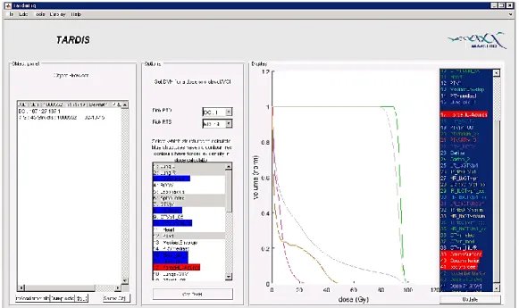
3.1.1 Clinical equipment and software ... 18

3.1.2 Research software ... 18 3.2 Methods ... 19 3.2.1 Patient simulations ... 19 3.2.1.1 Tumor shift ... 19 3.2.1.2 Tumor regression ... 21 3.2.1.3 Pleural effusion ... 22 3.2.2 Dose evaluation ... 23

3.2.3 Correlation analysis between gamma results and differences in D95% metric ... 25

3.2.4 Sensitivity and specificity of the gamma analysis ... 25

3.2.5 Phantom simulations and measurements ... 26

3.2.5.1 Phantom characteristics ... 26

3.2.5.2 Phantom treatment plan ... 27

3.2.5.3 Phantom simulations ... 29

3.2.5.4 Phantom measurements ... 29

3.2.5.5 Comparison between phantom simulations and measurements ... 30

3.2.6 Supplementary study ... 30

4 Results ... 31

4.1 Patient simulations – a single patient ... 31

4.1.1 Tumor shift... 31

4.1.2 Tumor regression ... 34

4.1.3 Pleural effusion ... 37

4.2 Correlation analysis ... 43

4.2.1 Correlation analysis in a single patient ... 43

4.2.2 Correlation analysis in six patients ... 45

4.3 Sensitivity and specificity of the gamma analysis... 46

4.3.1 Tumor shift... 46

4.3.2 Tumor regression ... 49

4.4 Phantom simulations and measurements ... 52

4.4.1 Time-integrated and time-resolved gamma analyses ... 53

4.5 Supplementary study... 57

4.5.1 Correlation between gamma failure and survival days ... 57

4.5.2 Correlation between gamma failure and tumor volume ... 58

5 Discussion ... 59

6 Conclusion and Future Work ... 61

Appendix ... 62

ix

List of Figures

Figure 2.1 - TrueBeam Varian High Energy linac equipped with (1) an electronic portal imaging

device (EPID) which acquires MV images of the treatment beam and (2) a kilo Volt (kV) imaging system [15]. ... 4

Figure 2.2 - Schematic overview of the external photon beam radiotherapy workflow. The feedback

loop which involves treatment adaptation is also called adaptive radiotherapy. ... 5

Figure 2.3 - Representation of cumulative DVHs. The ideal cumulative DVHs are represented on the

right (b) for a target structure (prostate) and a critical structure (bladder) [17]... 6

Figure 2.4 - Comparison between an IMRT (left) and a VMAT (right) plan. The VMAT plan was

obtained with the RapidArc system commercialized by Varian Medical Systems. The VMAT plan shows a more conformed dose distribution [21]. ... 7

Figure 2.5 - Example of a time-integrated gamma analysis. The hot spot shown in red represents an

over-dosage whereas the cold spot shown in blue represents an under-dosage. ... 9

Figure 2.6 - aSi 1000 EPID from Varian Medical Systems. ... 11 Figure 2.7 - Representation of the different arrangements for EPID dosimetry, each one with the

possibility to verify a dose distribution at the EPID level or inside the patient or phantom. Adapted from [6]. ... 12

Figure 2.8 - Schematic representation of the several steps involved in the model used for 3D in vivo

dosimetry developed by van Elmpt. In a first step the 2D open-field portal dose images acquired by the EPID from all beam directions are converted to energy fluence. This energy fluence is then back-projected to level of the linac. Based on this new energy fluence distribution, a forward Monte Carlo 3D dose calculation is done inside the patient’s planning CT or CBCT scan. As a result, a reconstructed 3D dose distribution in the planning CT or CBCT scan is obtained. ... 14

Figure 2.9 - Workflow of the 3D portal dose measurement acquisition and extraction of dose

metrics from the DVH and γ evaluations. On the left side a typical treatment planning process is depicted. On the right side the treatment process is depicted, the acquisition of the PDM. Adapted from [29]... 16

Figure 2.10 - Schematic overview of 2D time-resolved portal dosimetry (time-resolved transit

planar dosimetry) for VMAT. The measured transit planar portal dose images per CP during treatment are compared to the predicted transit portal dose images per CP. A time-resolved gamma evaluation is used for dose comparison. The gamma evaluation results can be expressed by a gamma map or by a polar plot as function of the gantry angle where the red region represents an over-dosage and the blue region represents an under-dosage. Adapted from [45]... 17

x

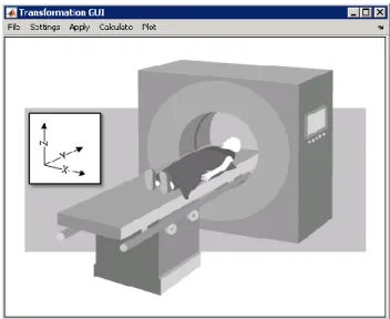
Figure 3.2 - Snapshot of the Transformation GUI software. The representation of the X, Y and Z axis

was used as reference for this thesis. ... 20

Figure 3.3 - Example of simulated tumor shifts of different magnitudes along the positive direction

of Y axis. The blue contour represents the original PTV and the red contour represents the GTV (tumor structure). Top left: original CT (without tumor shift). Top center: 0.5 cm tumor shift. Top right: 1.0 cm tumor shift. Bottom left: 1.5 cm tumor shift. Bottom center: 2.0 cm tumor shift. Bottom right: 2.5 cm tumor shift. ... 21

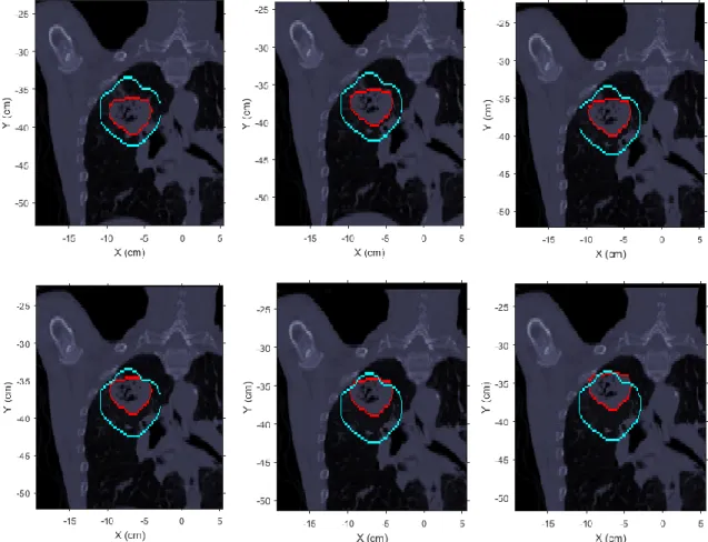
Figure 3.4 - Example of simulated tumor regressions of different magnitudes. The blue contour

represents the original PTV and the red contour represents to the GTV (tumor structure). Top left: original CT (without tumor regression). Top center: 10% of tumor regression. Top right: 30% of tumor regression. Bottom left: 50% of tumor regression. Bottom center: 70% of tumor regression. Bottom right: 90% of tumor regression... 22

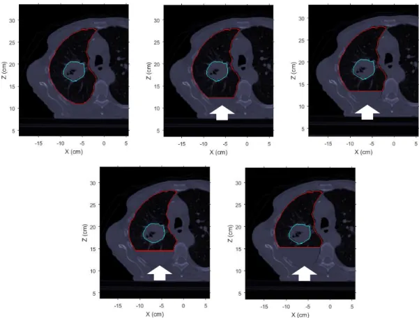
Figure 3.5 - Example of simulated pleural effusion of different magnitudes inside the left lung. The

blue contour represents the GTV (tumor structure) and the red contour represents the right lung which contains the tumor. Top left: original CT (without pleural effusion). Top center: 1 cm of fluid level. Top right: 2 cm of fluid level. Bottom left: 3 cm of fluid level. Bottom right: 4 cm of fluid level. ... 23

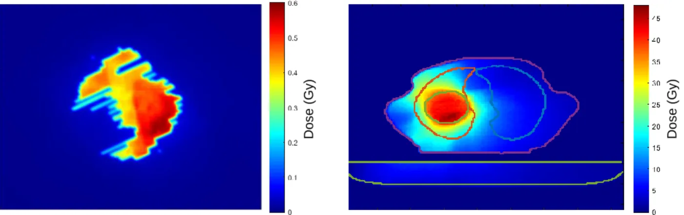
Figure 3.6 - Example of 2D and 3D dose distributions. Left: portal dose image at the EPID level. The

shape of the dose distribution is caused by the position of the MLCs. Right: portal dose image reconstructed in 3D at the patient level. The couch is represented in the bottom (light green contour) and the body structure is represented in the center (XZ plane). The tumor (green contour) is inside the left lung (red contour). ... 24

Figure 3.7 - CIRS Dynamic Thorax Phantom... 26 Figure 3.8 - Representation of the two parts of the insert composed by sponge and PMMA without

the film piece (left) and with the film piece (right). ... 27

Figure 3.9 - Representation of the lung equivalent rod of the phantom with the air gap on the top to

introduce the whole insert. ... 27

Figure 3.10 - Axial slice of the CT image of the phantom with the new tumor model insert inside the

left lung. ... 28

Figure 3.11 - Representation of the treatment plan of the phantom in ARIA research software

(Varian Medical Systems). ... 28

Figure 3.12 - Setup of the phantom measurements. The phantom is positioned at the isocenter of

the linac and the on-board EPID is under the couch. ... 29

Figure 4.1 - DVH curves for the original GTV and each shifted GTV. The red line represents the DVH

of the original GTV and the other colors represent the DVH of each shifted GTV. ... 32

Figure 4.2 - Difference in D95% metric of the GTV DVH as function of the GTV shift along the Y axis.

... 32

Figure 4.3 - Gamma fail rates (percentage of failing pixels) for the tumor shift simulations obtained

with 2D time-integrated portal dosimetry. ... 33

Figure 4.4 - Gamma fail rates (percentage of failing pixels) for the tumor shift simulations obtained

xi

Figure 4.5 - Gamma fail rates (percentage of failing voxels) for the tumor shift simulations obtained

with 3D time-integrated portal dosimetry. ... 34

Figure 4.6 - DVH curves for the original GTV and each transformed GTV. The different color lines

represent different tumor regressions. The DVH for the original GTV is represented in red. ... 35

Figure 4.7 - Difference in D95% metric of the GTV DVH as function of the GTV regression. ... 35

Figure 4.8 - Gamma fail rates (percentage of failing pixels) obtained with 2D time-integrated portal

dosimetry as function of the new tumor volume and the gamma criteria. ... 36

Figure 4.9 - Gamma fail rates (percentage of failing pixels) obtained with 2D time-resolved portal

dosimetry as function of the new tumor volume and the gamma criterion. ... 36

Figure 4.10 - Gamma fail rates (percentage of failing voxels) obtained with 3D time-integrated

portal dosimetry as function of the new tumor volume and the gamma criteria. ... 37

Figure 4.11 - DVH curves for the GTV after the simulation of different levels of pleural effusion in

the lung which contains the tumor. The red line represents the original GTV without the presence of fluid volume in the lung. ... 38

Figure 4.12 - Difference in D95% metric of the GTV DVH as function of the level of pleural effusion in

the lung which contains the tumor. ... 38

Figure 4.13 - Gamma fail rates (percentage of failing pixels) obtained with 2D time-integrated

portal dosimetry as function of the fluid volume in the lung which contains the tumor and the gamma criteria. ... 39

Figure 4.14 - Gamma fail rates (percentage of failing pixels) obtained with 2D time-resolved portal

dosimetry as function of the fluid volume in the lung which contains the tumor and the gamma criteria. ... 39

Figure 4.15 - Gamma fail rates (percentage of failing voxels) obtained with 3D time-integrated

portal dosimetry as function of the fluid volume in the lung which contains the tumor and the gamma criteria. ... 40

Figure 4.16 - Correlation between the difference in D95% and the gamma fail rate obtained with 2D

time-integrated (left), 2D time-resolved (middle) and 3D time-integrated (right) gamma analyses resultant from the tumor shifts simulations in one patient case. ... 43

Figure 4.17 - Correlation between the difference in D95% and the gamma fail rate obtained with 2D

time-integrated (left), 2D time-resolved (middle) and 3D time-integrated (right) gamma analyses resultant from tumor regression simulations for one patient case. .. 44

Figure 4.18 - Correlation between the difference in D95% and the gamma fail rate obtained with 2D

time-integrated (left), 2D time-resolved (middle) and 3D time-integrated (right) gamma analyses resultant from pleural effusion simulations for one patient case. ... 44

Figure 4.19 - Correlation between the difference in D95% and the gamma fail rate obtained with 2D

time-integrated (left), 2D time-resolved (middle) and 3D time-integrated (right) gamma analyses resultant from the tumor shifts simulations in six patients. ... 45

xii

Figure 4.20 - Correlation between the difference in D95% and the gamma fail rate obtained with 2D

time-integrated (left), 2D time-resolved (middle) and 3D time-integrated (right) gamma analyses resultant from the tumor shrinkage simulations in six patients. ... 45

Figure 4.21 - Correlation between the difference in D95% and the gamma fail rate obtained with 2D

time-integrated (left), 2D time-resolved (middle) and 3D time-integrated (right) gamma analyses resultant from the pleural effusion simulations in six patients. ... 46

Figure 4.22 - ROC curves resultant from the tumor shift simulations for 2D time-integrated and 2D

time-resolved gamma analyses and for all the five gamma criteria used. ... 47

Figure 4.23 - ROC curves resultant from the tumor shift simulations for 3D time-integrated gamma

analysis and for all the five gamma criteria used. ... 47

Figure 4.24 - AUC values for the ROC curves generated from the tumor shift simulations for 2D

time-integrated, 2D time-resolved and 3D time-integrated gamma analyses. ... 48

Figure 4.25 - ROC curves resultant from the tumor regression simulations for 2D time-integrated

and 2D time-resolved gamma analyses and for all the five gamma criteria used. ... 49

Figure 4.26 - ROC curves resultant from the tumor regression simulations for 3D time-integrated

gamma analysis and for all the five gamma criteria used. ... 50

Figure 4.27 - AUC values for the ROC curves generated from the tumor regression simulations for

2D time-integrated, 2D time-resolved and 3D time-integrated gamma analyses. ... 51

Figure 4.28 - CT image and respective 3D dose distribution correspondent to the original tumor

position (top left) and each tumor shift along the negative direction of Y axis. ... 52

Figure 4.29 - Mean dose inside the region of interest of the film for each tumor shift along the

negative direction of Y axis. The blue and red curves represent the phantom simulations and measurements, respectively. ... 53

Figure 4.30 - Correlation between the days of survival and the absolute gamma fail area per beam

inside the field mask obtained with 2D time-integrated gamma analysis (left) and between the days of survival and the gamma fail area per segment inside the field mask obtained with 2D time-resolved gamma analysis (right) for [4%, 4 mm] gamma criterion. ... 57

Figure 4.31 - Correlation between the tumor volume and the absolute gamma fail area per beam

inside the radiation field mask obtained with 2D time-integrated gamma analysis (left) and between the days of survival and the gamma fail area per segment inside the radiation field mask obtained with 2D time-resolved gamma analysis (right) for [1%, 1 mm] gamma criterion. ... 58

Figure A.1 - Representation of 10 cm of water equivalent slab phantoms with a film piece

positioned at the top at the isocenter of the linac.. ... 62

Figure A.2 - The correction factor hw,m as a function of depth for the field size 10 cm x 10 cm [58]...

... 63

xiii

List of Tables

Table 4.1 - 2D Time-integrated and time-resolved gamma analyses (3%, 3 mm) for the simulated

levels of pleural effusion in the lung which contains the tumor. ... 41

Table 4.2 - Optimal thresholds (%) obtained for 2D time-integrated, 2D time-resolved (% of failure

inside the field mask) and 3D time-integrated (% of failure inside the GTV) gamma analysis corresponding to each gamma criterion for the tumor shift simulations. ... 48

Table 4.3 - Optimal thresholds (%) obtained for 2D time-integrated, 2D time-resolved (% of failure

inside the field mask) and 3D time-integrated (% of failure inside the GTV) gamma analysis correspondent to each gamma criterion for the tumor regression simulations. ... 50

Table 4.4 - Time-integrated and time-resolved gamma analyses (3%, 3 mm) for each tumor shift

inside the left lung of the phantom. ... 54

Table A.1 - Machine outputs applied for each film irradiation and corresponding dose values. ... 63 Table A.2 - Fit parameters of the calibration curve for red channel. ... 65

xiv

List of Abbreviations

ART Adaptive Radiation Therapy

AUC Area Under the Curve

CBCT Cone Beam Computed Tomography

CP Control Point

CT Computed Tomography

CTV Clinical Target Volume (= GTV + margin for subclinical disease)

DGRT Dose Guided Radiation Therapy

DICOM Digital Imaging and Communication in Medicine

DNA Deoxyribonucleic acid

DPI Dots Per inch

DTA Distance To Agreement

DVH Dose Volume Histogram

EBRT External Beam Radiation Therapy

EPID Electronic Portal Imaging Device

GTV Gross Tumor Volume

HU Hounsfield Unit

IGRT Image Guided Radiation Therapy

IMRT Intensity Modulated Radiation Therapy

linac linear accelerator

MAASTRO Maastricht Radiation Oncology

MLC Multi Leaf Collimator

MRI Magnetic Resonance Imaging

MU Monitor Unit

MUMC+ University Hospital Maastricht

NSCLC Non-Small Cell Lung Cancer

OAR Organs At Risk

OD Optical Density

PD Percentage Difference

PDD Percentage Depth Dose

xv

PMMA Polymethylmethacrylate

PTV Planning Target Volume (= CTV + margin for geometrical uncertainties)

PV Pixel Value

QA Quality Assurance

ROC Receiver Operating Characteristic

RT Radiation Therapy

TIFF Tagged Image File Format

TPS Treatment Planning System

TTA Time To Agreement

VMAT Volumetric Modulated Arc Therapy

WHO World Health Organization

1

Preface

This project was carried out at the Clinical Physics Research department of MAASTRO (Maastricht Radiation Oncology) Clinic in Maastricht, The Netherlands. MAASTRO Clinic was founded in 1977 and is a radiotherapy institute that provides state-of-the-art radiation therapy for various types of cancer to approximately 4000 cancer patients each year in Limburg, south-east region of the Netherlands.

MAASTRO Clinic currently has six TrueBeam linear accelarators (linacs) from Varian, all equipped with EPID (electronic portal imaging device) and with CBCT (Cone Beam Computed Tomography). It also has 2 CT scanners and was the first center with a CT-PET scanner dedicated for radiotherapy, which now includes the possibility to acquire dynamic PET (Positron Emission Tomography) scans and 4D-CT-PET in lung cancer patients.

MAASTRO works closely with the radiotherapy department of the University Hospital Maastricht (MUMC+) and are developing together the South-East Netherlands Proton Therapy Center (ZON-PTC).

Currently, the Physics Research group has five research groups: dose-guided radiotherapy (DGRT), brachytherapy, proton therapy, advanced imaging and small animal radiotherapy. The project presented in this thesis was involved on the DGRT research group which focuses on performing accurate verification of the dose delivered to the patient.

The supervisor of this project was Prof. Dr. Frank Verhaegen, head of Clinical Physics Research department at MAASTRO, and the internal supervisor was Prof. Dr. Luís Peralta from the Physics department at Faculty of Sciences, University of Lisbon, Portugal. This project also had as associated supervisors Mark Podesta and Lotte Schyns, PhD students from the Clinical Physics Research department at MAASTRO.

2

Introduction

1

The development of more complex beam delivery techniques in external photon beam radiotherapy (EBRT), such as Intensity Modulated Radiotherapy (IMRT) and Volumetric Modulated Arc Therapy (VMAT), has increased the need for accurate verification of the dose delivery during patient treatment to ensure treatment quality.

Since VMAT uses many degrees of freedom during dose delivery, quality assurance (QA) is more difficult to perform for VMAT than for the conventional static radiation delivery techniques. Several verification devices specialized for arc trajectories have been used for performing VMAT QA, namely ArcCHECK (Sun Nuclear Corporation, Melbourne, FL), MatriXX (IBA, Schwarzenbruck, Germany) and Ocatvius (PTW, Freiburg, Germany) [1]. Apart from these devices, Electronic Portal Imaging Devices (EPIDs) have been used as an accurate tool for performing both pre-treatment and in-treatment dose delivery verification including time-integrated portal dosimetry and more recently, time-resolved portal dosimetry [2-4].

Pre-treatment QA is able to detect dose delivery changes caused by problems related to the linac, such as errors in the beam delivery. However, dose delivery deviations caused by changes in patient anatomy can only be detected on the day of the treatment or during treatment. This project has focused on dose delivery errors due to geometrical changes in patient anatomy that can frequently and rapidly occur over the course of fractionated EBRT. Tumor regression, tumor shift and pleural effusion in the lungs are examples of such geometrical changes [5]. If not detected, these changes may cause the actually delivered dose to deviate from the planned dose, thereby damaging the surrounding healthy tissues instead of the tumor.

In order to identify these dose delivery deviations in VMAT there are several EPID-based methods suitable for performing dose delivery verification. This project will focus on transit portal dosimetry in which EPIDs are used to obtain measured dose distributions behind the patient. Transit portal dosimetry is able to detect errors related to the beam delivery system itself and errors related to the patient [6]. Within transit portal dosimetry, 2D and 3D time-integrated portal dosimetry are currently employed in some radiotherapy centers [6-9]. Time-resolved portal dosimetry has been recently introduced for VMAT (Podesta et al. 2014 a) and has offered added value in assessing dynamic treatments. Instead of reading out the cumulative dose distribution to the EPID (time-integrated portal dosimetry), the dose distribution for each VMAT (time) segment is read out separately (time-resolved portal dosimetry) [2].

The main goal of this project is to compare the performance of three different transit portal dosimetry methods in detecting dose delivery deviations caused by patient anatomical changes: 2D time-integrated portal dosimetry, 3D time-integrated portal dosimetry (3D in vivo dosimetry) and 2D time-resolved portal dosimetry.

3

Background

2

2.1 Cancer

Cancer is characterized by the uncontrolled growth and spread of abnormal cells. If this spread is not controlled, it can result in serious illness and death. Cancer has become one of the greatest public health problems worldwide being one of the leading causes of morbidity and mortality. In 2008 there were 3.2 million new cases of cancer and 1.7 million deaths from cancer in Europe [10]. In the United States the estimated number of new cancer cases projected for 2015 was 1,658,370 and it was expected that about 589,430 Americans would die from cancer [11]. According to the World Health Organization (WHO), in twenty years from now the number of new cases of cancer will increase by 70% to more than 22 million cases [12].

2.1.1 Treatment options

Nowadays there are three main modalities for treating cancer: surgery, chemotherapy and radiotherapy. Surgery is usually done when the tumor is accessible or when organ preservation is not an essential requirement. Chemotherapy uses systemic agents (drugs) to kill the abnormal cells which are dividing rapidly. In this way, in several cases chemotherapy is used together with surgery and radiation therapy. Radiation therapy (radiotherapy) uses ionizing radiation to destroy the cancer cells. The most common types of ionizing radiation used are electrons, photons, protons and heavy ions (e.g.: carbon).

2.2 Radiotherapy

Radiotherapy is one of the main modalities for treating cancer next to surgery and chemotherapy. In order to destroy the tumor cells inside the human body, ionizing radiation is used in radiotherapy. Ionizing radiation may cause deletions, substitutions and/or actual breaks in the DNA (deoxyribonucleic acid) chain. The double strand breaks are more difficult to repair and therefore responsible for cell death. The reproductive death of the tumor cell occurs when the radiation damage is not repaired (correctly), causing abnormalities in the chromosomes.

The main goal of radiotherapy is to deliver a high dose to the tumor volume while minimizing the dose to the surrounding healthy tissue and nearby organs at risk (OAR) as much as possible. Since the surrounding normal tissues are also partially damaged by the radiation, a radiotherapy treatment is usually performed in a fractionated schedule, delivering the total dose in multiple treatments (fractions) to allow the normal tissues and nearby OAR to recover between fractions. In this way, an entire radiotherapy treatment typically consists of 30-40 fractions, 5 times per week, which takes approximately 6 or 7 weeks to deliver the total dose prescribed [13].

In radiotherapy, the radiation source can be located outside the patient (external beam radiotherapy), or within the tumor (brachytherapy). In brachytherapy a sealed radioactive source is introduced into or next to the area requiring treatment.

4

In EBRT the radiation is delivered from outside the patient by a linac. The radiation beams, mostly megavoltage x-rays (MV photon beams), electrons and protons, are focused on the tumor target and by using multiple beams in an optimum beam angle configuration is possible to limit the dose to the surrounding healthy tissues.

2.2.1 External Mega Voltage Photon Beam Radiotherapy

External Mega Voltage photon beam radiotherapy is the most common form of EBRT applied. This technique is implemented using linear accelerators that generate and accelerate electrons to energies ranging from 4 to 20 MeV (Figure 2.1). When these electrons collide with the tungsten target, high-energy MV X-rays or photons are produced. These high energy x-rays are shaped as they exit the linac to conform to the shape of the patient's tumor and the customized photon beam is directed to the patient's tumor. The beam may be shaped either by moulded blocks that are placed in the head of the linac (jaws) or by a multileaf collimator (MLC) that is incorporated into the head of the linac. The MLC typically consists of a series of 80 to 160 movable metallic leaves arranged in pairs. By changing their individual position, these leaves can block some fractions of the radiation beam thereby shaping the beam aperture according to the tumor shape [14].

Figure 2.1 – TrueBeam Varian High Energy linac equipped with (1) an electronic portal imaging device (EPID) which

acquires MV images of the treatment beam and (2) a kilo Volt (kV) imaging system [15].

(1)

5

2.2.2 Radiotherapy workflow

The external photon beam radiotherapy process involves several steps until directing the dose to the proper locations of the patient. These steps can be divided into two different phases: preparation and treatment delivery (Figure 2.2).

Figure 2.2– Schematic overview of the external photon beam radiotherapy workflow. The feedback loop which involves treatment adaptation is also called adaptive radiotherapy.

2.2.2.1 Preparation

The preparation phase starts after the tumor diagnosis of the patient with the acquisition of the patient’s anatomical information. Generally the anatomical information is acquired with a CT scanner, typically one week prior to the start of the treatment. However, the anatomical information can also be acquired with other imaging modalities, such as Magnetic Resonance Imaging (MRI). In order to avoid the tumor growth between the CT-scan acquisition and the treatment start, the time between the acquisition of the CT and the first treatment should be as short as possible. The CT-scan is then transferred to the treatment planning system (TPS). This is one of the most important steps where the radiation oncologist delineates the target volumes on this initial CT, also called planning CT. The main target volumes to be considered in a treatment plan are the following: 1) Gross Tumor Volume (GTV) which is the gross palpable or visible extent and location of tumor; Clinical Target Volume (CTV) which is the GTV plus a certain margin to account for microscopic disease spread, and 3) Planning Target Volume (PTV) which is the CTV plus a certain margin to account for the effect of delivery uncertainties, such as patient set-up and intra-treatment variations (e.g. organ motion) [16]. Besides the target volumes delineation, the OAR near the tumor site also have to be delineated in order to minimize the prescribed dose to them.

Based on the anatomical information of the planning CT, the delineated structures and the dose prescription, the plan is generated and a 3D (planned) dose distribution is calculated. As a result, a

6

3D treatment plan is obtained which consist of dose information over a 3D matrix of points over the patient anatomy.

The Dose Volume Histogram (DVH) summarizes the information contained in the 3D planned dose distribution and is the most common tool used for quantitative evaluation of treatment plans. A DVH is a histogram relating the radiation dose delivered to a tissue volume. Two types of DVH are possible: the differential DVH which shows the (relative) volume receiving a specified dose and the cumulative DVH which is the integral form and shows the (relative) volume receiving a specified dose or more. The most common one is the cumulative DVH. For a perfect treatment plan, the ideal cumulative DVH for a target volume would appear as a horizontal line at the top of the graph (100%), with a vertical drop at the prescribed dose indicating that 100% of the tumor volume receives the prescribed dose (Figure 2.3 (b)). In the case of a critical structure (OAR), the ideal cumulative DVH would appear as a horizontal line at the bottom of the graph and a vertical line at 0 Gy, indicating that 100% of the critical structure receives 0 Gy (Figure 2.3 (b)). A drawback of the DVH methodology is the lack of spatial information [17].

Figure 2.3 – Representation of cumulative DVHs. The ideal cumulative DVHs are represented on the right (b) for a target

structure (prostate) and a critical structure (bladder) [17].

The treatment plan is finalized by selecting the number of beams, the beam angles and corresponding weights, the beam energy and by defining the beam shapes. In this way, it is possible to achieve a homogeneous dose in the tumor and simultaneously spare the surrounding normal tissue structures by modulating the beam shape according to the tumor shape to fit the profile of the target.

2.2.2.2 Treatment Delivery

The need to reduce the dose to normal tissue and OAR while directing a high dose to the tumor volume has led to the development of newer modalities for treatment delivery: dynamic Intensity Modulated Radiation Therapy (IMRT) and Volumetric Modulated Arc Therapy (VMAT).

7

2.2.2.2.1 IMRT

In dynamic IMRT the fluence distributions are adapted to the treatment constraints of the patient and each radiation beam is modulated by continuously moving the leaves of the MLC which is a computer-controlled mechanical beam shaping device placed inside the linac head. For each beam direction, the optimised fluence distribution is achieved by sequential delivering several subfields with optimised shapes and weights. With these dynamically shaped fields, the dose distribution can be delivered more conformal to the tumor.

2.2.2.2.2 VMAT

More recently, there has been some interest in improving dynamic IMRT into a treatment modality where also the beam angle is continuously varied. This treatment modality is called VMAT and was first introduced in 2008 by Karl Otto [18]. VMAT can deliver highly conformal dose distributions by continuously and simultaneously varying gantry angle, field shape and dose rate during treatment [19]. The most important benefit of VMAT compared to the conventional IMRT techniques is the possibility of treating the whole target volume in a 360 degree-rotation therefore providing shorter treatment times, typically less than 2 minutes (Figure 2.4).

The TPS (Eclipse, Varian Medical Systems) for VMAT uses control points (CPs) to optimise arc delivery treatment plans. The CPs consist of static configurations that the linac (MLC, gantry, etc.) should correspond and conform to during smaller arc sections in order to deliver the planned treatment. The term ‘CP’ is defined as the instantaneous configuration at a point in time while the term ‘segment’ is defined as the duration between two consecutive CPs [20]. In this way, N CPs correspond to N-1 segments.

Figure 2.4 – Comparison between an IMRT (left) and a VMAT (right) plan. The VMAT plan was obtained with the

RapidArc system commercialized by Varian Medical Systems. The VMAT plan shows a more conformed dose distribution [21].

8

2.2.2.3 Treatment verification

2.2.2.3.1 Position verification

The advanced developments of more complex delivery techniques like IMRT and VMAT have increased the need for accurate verification of patient positioning during treatment to ensure that the treatment is delivered as planned. As a result, modern linacs are equipped with two types of imaging detectors – EPID and kilo Voltage (kV) imaging system – to verify patient positioning during treatment (Figure 2.1). The EPID is used to image the MV treatment beam and therefore verify patient positioning, but it has been replaced over time by the kV-imaging system which acquires high quality online images and is able to reconstruct the 3D anatomical information of the patient into Cone Beam Computed Tomography (CBCT) images [22, 23].

2.2.2.3.2 Dose verification (portal dosimetry)

Besides their application as imaging detectors, the EPIDs can also be used as planar dose detectors. The most common type of EPID available today is the amorphous-silicon (a-Si) EPID which consists of an X-ray converter that converts X-ray photons to visible light, an array of light detectors and an electronic acquisition system for receiving and processing the resulting digital image [6]. A more detailed characterization of this EPID will be presented in section 2.3.1.

EPID measurements can be performed with minimum set‐up requirements and a 2D delivered dose conversion can be done immediately using the digital images acquired. Although an EPID image contains 2D and not 3D information, it is still possible to reconstruct the 3D dose distribution inside a patient or more recently, time-resolved or 4D dose distributions [6]. In this way, EPID dosimetry allows dose verification in: 1) a point; 2) a plane (2D); 3) 3D, and 4) 4D or time-resolved. Due to these capabilities, EPIDs can perform both pre-treatment (prior to the treatment) and in-treatment (during treatment) dose verification, also called portal dosimetry.

To perform both pre-treatment and in-treatment portal dosimetry several steps are required. The first step is to acquire the planned dose and data from the TPS (e.g. planning CT) which will be then compared to the measured dose. Based on the planned dose and TPS data, point dose, planar dose (2D) or the 3D or 4D planned dose distributions are calculated with a prediction model. In a second step, when the treatment is being delivered the EPID images acquired need to be converted into portal dose images [2, 23]. Then, these 2D portal dose images can be used to reconstruct 3D or 4D dose distributions. Finally, it is necessary to do a quantitative comparison between the measured dose distribution and the planned (predicted) dose distribution using a dose comparison method. The most commonly used quantitative dose comparison method is the gamma evaluation [24].

2.2.2.3.2.1 Gamma evaluation method

The gamma evaluation method is a tool by which the predicted and measured dose distributions can be compared in a quantitative manner in the dose and spatial domains [2, 24]. The method uses two criteria simultaneously, a geometrical distance to agreement (DTA) and a percentage dose difference (DD), to calculate the gamma value for each pixel/voxel in an image/volume. Each

9

reference point 𝑝𝑟 in the predicted dose distribution is compared to all evaluated points 𝑝𝑒 in the

measured dose distribution. The points search in the measured distribution is limited to a search box 𝜐̇ within which the points are evaluated, therefore allowing a shorter calculation time. The geometry of this search box can be a circle (2D gamma analysis) or a sphere (3D gamma analysis) having a radius that is defined as the region of interest [20, 25]. The gamma value |𝛾(𝑝𝑟)| is defined

as the minimum distance between the reference point and the distribution of evaluated points, as described in the following equation.

|𝛾(𝑝

_𝑟

)|= min {√(

∆𝐷(𝑝𝑟,𝑝𝑒) 𝐷𝐷

)

2

+ (

∆𝑑(𝑝𝑟,𝑝𝑒) 𝐷𝑇𝐴

)

2

} ∀ {𝑝

_𝑒

∈ 𝜐̇}

(2.1)

Where ∆𝐷(𝑝_𝑟,𝑝_𝑒) and ∆𝑑(𝑝_𝑟,𝑝_𝑒) are the dose difference and geometrical distance between points 𝑝_𝑟 and 𝑝_𝑒, respectively. 𝐷𝐷 and 𝐷𝑇𝐴 represent the dose difference and distance to agreement selected for the gamma analysis, respectively. The dose difference and geometrical distance are normalized using acceptance criteria: percentage dose difference (𝐷𝐷) and distance to agreement (𝐷𝑇𝐴), respectively. The most common used acceptance (gamma) criterion is [3%, 3 mm] [26].

The calculated gamma value

|𝛾|

is then multiplied by the sign (+ or -) of the dose difference ∆𝐷. In this way, positive gamma values represent a dose increase (hotspot) in the measured dose distribution compared to the planned dose distribution whereas negative gamma values represent a dose decrease (cold spot) in the measured dose distribution compared to the planned dose distribution (Figure 2.5) [25].

As a final step, the acceptance criteria are applied. The pixels or voxels for which |𝛾|≤ 1 meet the acceptance criteria and are considered to pass the gamma analysis. The pixels or voxels for which |𝛾|≥ 1 do not meet the acceptance criteria and are considered to fail the gamma analysis [20].

Figure 2.5 – Example of a time-integrated gamma analysis. The hot spot shown in red represents an over-dosage whereas

10

The recent introduction of time-resolved portal dosimetry for VMAT (Podesta et al., 2014) led to the development of a time-resolved gamma analysis (Podesta et al., 2014) which allows a dose comparison in a time-dependent manner [2, 20].

Despite time-resolved gamma analysis being similar to time-integrated gamma analysis, some parameters had to be added to the previous gamma function. The time dimension (∆𝑡) was introduced in the gamma function in addition to the already existing dose and spatial distance dimensions. A new acceptance criteria, time to agreement (𝑇𝑇𝐴), was also introduced in addition to the percentage dose difference and distance to agreement. Besides, the search box 𝜐 was extended by a time of interest.

|𝛾(𝑝

_𝑟

, 𝑡

_𝑟

)|= min {√(

∆𝐷(𝑝𝑟,𝑝𝑒) 𝐷𝐷

)

2

+ (

∆𝑑(𝑝𝑟,𝑝𝑒) 𝐷𝑇𝐴

)

2

(

∆𝑡(𝑝𝑟,𝑝𝑒) 𝑇𝑇𝐴

)

2

} ∀ {𝑝

_𝑒

∈ 𝜐̇}

(2.2)

The time-resolved gamma analysis produces multiple (time) frames - one frame for each VMAT segment while the time-integrated gamma analysis only produces one single frame for each beam. With time-resolved gamma analysis the predicted and measured portal dose images are compared for each VMAT segment [25].

2.2.2.4 Adaptive radiotherapy

Currently, it is possible to detect patient anatomical changes during treatment delivery by monitoring treatments with kV imaging systems or with portal dosimetry. In order to figure out when the corresponding patient treatment plan needs to be adapted due to such anatomical changes, a new concept emerged in radiotherapy workflow: adaptive radiotherapy (ART). ART is a feedback loop that incorporates the information collected during the treatment course and enables a continuous adaptation of the patient treatment plan during the radiotherapy course to account for temporal changes in the anatomy of the patient [27, 28].

Nowadays, ART is mainly performed based on image-guided radiotherapy (IGRT) by monitoring the kV CBCT data. However, these IGRT methods are qualitative and do not allow to quantify dose differences. To overcome this limitation, a few radiotherapy centers started taking into account the quantitative dose differences generated by portal dosimetry [29, 30]. This is also called dose-guided radiotherapy (DGRT).

11

2.3 State-of-the-art of EPID dosimetry

Electronic portal imaging devices were originally developed for verification of patient positioning during treatment and to replace film that was previously used [31]. The images of the megavoltage treatment beam acquired by the EPID, also called portal images, have been used to identify errors in the patient set-up or errors of the radiation field placement prior or during field delivery.

Shortly after their introduction in clinical practice as a tool for set-up verification measurements of the patient position, it was realized that EPID images also contained dose information [31]. Since then, several research groups started investigating the dosimetric characteristics of different types of EPIDs and different methods based on EPID dosimetry [6].

In most of the radiotherapy departments, EPIDs are already fixed to the linac due to its previous application as imaging detector for patient positioning verification. Consequently, it has become more advantageous for those departments also use EPID for dose verification without the need for additional hardware when compared to the other dosimetry devices.

Several types of EPIDs have been developed and can be categorized according to their technical design. The first EPID being commercially available was the liquid-filled ionization chamber EPID (Li-Fi EPID), followed by the camera-based EPID (CC-based EPID) and, more recently, the amorphous-silicon EPID (a-Si EPID) which currently is the most used. [6].

2.3.1 a-Si EPID

In 1995, Antonuk et al. described the amorphous-silicon EPID (a-Si EPID) for the first time [32]. The device consists of an X-ray converter, a light detector and an electronic acquisition system for receiving and processing the resulting digital image [6, 32].

An example of an a-Si EPID commonly used nowadays is the aS1000 EPID from Varian Medical Systems (Figure 2.6). It is a flat panel imager composed by arrays of light sensitive amorphous-Si photodiodes arranged in a total 40 x 30 cm2 _{active detector area. Each frame is a scan of the}

detector elements and this EPID has a maximum frame rate of 9.574 fps. The aS1000 has in total 1024 x 768 pixels; each pixel (picture element) consisting of a light sensitive photodiode and a thin film transistor to enable readout [34]. The picture elements register the amount of radiation that falls on them and convert that amount into the corresponding number of electrons. The electrons are then converted into electrical signals which are further processed by the imaging device or a computer resulting in the final digital image (portal image).

12

2.3.2 Methods based on EPID dosimetry

In EPID dosimetry, also called portal dosimetry, two types of dose verification can be applied: pre-treatment (performed prior to the pre-treatment) and in-pre-treatment (performed during pre-treatment) dosimetry.

In pre-treatment dose verification a comparison is done between the planned dose distribution (obtained from the TPS) and the measured dose distribution when the radiation beams are delivered outside patient treatment time, i.e. with open fields or a phantom. These measurements can be used e.g. to check the pre-treatment conditions and to determine the dose delivered to the EPID or to the phantom.

In the case of in-treatment dosimetry a comparison is done between the planned dose distribution and the measured dose distribution when the radiation beams are delivered during patient treatment time. These measurements can be used to determine the dose delivered to the EPID or to the patient.

There are different EPID-based dosimetry methods that can be categorized depending on whether or not radiation beams have been transmitted through an attenuating medium (a phantom or patient) between the source and the EPID (non-transit dosimetry and transit dosimetry, respectively) or whether the dose is reconstructed inside a phantom or a patient. There are also different arrangements for EPID dosimetry and different locations where the delivered dose distribution can be determined (at the EPID level or inside the patient/phantom), as represented at Figure 2.7 [6].

Figure 2.7 – Representation of the different arrangements for EPID dosimetry, each one with the possibility to verify a

dose distribution at the EPID level or inside the patient or phantom. Adapted from [6].

2.3.2.1 Transit portal dosimetry

In order to ensure the quality of the radiotherapy treatment, it becomes vital to verify that the patient is receiving the correct dose during treatment. To this end, it has become important to determine the actually delivered dose from transit EPID images, based on the radiation beam passing through the patient, as described in Figure 2.7c. In this way, the dose verification can be

13

performed either at the level of the EPID or by reconstructing the dose inside a digital representation of the patient.

Transit portal dosimetry can be classified by point-dose verification, 2D portal dose prediction models, 3D dose reconstruction models and, more recently, 4D (time-resolved) dose reconstruction models.

2.3.2.2 2D Transit portal dosimetry

The 2D transit portal dose verification method consists of predicting the portal dose at the level of the EPID behind a patient or phantom. With this method, a 2D dose distribution can be measured behind a patient, thus allowing dosimetric treatment verification.

Several research groups have proposed different 2D dose prediction models. These models calculate the planned portal dose at the position of the EPID, which can then be compared with the measured portal dose during treatment. If the predicted and measured portal dose distributions are equal, then the actual delivered dose to the patient is assumed to be the same as the planned dose. However, if there are discrepancies between the two dose distributions errors may have occurred during the patient treatment.

Since the model developed by van Elmpt et al. (2005) is currently implemented at MAASTRO Clinic and will be used for the purpose of this project, it will be reviewed in this section [35]. This 2D portal dose prediction model describes the relation between three sets of data: two portal dose images, one with and a second without the patient between the beam source and the EPID, and the radiological thickness of the path crossed by the photons in the patient. In this way, the model is able to predict a 2D portal dose image behind a patient, based on a portal dose image without the patient in the beam in combination with the radiological thickness of the patient extracted from the planning CT scan. This model is therefore a tool that allows 2D verification of patient treatments by comparing predicted and measured portal dose images.

2.3.2.3 3D (in vivo) portal dosimetry

The 2D dose prediction models referred above allow the comparison between the planned and measured portal dose at the EPID level. However, if there are discrepancies between these two dose distributions it may be difficult to interpret the differences in terms of patient dose. In order to overcome this limitation, several methods have been developed to reconstruct the delivered dose distribution inside the patient from the EPID and then compare with the planned dose distribution obtained from the TPS [36-41]. In 3D portal dosimetry, the comparison between the two dose distributions is not done at the EPID level but at the patient level instead. One of those reconstruction models, which was used in this thesis, is the 3D dose reconstruction model developed by van Elmpt et al. (2006), which allows a full three-dimensional reconstruction of the dose actually delivered to the patient [36].

This reconstruction model is based on measured EPID images without the patient placed in the beam and an independent dose calculation algorithm based on a Monte Carlo dose engine. The