Design of neuro-fuzzy models by evolutionary and gradient-based algorithms

(1)

UNIVERSIDADE DO ALGARVE

DESIGN OF NEURO-FUZZY MODELS

BY EVOLUTIONARY AND

GRADIENT-BASED ALGORITHMS

Cristiano Lourenço Cabrita

(Mestre em Engenharia de Sistemas e Computação)

Dissertação para obtenção do

Grau de Doutor em Engenharia Electrónica e Telecomunicações

(Ramo especialização em Sistemas Inteligentes)

Trabalho efetuado sob a orientação de:

António Eduardo Barros Ruano

(2)

(3)

DESIGN OF NEURO-FUZZY MODELS

BY EVOLUTIONARY AND

GRADIENT-BASED ALGORITHMS

Declaração de autoria de trabalho

Declaro ser o autor deste trabalho, que é original e inédito. Autores e trabalhos consultados estão devidamente citados no texto e constam da listagem de referências incluída.

A Universidade do Algarve tem o direito, perpétuo e sem limites geográficos, de arquivar e publicitar este trabalho através de exemplares impressos reproduzidos em papel ou de forma digital, ou de qualquer outro meio conhecido ou que venha a ser inventado, de o divulgar através de repositórios científicos e de admitir a sua cópia e distribuição com objetivos educacionais ou de investigação, não comerciais, desde que seja dado crédito ao autor e editor.

(4)

(5)

Resumo

Todos os sistemas encontrados na natureza exibem, com maior ou menor grau, um comportamento linear. De modo a emular esse comportamento, as técnicas de identificação clássicas usam, tipicamente e por simplicidade matemática, modelos lineares. Devido à sua propriedade de aproximação universal, modelos inspirados por princípios biológicos (redes neuronais artificiais) e motivados linguisticamente (sistemas difusos) tem sido cada vez mais usados como alternativos aos modelos matemáticos clássicos.

Num contexto de identificação de sistemas, o projeto de modelos como os acima descritos é um processo iterativo, constituído por vários passos. Dentro destes, encontra-se a necessidade de identificar a estrutura do modelo a usar, e a estimação dos seus parâmetros. Esta Tese discutirá a aplicação de algoritmos baseados em derivadas para a fase de estimação de parâmetros, e o uso de algoritmos baseados na teoria da evolução de espécies, algoritmos evolutivos, para a seleção de estrutura do modelo. Isto será realizado no contexto do projeto de modelos neuro-difusos, isto é, modelos que simultaneamente exibem a propriedade de transparência normalmente associada a sistemas difusos mas que utilizam, para o seu projeto algoritmos introduzidos no contexto de redes neuronais. Os modelos utilizados neste trabalho são redes B-Spline, de Função de Base Radial, e sistemas difusos dos tipos Mamdani e Takagi-Sugeno.

Neste trabalho começa-se por explorar, para desenho de redes B-Spline, a introdução de conhecimento à-priori existente sobre um processo. Neste sentido, aplica-se uma nova abordagem na qual a técnica para a estimação dos parâmetros é alterada a fim de assegurar restrições de igualdade da função e das suas derivadas. Mostra-se ainda que estratégias de determinação de estrutura do modelo, baseadas em computação evolutiva ou em heurísticas determinísticas podem ser facilmente adaptadas a este tipo de modelos restringidos.

É proposta uma nova técnica evolutiva, resultante da combinação de algoritmos recentemente introduzidos (algoritmos bacterianos, baseados no fenómeno natural de evolução microbiana) e programação genética. Nesta nova abordagem, designada por programação bacteriana, os operadores genéticos são substituídos pelos operadores bacterianos. Deste modo, enquanto a mutação bacteriana trabalha num indivíduo, e tenta otimizar a bactéria que o codifica, a transferência de gene é aplicada a toda a população de bactérias, evitando-se soluções de mínimos locais. Esta heurística foi aplicada para o desenho

(6)

de redes B-Spline. O desempenho desta abordagem é ilustrada e comparada com alternativas existentes.

Para a determinação dos parâmetros de um modelo são normalmente usadas técnicas de otimização locais, baseadas em derivadas. Como o modelo em questão é não-linear, o desempenho deste género de técnicas é influenciado pelos pontos de partida. Para resolver este problema, é proposto um novo método no qual é usado o algoritmo evolutivo referido anteriormente para determinar pontos de partida mais apropriados para o algoritmo baseado em derivadas. Deste modo, é aumentada a possibilidade de se encontrar um mínimo global.

A complexidade dos modelos neuro-difusos (e difusos) aumenta exponencialmente com a dimensão do problema. De modo a minorar este problema, é proposta uma nova abordagem de particionamento do espaço de entrada, que é uma extensão das estratégias de decomposição de entrada normalmente usadas para este tipo de modelos. Simulações mostram que, usando esta abordagem, se pode manter a capacidade de generalização com modelos de menor complexidade.

Os modelos B-Spline são funcionalmente equivalentes a modelos difusos, desde que certas condições sejam satisfeitas. Para os casos em que tal não acontece (modelos difusos Mamdani genéricos), procedeu-se à adaptação das técnicas anteriormente empregues para as redes B-Spline. Por um lado, o algoritmo Levenberg-Marquardt é adaptado e a fim de poder ser aplicado ao particionamento do espaço de entrada de sistema difuso. Por outro lado, os algoritmos evolutivos de base bacteriana são adaptados para sistemas difusos, e combinados com o algoritmo de Levenberg-Marquardt, onde se explora a fusão das características de cada metodologia. Esta hibridização dos dois algoritmos, denominada de algoritmo bacteriano memético, demonstrou, em vários problemas de teste, apresentar melhores resultados que alternativas conhecidas.

Os parâmetros dos modelos neuronais utilizados e dos difusos acima descritos (satisfazendo no entanto alguns critérios) podem ser separados, de acordo com a sua influência na saída, em parâmetros lineares e não-lineares. Utilizando as consequências desta propriedade nos algoritmos de estimação de parâmetros, esta Tese propõe também uma nova metodologia para estimação de parâmetros, baseada na minimização do integral do erro, em alternativa à normalmente utilizada minimização da soma do quadrado dos erros. Esta técnica, além de possibilitar (em certos casos) um projeto totalmente analítico, obtém melhores resultados de generalização, dado usar uma superfície de desempenho mais similar aquela que se obteria se se utilizasse a função geradora dos dados.

(7)

Abstract

All systems found in nature exhibit, with different degrees, a nonlinear behavior. To emulate this behavior, classical systems identification techniques use, typically, linear models, for mathematical simplicity. Models inspired by biological principles (artificial neural networks) and linguistically motivated (fuzzy systems), due to their universal approximation property, are becoming alternatives to classical mathematical models.

In systems identification, the design of this type of models is an iterative process, requiring, among other steps, the need to identify the model structure, as well as the estimation of the model parameters. This thesis addresses the applicability of gradient-basis algorithms for the parameter estimation phase, and the use of evolutionary algorithms for model structure selection, for the design of neuro-fuzzy systems, i.e., models that offer the transparency property found in fuzzy systems, but use, for their design, algorithms introduced in the context of neural networks.

A new methodology, based on the minimization of the integral of the error, and explo iting the parameter separability property typically found in neuro-fuzzy systems, is proposed for parameter estimation. A recent evolutionary technique (bacterial algorithms), based on the natural phenomenon of microbial evolution, is combined with genetic programming, and the resulting algorithm, bacterial programming, advocated for structure determination. Different versions of this evolutionary technique are combined with gradient-based algorithms, solving problems found in fuzzy and neuro-fuzzy design, namely incorporation of a-priori knowledge, gradient algorithms initialization and model complexity reduction.

Keywords: systems identification, fuzzy systems, neural networks design, parameter separability, functional training, evolutionary algorithms

(8)

(9)

Acknowledgements

My sincere thanks go to my head supervisor, Professor Doutor António Eduardo de Barros Ruano, for his ever-willing assistance throughout my studies.

I am also very grateful to János Botzheim for all the support, ideas clarification and for joining me during a significant part of this work, as a colleague and very skillful PhD student. I cannot forget the helpful suggestions of some of my working colleagues at the Department of Electronics and Informatics from the Faculty of Sciences at the University of the Algarve. A special thanks goes to Prof. João Lima for his patience and suggestions. I also would like to express my appreciation to Prof. José Luis Argand from the department of Physics. I also would like to thank Nelson Martins, Cristiano Soares and many other which I have shared ideas and suggestions on this work.

I also wish to thank my wife Paula, daughter Marta, son Gabriel, and father Floriano for supporting all endeavors and for being particularly patient.

Lastly, I would like to dedicate this to my mother Almerinda, who I miss much since April 2011.

(10)

(11)

xi

Fig. 1.1. Illustration of an artificial neural network ...5 Fig. 2.1. Structure of a Multi-Layer Perceptron Neural Network ... 17 Fig. 2.2. Structure of a Radial Basis function network ... 18 Fig. 2.3. Gaussian Radial Basis Function with variance {0.25, 0.5, 1}. ... 19 Fig. 2.4. Structure of a lattice-based network ... 21 Fig. 2.5. Lattice for a bidimensional B-Spline neural network with one interior knot in each axis. The circles illustrate the degree of activation of the two basis functions sketched. ... 22

Fig. 2.6. The four cubic splines which make up a univariate cubic spline ... 23 Fig. 2.7. Quadratic spline basis functions for a univariate B-spline NN with one interior knot ... 24

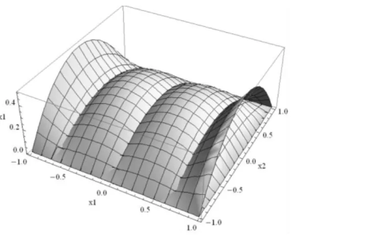
Fig. 2.8. Bivariate Quadratic spline basis functions with one interior knot in dimension x1

and zero interior knots in dimension x2 ... 26

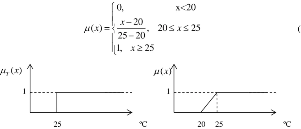
Fig. 2.9. Left: Membership function for a crisp set of ; right: membership function for fuzzy set temperature is hot. ... 29

Fig. 2.10. Example of fuzzy partition with 5 fuzzy sets ... 29 Fig. 2.11.



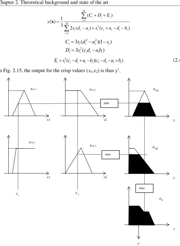
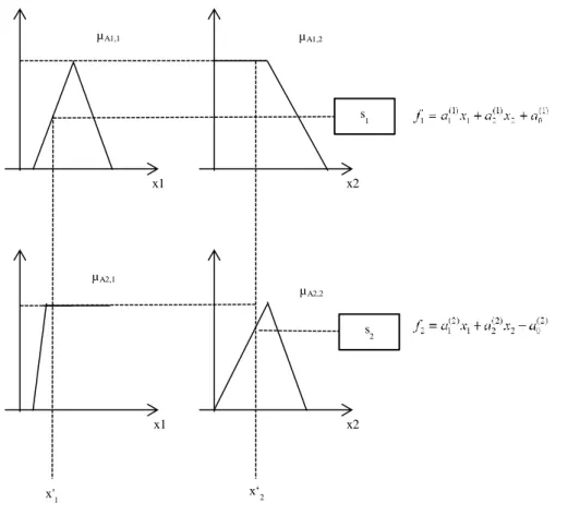
-cuts on a fuzzy set. ... 30 Fig. 2.12. Block diagram of a fuzzy system ... 32 Fig. 2.13. Membership functions for antecedents variables x1 and x2 ... 33

Fig. 2.14. Steps for evaluating a Mamdani-type fuzzy system ... 34 Fig. 2.15. Example of fuzzy inference for a Mamdani-type system with two rules ... 36 Fig. 2.16. Example of fuzzy inference for a TSK model with two rules and two input variables ... 38

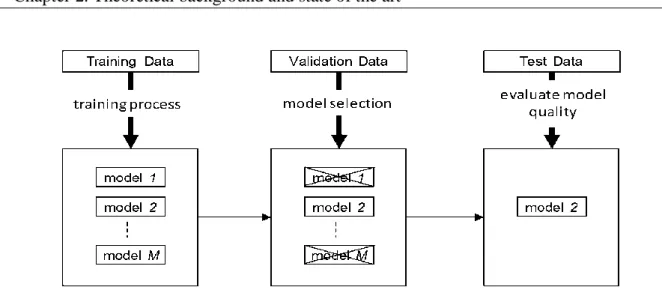
Fig. 2.17.Training, validation and testing of models ... 51 Fig. 2.18. Configuration of a neuro-fuzzy system (after [18]) ... 53 Fig. 2.19. Example of chromosome representation in the GA. ... 63 Fig. 2.20. Mutation in a GA inverts randomly a set of bits in the individual ... 63 Fig. 2.21. One-point crossover operation between two parents. Parents are cut at one point and information of one side is exchanged. ... 64

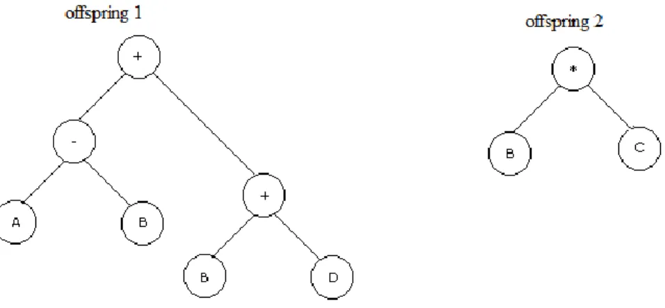
Fig. 2.22. Example of an expression tree ... 67 Fig. 2.23. Parts selected in the parents to participate in the crossover operation ... 68 Fig. 2.24. The resulting ET structures after crossover ... 69

(24)

xxiv

Fig. 2.25. Mutation operation. On the left the original ET structure; on the right, the resulting ET structure after mutation ... 70

Fig. 2.26. Example of an expression tree in genetic programming for B-Splines... 71 Fig. 2.27 A sample expression tree for representing a B-spline network in GP ... 73 Fig. 2.28. Representation of expression (2.130) ... 75 Fig. 2.29. Representation of expression (2.133) ... 76 Fig. 2.30. Representation of expression (2.134) ... 77 Fig. 2.31. Example of a chromosome in BEA ... 79 Fig. 2.32. Bacterial mutation operation ... 81 Fig. 2.33. Bacterial Gene Transfer operation ... 82 Fig. 2.34. Example of a projection based structure. The inputs ui are projected on to the

weight vectors yielding the reduced input set x. The model can be obtained as a function of

m n



input variables. ... 86 Fig. 2.35. ANOVA decomposition employed by the ASMOD algorithm (after Brown and Harris, [57]). ... 88

Fig. 2.36. A hierarchical structure where the model is represented by four subsystems in a cascaded architecture ... 92

Fig. 2.37. Example of typical grid partitioning ... 94 Fig. 2.38. Example of a structure search procedure for the LOLIMOT algorithm for a two-dimensional input space ... 96 Fig. 2.39. Illustration of function integration in one dimension. ... 98 Fig. 3.1. Flowcharts for a) the RBGEN Algorithm; b) the RBMOD algorithm... 114 Fig. 3.2. Example of knot addition ... 115 Fig. 3.3. Example of knot removal restrictions ... 116 Fig. 3.4. The output of the B-Spline Network for the test function and the best candidate, using RBMOD. The red ‘*’ points indicate the specified optima of the function. ... 119

Fig. 3.5. Surface for the fake banana function ... 120 Fig. 3.6. Surface for the paraboloid function ... 120 Fig. 4.1. Outline of Bacterial Programming. ... 125 Fig. 4.2. Mutation on a function part: the individual’s selected node sub-tree is changed randomly. ... 126

Fig. 4.3. Mutation on a terminal part: only the selected node is changed randomly given the terminal mutation rates. ... 127

(25)

xxv

Fig. 4.4. The gene transfer procedure. ... 128 Fig. 4.5. Target output and error vector for the six dimensional generic function problem, using GP. ... 133

Fig. 4.6. Target output and error vector for the six dimensional generic function problem, using BPA. ... 133

Fig. 4.7. Empirical probability distribution function for the pH problem... 134 Fig. 4.8. Empirical probability distribution function for the ICT problem ... 135 Fig. 4.9. Empirical probability distribution function for the generic six dimensional problem ... 135

Fig. 5.1 Evolution cycle for the BPLM algorithm. ... 139 Fig. 5.2 Initial tree structure creation process. A pre-defined BSNN model induces the corresponding tree structure. ... 139

Fig. 5.3 Mutation is performed at the terminal level only: the interior knots’ positions are randomly changed. ... 140

Fig. 5.4 Operation performed during gene transfer. ... 141 Fig. 5.5 Knots and MSE evolution for 100 different initial starting points using the LM algorithm for model 1: ‘*’ specifies the starting point; ‘+’ specifies the final point ... 142

Fig. 5.6 Knots evolution for the 150 different initial positions using the LM algorithm for model 2: ‘*’ specifies the starting point; ‘+’ specifies the final point; local optima are specified by ‘o’. ... 143

Fig. 5.7. Population evolution for model 1... 144 Fig. 5.8. Population evolution for model 2 ... 144 Fig. 5.9. Performance surface seen by BPA when optimizing model 1 ... 145 Fig. 5.10. MSE line for best candidate at every generation when optimizing model 1. .... 146 Fig. 6.1. Possible example of proposed input domain decomposition... 148 Fig. 6.2. Example of a grid partitioning (the same as used by ASMOD algorithm). ... 149 Fig. 6.3. Grid partitioning corresponding to 1 merge of size 2x3; the coloured cells correspond to a possible domain decomposition... 149

Fig. 6.4. Grid partitioning corresponding to 2 merges of size 1x2; the coloured cells correspond to a possible input domain decomposition. ... 150

Fig. 6.5. Grid partitioning corresponding to 1 merge of size 3x1; Notice that this partitioning is not induced by λ

 

S_i . ... 151

(26)

xxvi

Fig. 6.7. Example of input space partitioning ... 152 Fig. 6.8. Spline functions support for a grid with one merge of size 2x1 ... 153 Fig. 6.9. Constant splines representation for a univariate model composed of two univariate submodels, in the same input variable (I_1,1I_1,2I_1,3I_2,1). ... 157

Fig. 6.10. Triangular splines representation for a univariate model composed of two univariate submodels, in the same input variable. ... 158

Fig. 6.11. Triangular splines representation of two univariate submodels, in the same input variable (I1I2I3). ... 159

Fig. 6.12. Triangular splines representation for a bi-dimensional submodel with zero interior knots in dimension x1 and one interior knot in dimension x2. ... 160

Fig. 6.13. Two distinct grid partitions using two merges of the same size; complexity of grid in a) is larger than that of grid in b). ... 164

Fig. 6.14. Sample of a Grid partition with five merges. ... 165 Fig. 6.15. Sample of two grids with two equal merges, but of distinct complexity; the slashed line represents the removed interior knot in merge M1 and M2; triangular splines are considered for dimension x2. ... 165

Fig. 6.16. 3D plot of function f x x



₁, ₂



... 167 Fig. 6.17. A bi-dimensional input space partitioning with: a) one merge (Model_1); b) one merge (Model_2); c) two merges (Model_3); d) two merges (Model_4) ... 168

Fig. 6.18. Training data input-output 3D plot for Base Model, Model_1, Model_2 and Model_3. ... 168

Fig. 6.19. Target versus model output for training and validation sets for Model_1, Model_2, Model_3 and Base Model ... 169

Fig. 6.20. Training data input-output 3D plot for Model_4. ... 169 Fig. 6.21. Model_4 output versus target; top lines: training data; bottom lines: validation set; notice how a misplaced merge induces a big deviation between this model’s output and the target (validation set). ... 169

Fig. 6.22. Another bi-dimensional input space partitioning with two merges (Model_5); functionally speaking, it may be regarded as a model consisting of the sum of 4 sub-models, where each sub-model input domain is delimited by the set of grid cells nominated by circles 1-4. ... 170

Fig. 6.23. Training data input-output 3D plot for Model_5. ... 170 Fig. 6.24. Grid with 2*6 cells ... 173

(27)

xxvii

Fig. 6.25. Example 1 of edge mutation ... 174 Fig. 6.26. Example 2 of edge mutation ... 174 Fig. 6.27. Example 1 of size mutation ... 175 Fig. 6.28. Example 2 of size mutation ... 176 Fig. 6.30. Illustration of the crossover operation ... 177 Fig. 6.30. Approach 2 in the crossover operation ... 177 Fig. 6.30. The 3 possibilities for Approach 3 in the crossover operation ... 178 Fig. 6.31. Plot of training versus validation data: a) training data input x1 versus input x2; b)

validation data input x1 versus input x2; input versus target for training (‘*’) and validation

data (‘o’). ... 181 Fig.6.32. Grid partitioning for the final model of: a) run 1; b) run 2; c) run 3. ... 183 Fig.6.33. left) Target for training input patterns; right) target for validation input patterns ... 186 Fig. 6.34. A sample grid partition for a bivariate model ... 188 Fig. 6.35. The partitioned grid for the first example ... 193 Fig. 6.36. Performance surface for the model given by grid from Fig. 6.29... 193 Fig. 6.37 Final grids after optimizing grid parameters using LM for three distinct initial points ... 196

Fig. 6.38. Plot of x1 versus x3 for the Mackey-Glass time series ... 197

Fig. 6.39. Partitioned grid: a) with 1 merge of size 2*1; b) with 1 merge of size 2*1; c) with one merge of size 3*1; d) with 3 merges of size 3*1 ... 198

Fig. 7.1. Encoding of the fuzzy rules in BEA ... 202 Fig. 7.2. Trapezoidal membership function in the antecedent part of the ith rule ... 203 Fig. 7.3. Outline of the bacterial memetic algorithm ... 206 Fig. 7.4. Decrease of the number of rules in bacterial mutation... 207 Fig. 7.5. Increase of the number of rules in bacterial mutation ... 208 Fig. 7.6 Performance of the LM Method for the pH Problem ... 209 Fig. 7.7. Performance of the BP Method for the pH Problem ... 209 Fig. 7.8 Performance of the LM Method for the ICT Problem ... 210 Fig. 7.9. Performance of the BP Method for the ICT Problem ... 210 Fig. 7.10. The Fuzzy System Parameters Evolution ... 211 Fig. 7.11. MSE Evolution... 212 Fig. 7.12. Performance of the LM Method for the ICT Problem ... 212

(28)

xxviii

Fig. 7.13. Performance of the BP Method for the ICT Problem ... 213 Fig. 7.14. Target and error lines for pH problem using BMA’s candidate with lowest MSE value... 217

Fig. 7.15. Target and error lines for pH problem using BEA’s candidate with lowest MSE value... 217

Fig. 7.16. Target and error lines for ICT problem using BMA’s candidate with lowest MSE value. ... 218

Fig. 7.17. Target and error lines for ICT problem using BEA’s candidate with lowest MSE value... 219

Fig. 7.18. Target and error lines for sixth dimensional problem using BMA’s candidate with lowest MSE value. ... 220

Fig. 7.19. Target and error lines for sixth dimensional problem using BEA’s candidate with lowest MSE value. ... 220

Fig. 7.20. Target and error lines for the agricultural problem using BMA’s candidate with lowest MSE value. ... 221

Fig. 7.21. Target and error lines for the agricultural problem using BEA’s candidate with lowest MSE value. ... 222

Fig. 7.22. Target and error lines for the chemical problem using BMA’s candidate with lowest MSE value. ... 223

Fig. 7.23. Target and error lines for the chemical problem using BEA’s candidate with lowest MSE value. ... 224

Fig. 7.24. MSE line for pH problem ... 225 Fig. 7.25. MSE line for ICT problem ... 225 Fig. 7.26. MSE line for 6 dimensions problem ... 225 Fig. 7.27. MSE line for the agricultural problem ... 226 Fig. 7.28. MSE line for the chemical problem ... 226 Fig. 8.1. Evolution of 4 different trainings with a) LM using Ruano Jacobian (functional version); b) LM using Ruano Jacobian (discrete version); c) LM using Golub-Pereyra

Jacobian (functional version); d) LM using Golub-Pereyra Jacobian (discrete version); e) BP

(functional version); f) BP (discrete version) ... 245 Fig. 8.2. Non-linearity relating the pH concentration with chemical substances ... 250

(29)

xxix

Fig. 8.3. Comparison of input-output plots between the discrete and functional versions, illustrating a better capacity of function approximation by the functional version with different training data sets (from a) till e)) ... 251

Fig. 8.4. Performance surface of a, with 4 different trainings ... 254

Fig. 8.5. Evolution of 4 different trainings using a) Golub-Pereyra LM (analytical version); b) Ruano LM (analytical version)... 255

Fig. 8.6. Performance surface of _d, with 4 different trainings a) with BP; b) with LM 256 Fig. 8.7. Performance surface of f , with 4 different trainings ... 257

Fig. 8.8. Performance surface for the analytical approach ... 261 Fig. 8.9. Plot of target function, with the discrete samples marked by a dot. a) 21 samples resulting from a discretization step of 0.1; b) 101 samples resulting from a discretization step of 0.02; ... 261

Fig. 8.10. Plot of target function, with the discrete samples marked by a dot ... 264 Fig. 8.11. Solid line: Plot of target function; the “+” line corresponds to the input-output plot for the model with optima atvˆ₁ 



0.120, 0.361



; the “*”line corresponds to the input-output plot for the model with optima at vˆ₂  



0.361, 0.120



... 266 Fig. 8.12. Solid line: Plot of target function; the “+” line corresponds to the input-output plot for the discrete model; the “*”line corresponds to the input-output plot for the functional model. Subheading a),b),..d) denotes the final parameters for the training with the 1st, 2nd, …,4th

starting points. ... 266 Fig. 8.13. Output-Input plot for the titration-like curve ... 269 Fig. 8.14. Evolution of trainings for 4 starting points (LM Analytical approach) ... 269 Fig. 8.15. Evolution of trainings for 4 starting points (LM functional approach) ... 270 Fig. 8.16. Evolution of trainings for 4 starting points (LM discrete approach) ... 270 Fig. 8.17. Plot of target function, with the discrete samples marked by a dot ... 272 Fig. 8.18. Drawing of the Input-output plot for the samples used in the training (analytical approach) ... 273

Fig. 8.19. The “+” line corresponds to the input-output plot for the discrete model; the “*”line corresponds to the input-output plot for the functional model. ... 274

Fig. 8.20. The “+” line corresponds to the input-output plot for the discrete model; the “*”line corresponds to the input-output plot for the functional model. ... 274

(30)

xxx

Fig. 8.22. Evolution of 4 different trainings for target function t1(x1,x2): a) with LM

analytical version; b) with LM functional version; c) with LM discrete version. ... 276 Fig. 8.23. Input-Output 3D plot for t2(x) ... 278

Fig. 8.24 Evolution of 4 different trainings for target function t2(x1,x2): a) with LM

analytical version; b) with LM functional version; c) with LM discrete version ... 279 Fig. 8.25 Analytical performance surface ... 284 Fig. 8.26. Gaussian quadrature performance surface ... 285 Fig. 8.27. Discrete performance surface ... 286 Fig.A.1. pH titration like curves. ... 311 Fig.A.2. A two-link Robot arm... 312 Fig.A.3. Mackey-Glass time series for 1000 time instants ... 317 Fig.A.4. Desired output for the a) training data and b) test data sets. ... 318 Fig. B.1. Quadratic splines representation for a univariate model composed of two univariate submodels, in the same input variable (I₁I₂). ... 319

Fig. B.2. 1st derivative of the submodels shown in Fig. B.1. ... 320 Fig. B.3. Quadratic splines representation of two univariate submodels, in the same input variable I1I2I3. ... 322

Fig. B.4. Cubic splines representation of two univariate sub-models, in the same input variable ... 325

Fig. B.5. Cubic splines representation of two univariate submodels, in the same input variable I1I2I3 ... 328

(31)

xxxi

List of algorithms

Algorithm 2.1. Levenberg-Marquardt ... 46 Algorithm 2.2. Local nonlinear optimization steps ... 49 Algorithm 2.3. Genetic Algorithm ... 62 Algorithm 2.4. Genetic Programming ... 67 Algorithm 2.5. Gene Expression Programming ... 74 Algorithm 2.6. Bacterial evolutionary algorithm ... 80 Algorithm 2.7. Asmod ... 88 Algorithm 4.1. BPA algorithm ... 124 Algorithm 6.1. Computation of the Jacobian matrix ... 192

(32)

(33)

xxxiii

List of symbols

, ( )

j i k

N x jth spline function of order k in the ith submodel

, , ( )

j i k n n

N x jth spline function of order k in the nth dimension for the ith submodel

||w|| 2-norm of vector w

Ψa analytical version of the Ψ criterion

ng arity in Gene Expression Programming

ci center for the ith neuron

Ti coding of the ith terminal in an ET

si degree of firing or fire strength for the ith rule

(ᴦ)

v

derivative of the basis functions outputs matrix in respect to the v parameters

Ψd discrete version of the Ψ criterion

Ωd discretized version of Ω

e error function

e error vector

Ψf functional version of the Ψ criterion

Ωf functional version of Ω

gΨ gradient vector for the Ψ criterion

d



g gradient vector for the Ψ criterion in the discrete approach

f 

g gradient vector for the Ψ criterion in the functional approach

gΩ gradient vector for the Ω criterion

d



g gradient vector for the Ω criterion in the discrete approach

f 

g gradient vector for the Ω criterion in the functional approach

hg head length for a chromosome in Gene Expression Programming

H Hessian matrix

Q input points matrix for derivative equalities

P input points matrix for function equalities

x input vector

(34)

xxxiv

( )j i

a ith consequent parameter in the jth rule for a TS FS

( )i x ith input pattern xi ith input variable , i i i k

Sx_λ ith submodel with the set of input variables xi of order ki, and knot vector λi

J Jacobian matrix

JGP Jacobian matrix definition by Golub-Pereyra

JK Jacobian matrix definition by Kaufmann

JR Jacobian matrix definition by Ruano

JΨ Jacobian matrix for the Ψ criterion

j Jacobian vector for the functional approach

f



j Jacobian vector j for the Ψ criterion

ju Jacobian vector j with respect to the u parameters

jv Jacobian vector j with respect to the v parameters

,

i j

 jth interior knot in the ith dimension

, ,

SD i j

 jth interior knot in the ith dimension in submodel SD

Ii,j jth interval in the ith dimension

 learning parameter

w linear weights vector

i

SC list of coordinates for the ith submodel in a merged grid

L lower coordinates for a merge

_

d der

Γ matrix of basis functions derivatives, corresponding to w_d

_ '_{d der}

Γ matrix of basis functions derivatives, corresponding to w'_d

_

d fun

Γ matrix of basis functions outputs, corresponding to w_d

_ 'd fun

Γ matrix of basis functions outputs, corresponding to w'_d

B matrix of restrictions

ᴦ

matrix of the basis functions outputs

Φ matrix of the integral of basis functions, in the functional approach

C matrix of the neurons centers values

MAX

i

x maximum for the ith dimension

,

i j

A

(35)

xxxv

min

i

x minimum for the ith dimension

Ψ modified version of the Ω criterion

Ni number of cells in the ith dimension

Nclones number of clones

Ngen number of generations in a execution of an evolutionary algorithm

Nind number of individuals in a population

Ninf number of infections

n number of input dimensions

ri number of interior knots in the ith dimension

N number of iterations

h number of linguistic terms in the antecedent part of a rule base

mc number of linguistic terms in the consequent part of a rule base

m number of training samples

ˆ

 optimal value for 

ˆu optimal value for u

ˆv optimal value for v

t output target vector

ᴦ

r

partitioned matrix of the basis functions outputs d

Γ partitioned matrix of

ᴦ

, corresponding to wd

'_d

Γ

partitioned matrix of

ᴦ

, corresponding to w'_d

ᴦ

i partitioned matrix of

ᴦ

, corresponding to wi

eP prediction error vector

d(t) real world process output at time instant t.

 regularization parameter for the LM algorithm

R rotation matrix for gradient-based training algorithms

fR



j Ruano’s version of the

f 

j jacobian

ki spline order in the ith dimension

tg tail length for a chromosome in Gene Expression Programming

 

x

t target function in the input variables x

(36)

xxxvi

nu total number of linear parameters

nv total number of nonlinear parameters

nz total number of the model internal parameters

Ω training criterion based on the sum-of-squared-errors

uf u parameters for the functional approach

s[k] update vector in the training algorithms, at the kth iteration

U upper coordinates for a merge

i

 variance for the ith neuron

φ vector of basis functions

i

P

ind vector of indices of the activated basis functions for the P points in the ith submodel

i(t) vector of input signals to a dynamic system at time instant t.

u vector of linear parameters

d

w

vector of linear weights, dependent on the restrictions

'_d

w

vector of linear weights, independent but activated by the restrictions

i

w vector of linear weights, independent of the restrictions

v vector of nonlinear parameters

b vector of restrictions target values

y vector of the model output

z vector of the model’s internal parameters

MAX

x vector specifying the maxima for the input domain

min

x vector specifying the minima for the input domain

X universe of discourse

, ,

SD i j

w weight for the ith univariate function (from the 1st dimension) and the jth

(37)

xxxvii

List of acronyms

1PR 1 Point Recombination

2PR 2 Point Recombination

ABBMOD Adaptive B-Spline Basis Function Modeling of Observational Data

AIC Akaike Information Criterion

AIS Artificial Immune Systems

AMN Associative Memory Network

ANN Artificial Neural Networks

ARMAX AutoRegressive Moving Average with eXogenous input

ARX AutoRegressive with eXogenous input

ASMOD Adaptive Splines Modelling of Observable Data

BAR Balanced Aspect Ratio tree

BBD Balanced Box Decomposition tree

BEA Bacterial Evolutionary Algorithm

BFGS Broyden-Fletcher-Goldfarb-Shanno

BIC Bayesian Information Criterion

BMA Bacterial Memetic Algorithm

BP Error BackPropagation algorithm

BPA Bacterial Programming

BPana Analytical version of error backpropagation

BPd Discrete version of error backpropagation

BPf Functional version of error backpropagation

BPLM Bacterial Programming for Levenberg-Marquardt

BSNN B-Spline Neural Network

BSP Binary Space Partition

CART Classification Adaptive Regression Trees

CI Computational Intelligence

DE Differential Evolution

EA Evolutionary Algorithm

ET Expression Tree

(38)

xxxviii

FS Fuzzy Systems

FUREGA Fuzzy Rule Extraction by Genetic Algorithms

GA Genetic Algorithm

GEP Gene Expression Programming

GFS Genetic Fuzzy System

GMDH Group Method of Data Handling

GP Genetic Programming

ICT Inverse Coordinates Transformation

IS Insertion Sequence

LLM Linear Local Models

LM Levenberg-Marquardt Algorithm

LMana Analytical version of LM

LMd Discrete version of LM

LMf Functional version of LM

LOLIMOT Local Linear Model Tree

MARS Multivariate Adaptive Regression Linear Splines

MC Monte Carlo numerical integration

MF Membership function

MGFS MultiGrid Fuzzy Systems

MLP MultiLayer Perceptron neural network

MSE Mean Square of the absolute Error

MSRE Mean Square of the Relative Error

NARMAX Nonlinear AutoRegressive Moving Average with eXogenous input

NF Neuro-Fuzzy

OLS Ordinary Least Squares

ORF Open Reading Frame

PBGA Pseudo Bacterial Genetic Algorithm

pH pH problem

PMRE Percentage of Mean Relative Error

RBF Radial Basis Function neural network

RIS Reverse Insertion Sequence

RMSE Root Mean Square of absolute Error

(39)

xxxix

SOGP Single Objective Genetic Programming

SONN Self-Organizing Neural Network

SQP Sequential Quadratic Programming

SSE Sum of the Squared Errors

(40)

(41)

1

Chapter 1

1. INTRODUCTION

Among the most important concepts used nowadays by the scientific community is the concept of modeling. The set of tools and methodologies used to design models from experimental data is usually called systems identification. These models can afterwards be employed for different objectives, such as prediction, simulation, optimization, analysis, control, fault detection, etc. Traditionally, the models used are described by mathematical expressions. Examples of these models are Volterra, Wiener series and ARMAX-NARMAX modeling.

More recently, tools and methodologies coming from the Computational Intelligence (CI) area have been applied in Systems Identification. These tools are biologically and linguistically motivated computational paradigms. Examples are Artificial Neural Networks (ANNs) and Fuzzy Systems (FS) which, from the point of view of Systems Identification, are nonlinear models.

Fuzzy systems offer an important advantage over neural networks, which is model transparency. On the other hand, there is an important body of work devoted to training algorithms for neural networks, which are typically gradient-based algorithms. This thesis is focused on Neuro-Fuzzy (NF) models, i.e., models that offer the transparency property, and that can use, for estimation of their parameters, algorithms which were initially proposed for neural networks. One such model is the B-Spline Neural Network (BSNN) and therefore is the model most employed in this work.

Whenever there is a-priori knowledge, it is important to use this knowledge in the model design procedure. This thesis will show how it can be integrated, considering a BSNN model type. One disadvantage of neuro-fuzzy and fuzzy models is that, typically, to obtain a good performance, high-complex models must be used. This work will also present a technique, based on input-domain decomposition, which can result in models with good accuracy, and with reduced complexity.

(42)

Chapter 1. Introduction

2

Evolutionary Algorithms (EAs) are also now recognized tools, in the Systems Identification community, for determining the model structure, which typically can be seen as a combinatorial problem. One recent class of EA algorithms is the Bacterial Evolutionary Algorithm (BEA), which is discussed in this thesis. Combining BEAs and gradient-based algorithms, the Bacterial Memetic Algorithm (BMA) is proposed, which is shown to be a viable tool to design neuro-fuzzy and fuzzy models, both in terms of rule extraction and as a technique to avoid local minima in the training procedure.

Training of ANN and NF models is highly dependent on the data available. This thesis will also propose a methodology whose aim is to decrease the dependence of the training algorithms on the data, focusing on the (typically unknown) mathematical function behind the data.

This chapter starts with brief historical background on the three paradigms from the CI used in this work. Then the basic concepts of system identification are presented, focusing on two of the steps needed for model design that will be covered in this work, namely parameter estimation and model structure selection. Section 1.3 gives an overview of the remaining chapters of this thesis and, the final section of this chapter outlines the contributions of this work.

1.1 Computational intelligence techniques

Computational Intelligence (CI) deals with the theory, design, application, and development of biologically and linguistically motivated computational paradigms emphasizing neural networks, connectionist systems, genetic algorithms, evolutionary programming, fuzzy systems, and hybrid intelligent systems in which these paradigms are contained [http://cis.ieee.org/scope.html]. Further, CI is a collection of computing tools and techniques, shared by closely related disciplines that include fuzzy logic, artificial neural networks, genetic algorithms, belief calculus, and some aspects of machine learning like inductive logic programming [1]. Depending on the type of domain of application these tools are used independently or jointly. The current trend is to develop hybrids of paradigms since no paradigm is superior to the others in every situation.

The following subsections give an overview and historical background on artificial neural networks, fuzzy systems and evolutionary algorithms.

(43)

3

1.1.1 Artificial neural networks

Artificial Neural networks (ANNs) can be regarded as a (very) simplified mathematical model of the human brain in the form of a parallel distributed computing system. To perform a task most ANNs require some form of learning through a process which is similar to training. Typically, they are provided with a training data set which contains information about the behavior of some system, consisting of the inputs of the system and corresponding desired output values. Using adequate training techniques, ANNs can adapt to the environment and learn new associations and new functional associations. Thus, they are seen as promising new generation information processing networks. The key feature of ANNs is that they have the ability to map similar input patterns to similar output patterns [2], characteristic that allows them to have a reasonable generalization capability as well as performing exceptionally well on patterns never previously presented.

In biological Neural Networks, the basic component of brain circuitry is a specialised cell called the neuron. Circuits can be formed by a number of neurons. Any particular neuron has many inputs (some receive nerve terminals from hundreds or thousands of other neurons), each one with different strengths. The neuron integrates the strengths and fires action potentials accordingly.

The input strengths are not fixed, but vary with use. The mechanisms behind this modification are now beginning to be understood. These changes in the input strengths are thought to be particularly relevant to learning and memory.

Donald Hebb (Canadian psychologist) published The Organization of Behavior in 1949 [3]. One of his most important conclusions is drawn from his statement:

“…when an axon of cell A is near enough to excite cell B and repeatedly or persistently takes part in firing it, some growth process or metabolic change takes place in one or both cells such that A's efficiency, as one of the cells firing B, is increased”, which basically means that:

o neurons that fire together are wired, o some mechanism of memory is present, o there is a basic form of learning.

He then introduced a learning rule which tried to explain this associative learning mechanism in biological neural networks. It is probably the oldest learning rule in the artificial neural network field and is denoted as Hebb’s rule.

(44)

4

However, the first neural network that would come to form as a neurocomputer was called the Perceptron and was introduced by Frank Rosenblatt [4] in 1960. He proposed a learning rule for this first basic artificial neural network and proved that, given linearly separable classes, a perceptron would, in a finite number of training trials, develop a weight vector that would separate the classes.

The Perceptron output is a threshold version of the linear combination of its inputs x_i with an additional offset b, often called the bias or offset. Each input is weighted with a corresponding weighted value. The basic rule with this learning model is to change the value of the weights only on active lines and only when an error exists between the network output and the desired output.

At about the same time, Bemard Widrow [5] introduced learning from the point of view of minimizing the mean-square error between the output of a different type of ANN processing element, the ADALINE [6], and the desired output vector over the set of patterns. This work led to modern adaptive filters. Adalines and the Widrow-Hoff learning rule were applied to a large number of problems, probably the best known being the control of an inverted pendulum.

Despite the progress in this area, the biggest setback came when Minsky and Papert began promoting the field of artificial intelligence (what is known nowadays as expert systems) at the expense of neural networks research. They wrote “Perceptrons” [7], a book where it was mathematically proved that these neural networks were not able to compute certain essential computer predicates like the EXCLUSIVE OR Boolean function. It was not until the middle of 1980’s that interest in artificial neural networks re-started to rise substantially, making ANN one of the most active current areas of research, partially to work by Hopfield, Rumelhart [8] and McLelland [9].

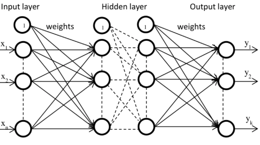
Several different architectures of ANN have been proposed over the years. All of them try, with different degrees, to exploit the available knowledge of the mechanisms of the human brain. Generally, an ANN consists of an input layer, hidden layers and an output layer. At each layer, a pre-defined number of artificial neurons are connected to others in the next layer. A typical ANN structure is shown in Fig. 1.1. These ANN have had numerous applications, including diagnosis, speech recognition, image processing, forecasting, robotics, classification, and many others.

(45)

5

Fig. 1.1. Illustration of an artificial neural network

Among the most studied structures of ANNs are certainly Multi-Layer-Perceptron Networks (MLPs), Radial Basis Function Networks (RBFs) and B-Spline Neural networks, which may be considered neuro-fuzzy systems.

1.1.2 Fuzzy systems

Computing systems use binary encoding to represent the information or knowledge about a problem. Associated with Boolean logic is the traditional two-valued set theory where the element belongs to a class or not, a form of defining precise class membership.

However, a solution to many real-world problems cannot be achieved by mapping the problem domain to two-valued variables. In contrast, they require a representation language that is able to process incomplete, imprecise and vague information. Fuzzy theory provides the formal tools for dealing with such vague information. With fuzzy logic, domains are characterized by linguistic terms instead of numbers. Fuzzy logic provides the tools for dealing with statements such as “it is slightly cold” and “this person is very old”. Thereby, it defines appropriate linguistic terms for “slightly” and “very”, describing the magnitude of the fuzzy variables “cold” and “old”, respectively. The human brain is capable of understanding these statements and infer that probably it is a cloudy day or that a very old person is not a child.

Combining fuzzy logic and fuzzy set theory provides a means to model human reasoning. Furthermore, in fuzzy sets, an element belongs to a set given a degree, indicating the percentage of membership.

The foundation of two-valued logic traces back to 400 BC and is due to research developed by Aristotle and other philosophers of that time, when the first version of Laws of Thought [10], the Law of the Excluded Middle was proposed. This first version stated that every proposition must have only one of two possible outcomes, either true or false.

Output layer Hidden layer

(46)

6

The foundation to what today is referred as fuzzy logic is rewarded to another philosopher, Plato. It was not until the 1900’s that, an alternative to Aristotle’s two-valued logic was proposed by Lucasiewicz [11] and mathematical background on fuzzy theory (infinite valued logic) was produced in 1965 by Lofti Zadeh [12]. His main idea was that most of the phenomena of the real world could not be described by two values, so he defined a function which would assign fuzzy truth degrees between zero and one to elements of a universal set. This way he introduced the mathematical way of representing vagueness in everyday life.

Everyday language is one example of ways of applying vagueness. If one says “the tomato is ripe” or “the tomato is red”, one knows that these are similar concepts. So, a fuzzy concept of uncertainty is associated with the decisions one makes, though from imprecise information. As abovementioned, the main motivation for developing fuzzy systems was the need to represent human knowledge and corresponding decision processes. In the specific case of systems identification, fuzzy rule-based systems are applied where the relations between variables are expressed by if-then rules. Fuzzy sets are then used to represent the ambiguity in the definition of the linguistic terms that form these rules. They are defined by membership functions which map the elements of the considered universe to the interval [0,1]. A value between 0 and 1 defines a partial membership, whereas the extreme values 0 and 1 denote null and complete membership. This partial membership allows one particular element to belong to different fuzzy sets and facilitates a smooth outcome of the reasoning when using fuzzy if-then rules.

1.1.3 Evolutionary algorithms

Evolutionary algorithms (EAs) are inspired by Darwin’s theory of evolution instead of mathematically mimicking a biological process as is the case of ANNs. They are driven by the quest for a solution given a goal. With EAs, the search space S must represent the set of all possible DNA strings in nature. Likewise in living organisms, the search space consists of elements s ∈ S which play the role of the natural genotypes. Thus, it is common practice to refer to S as the genome (or chromosome) and to the elements s, as the genotypes. In the problem space X, the solution candidates (termed phenotypes) x ∈ X are instances of genotypes and are obtained from genotype-phenotype conversion process, . This is similar to nature where an organism is an instance of its genotype formed by embryogenesis. Their ﬁtness is then rated according to objective functions which are subject to optimization and drive the evolution into speciﬁc directions.