REM WORKING PAPER SERIES
Assessing Pension Expenditure Determinants – the Case of
Portugal
Maria Teresa Medeiros Garcia, André Fernando Rodrigues Rocha da Silva
REM Working Paper 068-2019
February 2019
REM – Research in Economics and Mathematics
Rua Miguel Lúpi 20, 1249-078 Lisboa,
Portugal
ISSN 2184-108X
Any opinions expressed are those of the authors and not those of REM. Short, up to two paragraphs can be cited provided that full credit is given to the authors.
1
Assessing Pension Expenditure Determinants – the Case of Portugal
Maria Teresa Medeiros Garcia a,b,*, André Fernando Rodrigues Rocha da Silvaa
a ISEG, Lisbon School of Economics and Management, Universidade de Lisboa,
Portugal
Rua Miguel Lupi, 20,1249-078 Lisboa, Portugal
b UECE (Research Unit on Complexity and Economics) is financially supported
by FCT (Fundação para a Ciência e a Tecnologia), Portugal. This article is part of the Strategic Project (UID/ECO/00436/2019).
* Correspondig author. Tel.: +351 213925993; fax: +351 - 213 971 196.
E-mail addresses: [email protected] (M. T. M. Garcia), [email protected] (A. F. R. R. da Silva)
Abstract
Pension expenditure is a concern for the sustainability of public finances in the European
Union. Therefore, assessing pension expenditure determinants is crucial. This study aims
to disentangle the impact of demographic and economic variables, such as ageing,
productivity, and unemployment, on pension expenditure. Using Portuguese time-series
data, from 1975 to 2014, statistical evidence was found of co-integration between
unemployed people aged between 15 and 64 years old, apparent productivity of labour,
the old-age dependence index and pension expenditure as a share of gross domestic
product. The use of a vector error correction model, with impulse-response functions and
variance decomposition, showed that ageing has an almost insignificant impact in the
long-run, when compared with unemployment and productivity.
JEL Classification: C32, C51, C52, H55
2
Introduction
There is worldwide increasing interest in the analysis of the impact of ageing,
productivity, and unemployment on pension expenditure. European social security
systems are concerned with the rise of pension expenditure which motivated several
reforms including adjusting the age eligibility for a pension benefit and adjusting the size
of the pension benefit (Eurogroup 2016; Eurogroup 2017; European Commission, 2014).
However, public pension systems are expected to experience a pattern of increasing
expenditures from the early years of its existence and until a pension scheme reaches a
state of maturity (Plamondon et al. 2002). After a period of 65 to 70 years, under stable
conditions, the expenditure of a scheme expressed as a percentage of insured earnings
normally stabilizes, since the first generation of young new entrants to the scheme has
passed through the various stages of participation. Indeed, pension schemes mature very
slowly, that is, over many decades (Cichon et al. 2004). Moreover, increasing pension
expenditures are a perfectly normal phenomenon during the maturation phase of national
pension schemes, which lasts several decades. Rising pension expenditures per se are not
necessarily indicative of a financial sustainability issue. Therefore, the design of pension financing systems should accommodate this expected growth of pension expenditure. Indeed, pension privatization policies, implemented in a number of countries, as a
consequence of the concern with the pattern of increasing pension expenditure (World
Bank, 1994), did not deliver the expected results, as coverage and benefits did not
increase, systemic risks were transferred to individuals and fiscal positions worsened
(Beattie and McGillivray, 1995; ILO, 2018). Consequently, several countries are
3 In addition, recent austerity or fiscal consolidation trends affected the adequacy
of pension systems and general conditions of retirement, putting at risk the fulfilment of
the minimum standards in social security and, consequently, the contribution of public
pension systems to the Sustainable Development Goals (SDGs) (ILO, 2017; ILO, 2018).
Few studies are available regarding the factors that influence the evolution of
Portuguese pension expenditure, and whether there is a link between pension expenditure
as a dependent variable and other relevant explanatory variables, including the most
recent developments on relevant variables, covering the current environment and data.
This paper aims to understand which variables have a relevant influence on social
security pension expenditure using econometric techniques that include a vector error
correction model (VECM).
In the next section we describe the Portuguese public pension system. Next we
review the literature covering the impact of ageing on several macroeconomic variables
especially pension expenditure. In the methods section, we present our data and method.
In the following section, we show our estimation results. Last sections provide the
discussion and the conclusion.
The Portuguese Pension System
The Portuguese pension system is an earnings-related public pension scheme with a
means-tested safety net (OECD, 2015), which is financed both by contributions from
employees, employers, and by transfers from the State budget.
Throughout its existence, several measures have been enacted to allegedly reinforce the
pension system’s financial sustainability, such as the creation of the public pension
reserve fund in 1989, and the convergence of the civil servants’ scheme with the public
4 In 2007, a sustainability factor was introduced for the calculation of the old age
pension benefit, reducing it so that it takes life expectancy into account. This was further
changed in 2013, with a decrease in the pension benefit, although this only covered early
retirement. This reform, whose effects will mainly be felt in the medium and long term,
also intended to promote the financial sustainability of the public finances, reducing the
expected value of future pension expenditure and replacement rates. Simultaneously, as
a consequence of the Portuguese bailout in 2011 (European Commission, 2011), a
extraordinary solidarity contribution was also introduced which decreased all pension
income.
In 2013, the normal retirement age was established 66 years in 2014, but increased
to 66 years and two months in 2015, following the automatic process of adjusting the
normal age of retirement by two-thirds of gains in life expectancy from age 65, measured
as the average of the previous two years (Garcia, 2017).
In summary, Portugal essentially has a pay-as-you-go pension scheme (World
Bank, 2006), which represents the major source of retirement income, with occupational
and personal pension funds only existing to a minor extent (Blake, 2006; European
Parliament, 2011; Garcia, 2017). The Portuguese system is also a defined-benefit system
(European Commission, 2015), offering pensioners more measurable post-employment
income benefits (Ramaswamy, 2012). Pensions are indexed to prices and gross domestic
product (European Commission, 2015).
Literature Review
Demographic aging and its impact on pension expenditure brought to the debate the need
5 Roach and Ackerman (2005) show that a wide range of existing policy options
could be used to secure the finances of the U.S.A. social security programme over the
next 75 years without major structural changes, whereby it will continue to provide
beneficiaries with a stable and predictable source of retirement income. These authors
believe that the system is not in crisis and that it cannot go bankrupt as long as revenues
continue to be collected.
Ramaswamy (2012) stress the ideas that lower payroll tax revenues during a
period of high unemployment and rising fiscal deficits are a test of the sustainability of
pay-as-you-go public pension schemes, as well as poor financial market returns and low
long-term real interest rates, which create challenges for the defenders of defined benefit
pension schemes.
To limit public expenses, pension benefits might be decreased, however
retirement income adequacy is a concern (European Parliament, 2011; Chybalski and
Marcinkiewicz, 2014). Orenstein (2011) calls attention to the fact that, from 1981 to 2007,
more than thirty countries worldwide fully or partially replaced their pre‐existing pay‐as‐ you‐go pension systems with ones based on individual, private savings accounts in a process often labelled “pension privatisation”. However, pension privatization did not
deliver the expected results (ILO, 2018), revealing limited effects on capital markets and
economic growth. In fact, coverage rates and pension benefits decreased, the risk of
financial market fluctuations was shifted to individuals, and administrative costs
increased. Moreover, the high costs of transition created large fiscal pressures. In
addition, private pension fund administration did not improve governance as, frequently,
the regulatory and supervisory functions were captured by economic groups responsible
6 Cipriani (2014) uses an overlapping generations model with a pay-as-you-go
pension system to conclude that population ageing due to increased longevity implies a
reduction in pension benefits. However, the effects of aging on pensions may not be
negative if the elderly are free to choose their retirement age, while they are always
negative in the case of full retirement (Cipriani, 2016).
Halmosi (2014) emphasises that the study of the pension systems of developed
countries is a priority issue in light of the 2008 economic crisis. Grech (2015) presents
evidence that the impacts of the crisis were different for continental and Mediterranean
systems, where pension benefits of the later were cut back significantly.
Natali and Stamanti (2014) analysepension reforms in Greece, Italy, Portugal, and
Spain, between, 1990 and 2013, concluding that all countries encouraged the spread of
private pensions and harmonised their fragmented public schemes. In addition, cost
containment was massive, putting future adequacy at risk.
Natali (2015) provides a summary of reforms in Europe since the onset of the Great
Recession, showing that evidence proves that austerity has hit both public pay-as-you-go
schemes and private pre-funded schemes alike. Indeed, both have been subject to
measures to contain costs (e.g., a higher pensionable age, the introduction of automatic
stabilisers of future spending, reduced indexation, and higher taxes and/or contributions).
Indeed, Diamond (1996), much earlier, suggested the indexation of normal retirement age
to life expectancy, and the investment of part of the public reserve funds in the private
economy as being good measures to solve the social security pension system problem.
Bloom et al. (2010) analyse the implications of population ageing for economic
growth, concluding that the results suggest that OECD countries are likely to see modest
7 reforms (including an increase in the legal age of retirement) can mitigate the economic
consequences of an ageing population.
In order to disentangle the macroeconomic impacts on the pay-as-you-go
Portuguese social security system, Garcia and Lopes (2009) conclude that some
cumulative measures such as a changing of indexing rules, a better actuarial match
between pensions and contributions, and measures to increase the effective age of
retirement, could have a bigger impact on reducing the expected increase in pension
expenditure than applying a systemic pension reform. Using a macroeconomic model of
the Portuguese economy, the estimations suggest that the elimination of early retirement
schemes, combined with an increase in the effective contribution rate could be a good
alternative to promote the financial sustainability of the system. Economic growth
strengthened by the pension reserve fund (which had an average annual nominal rate of
return of 5.17% during the period 1989-2014, and relatively low administrative costs
compared with funded systems), brings more advantages to the system when compared
with a fully pre-funded system, which has high transition costs, with current tax payers
being responsible for paying both their own and the existing pensioners benefits
(European Parliament, 2011).
This paper analyses the factors that influence the evolution of Portuguese pension
expenditure, including the most recent developments on relevant variables.
Methods
Sample
In order to study the determinants of pension expenditures, we adopt the ratio between
pension spending and gross domestic product at current prices as the dependent variable
8 The independent variables consider eight factors that might influence pension
expenditure. The first group of factors follows the related literature concerning the
macroeconomic and demographic characteristics:
(1) Unemployment consists of unemployed people defined as someone aged 15 to 64
without work during the reference week, available to start work within the next
two weeks (or has already found a job to start within the next three months), and
has actively sought employment at some time during the last four weeks. In
pay-as-you-go systems, the unemployment shrinks the contribution base, negatively
affecting the pension system balance.
(2) Apparent labor productivity denotes apparent productivity of labor that relates
the wealth created to the labor factor. The apparent labor productivity is the real
gross domestic product in terms of expenditure, at constant prices of 2011, per
annual hours worked by employed people. Apparent labor productivity presents
the potential to overcome the negative effects of ageing, positively affecting the
pension system balance.
(3) Old age dependency ratio is the ratio between elderly people at an age when they
are generally economically inactive (i.e. aged 65 and over) and the number of
people of working age (i.e. 15 - 64 years old). This variable is expected to have a
positive effect on the dependent variable.
The second group tries to disentangle the impact of the main pension system laws
since 1975 (Garcia, 2017). Therefore, five dummy variables were set, each of which refers
to a specific period, that is to say, the variable’s value will be 1 if included in that specific
9 (4) Revolution of April 1974, which led to important social and economic changes
during the second half of the ‘70s. This variable is expected to have a positive
effect on the dependent variable.
(5) The first Social Security Act of 1984, which established pension benefit payments
in the private sector. This variable is also expected to have a positive effect on the
dependent variable.
(6) The Social Security Reform of 1993, which made changes to the social security
system of the Public Administration (civil servants), in order to be similar with
that of the private sector. This reform considers a new formula for the calculation
of public employees’ pensions, which is the same as that of the private sector
workers’ scheme. This variable is expected to have a negative effect on the dependent variable.
(7) The Third Social Security Act of 2002, which considered parametric changes to
the old age pension benefit formula, including the accrual rate and life-time
earnings. This variable is expected to have a negative effect on the dependent
variable.
(8) The Fourth Social Security Act of 2007, which introduced the sustainability factor
and the voluntary public regime of capitalisation. The sustainability factor is the
ratio between average life expectancy at the age of 65 in 2000 and average life
expectancy at the age of 65 for the year prior to the year for which the pension
benefit is calculated. This Act also increases the penalty for early retirement to
6% per year. This variable is also expected to have a negative effect on the
10 We conduct linear regression analysis using annual time series data from 1974 to
2015. The equation of the model is:
(1)𝑌𝑡 = 𝛽0+ 𝛽1𝑋1𝑡+ 𝛽2𝑋2𝑡+ 𝛽3𝑋3𝑡+ 𝛿0𝐷1𝑡+ 𝛿1𝐷2𝑡 + 𝛿2𝐷3𝑡+ 𝛿3𝐷4𝑡+ 𝛿4𝐷5𝑡+ 𝜀𝑡
Where 𝑌 is the ratio between pension spending and gross domestic product; 𝑋1 is the unemployment in logarithmic form; 𝑋2 is the apparent labor productivity in
logarithmic form; 𝑋3 is the old age dependency ratio; and 𝐷1 to 𝐷5 represent dummy
explanatory variables used to indicate the occurrence of the events described above.
(1) 𝑝𝑒𝑛𝑠𝑖𝑜𝑛𝑠
𝑔𝑟𝑜𝑠𝑠 𝑑𝑜𝑚𝑒𝑠𝑡𝑖𝑐 𝑝𝑟𝑜𝑑𝑢𝑐𝑡𝑡
= 𝛽0+ 𝛽1𝑙𝑜𝑔 𝑢𝑛𝑒𝑚𝑝𝑙𝑦𝑚𝑒𝑛𝑡𝑡+ 𝛽2𝑙𝑜𝑔 apparent labor productivity𝑡 + 𝛽3𝑜𝑙𝑑 𝑎𝑔𝑒 𝑑𝑒𝑝𝑒𝑛𝑑𝑒𝑛𝑐𝑦 𝑟𝑎𝑡𝑖𝑜𝑡+ 𝛿0𝑅𝑒𝑣1974𝑡+ 𝛿1𝑅1984𝑡
+ 𝛿2𝑅1993𝑡+ 𝛿3𝑅2002𝑡+ 𝛿4𝑅2007𝑡+ 𝜀𝑡 The data sources are PORDATA and OECD.
Descriptive statistics for the variables used in the analysis are presented in the
appendix (Table A1).
Analysis
To test for stationarity, unit root tests were undertaken (Wooldridge, 2009). Following
the methodology adopted by Brooks (2014), the tests used were the Augmented
Dickey-Fuller test and Phillips-Perron test. The p-values analysis of both tests suggests that the
null hypothesis of the presence of a unit root cannot be rejected in all variables at 10%
significance level, and that stationarity is achieved with first differences through the
rejection of the same null hypothesis at 5% significance level, highlighting their strong
persistence (I(1) process).
The finding of non-stationarity may render the potential econometric results
11 is desirable to obtain I(0) residuals, which are only achieved if the linear combination of
I(1) variables is I(0), that is to say, if the variables are co-integrated (Brooks, 2014).
With regards to the hypothesis of the existence of more than one linearly
independent co-integration relationship between more than two variables, it is appropriate
to stress the issue of co-integration using the Johansen VAR test. To develop the Johansen
VAR framework, the selection of the optimum number of lags is needed to avoid
problems of residual autocorrelation, using the VAR Lag Order Selection Criteria
procedure. The Likelihood Ratio Criteria (LR), the Final Predictor Error (FPE), and the
Hannan-Quinn Information Criteria (HQ) selected two lags as an optimum limit, against
the evidence of the Akaike Information Criteria (AIC) and the Schwarz Information
Criteria (SC), which presented the optimum selection of three and one lag, respectively.
The Johansen co-integration test allows for the selection of the appropriate lag
length and model to choose. The test result suggests that the number of appropriated lags
is two (as referred before), with one co-integrating vector, and the model to adopt consists
of the allowance of a quadratic deterministic trend, with intercept and trend in the
co-integration equation and intercept in VAR, following Akaike Information Criteria
(Brooks, 2014).
Therefore, it was decided to use an error correction model “incorporated” into a
VAR framework in order to model the short and long-run relationships between variables:
a Vector Error Correction Model (VECM). The VECM can be set up in the following
form (Brooks, 2014):
(2) ∆𝛾𝑡= П𝛾𝑡−𝑘+ 𝛤1∆𝛾𝑡−1+ ⋯ + 𝛤𝑘−1∆𝛾𝑡−(𝑘−1) + 𝑢𝑡 where П= (Σ𝑖=1𝑘 𝛽𝑖) − 𝐼𝑔 and 𝛤𝑖 = (𝛴𝑗=1𝑖 𝛽𝑗) − 𝐼𝑔.
12 This VECM contains g variables in first-differenced form on the LHS, and k-1
lags of the dependent variables (differences) on the RHS, each with a Γ short-run coefficient matrix. П consists of a long-run coefficient matrix, as being in equilibrium, all the ∆𝛾𝑡−𝑖= 0, and setting 𝐸(𝑢𝑡) = 0 will leave П𝑦𝑡−𝑘= 0. П illustrates the speed of
adjustment back to equilibrium, that is to say, it measures the proportion of last period´s
equilibrium error that it is corrected for (Brooks, 2014).
The VECM model estimation is depicted in Table 1 and encompasses the
co-integration equation with dummy variables.
Table 1. VECM estimation
Cointegrating Eq: CointEq1
Sample (adjusted): 1978 to 2014
Included observations: 37 after adjustments Standard errors in ( ) & t-statistics in [ ]
Determinant residual covariance (dof adj.) 9.01E-11 Determinant residual covariance 9.35E-12 Log likelihood 259.8113
Akaike information criterion -10.36818 Schwarz criterion -7.407571
Pensions to gross domestic
product ratio (-1) 1.000000 Log unemployment (-1) -0.934243 (0.08485) [-11.0107] Log apparent labor
productivity (-1) -3.450917 (0.61569) [-5.60500] Old age dependency ratio (-1)
-0.114074 (0.07355) [-1.55089] @TREND(75) 0.024757 C 18.19483 Error Correction: D(Pensions to gross domestic product ratio)
D(Log unemployment) D(Log apparent labor productivity) D(Old age dependency ratio) CointEq1 -0.823727 (0.25145) [-3.27589] 0.355044 (0.27994) [1.26830] -0.085035 (0.02454) [-3.46495] -0.229154 (0.19648) [-1.16627] D(Pensions to gross domestic
product ratio (-1)) 0.048722 (0.23937) [0.20354] -0.134046 (0.26649) [-0.50301] 0.037997 (0.02336) [1.62640] 0.216371 (0.18705) [1.15678] D(Pensions to gross domestic
product ratio (-2)) -0.023504 (0.19428) [-0.12098] -0.327028 (0.21629) [-1.51196] 0.023747 (0.01896) [1.25233] 0.140985 (0.15181) [0.92867] D(Log unemployment (-1)) 0.402031 (0.24351) [1.65098] 0.652833 (0.27110) [2.40812] -0.002592 (0.02377) [-0.10904] 0.147807 (0.19028) [0.77679] D(Log unemployment (-2)) -0.006098 (0.24210) [-0.02519] 0.136222 (0.26952) [0.50542] -0.054351 (0.02363) [-2.30024] -0.148583 (0.18918) [-0.78542] D(Log apparent labor
productivity (-1)) -0.221389 (2.35803) [-0.09389] 3.246082 (2.62517) [1.23652] -0.463845 (0.23014) [-2.01547] -1.234411 (1.84257) [-0.66994] D(Log apparent labor
productivity (-2)) 0.580083 (1.60695) [0.36098] 0.776474 (1.78900) [0.43403] -0.055980 (0.15684) [-0.35693] -0.496768 (1.25567) [-0.39562]
13
D(Old age dependency ratio (-1)) 0.170345 (0.26139) [0.65169] -0.345219 (0.29100) [-1.18632] 0.035069 (0.02551) [.37463] 0.468223 (0.20425) [2.29241] D(Old age dependency ratio
(-2)) 0.371367 (0.20938) [1.77363] -0.035296 (0.23310) [-0.15142] 0.046423 (0.02044) [2.27169] 0.150022 (0.16361) [0.91694] C -0.066069 (0.13892) [-0.47559] -0.010129 (0.15466) [-0.06550] 0.001324 (0.01356) [0.09766] -0.066055 (0.10855) [-0.60851] @TREND(75) 0.007064 (0.01497) [0.47172] 0.012654 (0.01667) [0.75905] -0.001357 (0.00146) [-0.92828] 0.003988 (0.01170) [0.34082] REV1974 -0.268243 (0.13658) [-1.96393] -0.002228 (0.15206) [-0.01465] 0.053747 (0.01333) [4.03186] 0.162941 (0.10673) [1.52670] R1984 0.077589 (0.11939) [0.64988] -0.199898 (0.13292) [-1.50395] 0.054140 (0.01165) [4.64628] 0.244170 (0.09329) [2.61728] R1993 -0.383299 (0.17433) [-2.19869] 0.032310 (0.19408) [0.16648] -0.040317 (0.01701) [-2.36955] -0.117924 (0.13622) [-0.86567] R2002 -0.099864 (0.16839) [-0.59306] -0.004149 (0.18746) [-0.02213] 0.002105 (0.01643) [0.12808] -0.144916 (0.13158) [-1.10136] R2007 0.169199 (0.10280) [1.64589] -0.040558 (0.11445) [-0.35438] 0.000708 (0.01003) [0.07054] 0.179928 (0.08033) [2.23988] R-squared 0.685045 0.413290 0.802777 0.842369 Adj. R-squared 0.460078 -0.005789 0.661903 0.729776 Sum sq. resids 0.304910 0.377908 0.002904 0.186175 S.E. equation 0.120497 0.134148 0.011760 0.094157 F-statistic 3.045086 0.986188 5.698563 7.481515 Log likelihood 36.27442 32.30368 122.3691 45.40105 Akaike AIC -1.095914 -0.881280 -5.749681 -1.589246 Schwarz SC -0.399301 -0.184667 -5.053068 -0.892633 Mean dependent 0.124324 0.023130 0.020237 0.367568 S.D. dependent 0.163987 0.133761 0.020226 0.181129
As all inverse roots of characteristic polynomial are inside the unit circle, the
model is stable. The residuals assumptions were tested, and it is possible to conclude that
the mean of the residuals is zero. The White Heteroscedasticity test p-value does not allow
for the rejection of homoscedastic residuals. In addition, the covariance between residuals
and explanatory variables is zero, thus satisfying the assumption of there being no
14 hypothesis of no residual serial correlation is not rejected at 5% significance level with
the use of two lags.
As such, the estimators are efficient, and the confidence intervals and hypothesis
tests using t and F-statistics are reliable.
Results
The results suggest that the long-run relationship between
pensions to gross domestic product ratio and old age dependency ratio is negative, whereas the long-run relationship between pensions to gross domestic product ratio and
the other two variables (log unemployment and log apparent labor productivity) is
positive. In fact, the normalised co-integrating model estimation (Table A.2 in the
appendix), without dummy variables, allows one to obtain the following equation:
(3) Pensions to gross domestic product ratio = 1.320370 log unemployment + 1.818858 log apparent labor productivity - 0.221652 old age dependency ratio
The presence of a co-integrating vector illustrates an equilibrium phenomenon, as
it is possible that co-integrated variables may deviate from their relationship in the short
run, but that their association would return in the long run (Brooks, 2014).
Discussion
The positive long-run coefficient of log unemployment suggests that unemployment has
a positive impact on pension system expenditure, which is in line with the literature. High
unemployment leads to negative migratory balances (mostly affecting young people),
aggravating the ageing process, and consequently the declining demographics. With less
people, investment decreases, shrinking the economic growth. The causality from ageing
and unemployment to productivity are confirmed by a VEC Granger Causality Test, at
15 The positive long-run coefficient of log apparent labor productivity on pensions
to gross domestic product ratio is not in line with the European Commission (2015).
Concerning the negative coefficient of old age dependency ratio, this might be the
consequence of the parametric changes introduced to the system since 2000 (Garcia,
2017), especially the one that changed the normal retirement age (NRA) to 66 years old,
in 2013, becoming life expectancy-dependent after 2014. Therefore, an increase of old
age dependency ratio does not compulsorily imply an increase of pension expenditure as
a share of gross domestic product in the long-run. This measure is strongly supported by
the literature as a crucial measure to guarantee the financial sustainability of pension
systems, smoothing the impact of an ever-increasing number of pensioners (Diamond,
1996; Clements et al., 2015). The introduction of a sustainability factor into the benefit
calculation formula, which is related to the evolution of average life expectancy (ALE),
also represents a significant decrease in the pension benefit.
With regards to the short-run coefficients of the dummy variables, only the
revolution of April 1974 (at 10% significance level) and the 1993 Social Security Reform
(at 5%) present statistical significance, and the negative coefficients illustrate each
contribution to the decrease of pension expenditure as a share of gross domestic product,
where the possible causes can be the high average real gross domestic product growth
rate after 1976 until 1979 of 5.4% in the first case (PORDATA), and in the latter case,
the implementation of the same official retirement age between men and women, as well
as the increase of the minimum contributory period from 10 to 15 years.
Finally, the impulse-response functions were stressed, as well as the variance
decomposition for pensions to gross domestic product ratio, which is strongly dependent
16 In order to guarantee some consistency and reasonability of the results, the order
considered was from the most exogenous variable to the most endogenous one,
determined by a VEC Granger Causality Test. The higher the p-value, the greater the
exogeneity of the variable. The adopted order is as follows: old-age dependency ratio, log
unemployment, pensions to gross domestic product ratio and log apparent productivity of
labour.
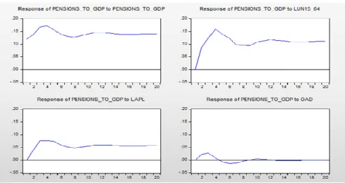
Figure 1. Response to cholesky one standard deviation innovation
Following Brooks’ (2014) methodology, Figure 1 gives the impulse responses for
pensions to gross domestic product ratio, regarding several unit shocks to old-age
dependency ratio and log unemployment and their impact during 20 periods (years)
ahead. Considering the signs of the responses, innovations to old-age dependency ratio
have a positive impact until the 5th year, achieving its peak in the 3rd year. After this, the
impact is negative, although the effect of the shock ends up dying down. A standard
deviation shock to log unemployment and log apparent productivity of labour always has
a positive impact on pensions to gross domestic product ratio, reaching its peak in the 4th
and 3rd years, respectively, and stagnating in the long-run. Finally, the own innovations
17 unemployment, that is to say, it reaches its peak in the 4th year, and then stagnation
thereafter.
When analysing this approach, the main highlight is the fact that old-age
dependency ratio registers an almost irrelevant contribution for the evolution of pensions
to gross domestic product ratio in the long-run, when compared with the other variables,
which is surpassed by the contributions of log unemployment and log apparent
productivity of labour, this reinforcing the doubts about the contribution of ageing on
pension expenditure. It is also possible to verify the relevance of unemployment in the
presence of a positive shock immediately in the first years (as stressed by the European
Commission (2015)), over a 20-year forecasting horizon (positive but constant impact),
shrinking the contributory base and the economic growth, with a similar pattern in relation
to the apparent productivity of labour, guaranteeing higher pension entitlements.
The results of the variance decomposition for the pensions to gross domestic
product ratio residuals show that, for the 20-year forecasting horizon, the old-age
dependency ratio shocks account for only 2.86%, in the first year, and 5.35%, in the 20th
year, of the variance of the pensions to gross domestic product ratio, while log
unemployment contributes between 57.87% and 85.83%, reinforcing the huge importance
of unemployment on pension expenditure and the reduced impact of ageing when
compared with the other variables. It is also important to stress the own shocks of
pensions to gross domestic product ratio, which accounts for between 39.76% and 0.93%
of its movements.
Limitations
The negative relationship between pensions to gross domestic product ratio and old age
18 co-integration test with dummy variables was carried out, although there is a problem in
that the critical values may not be valid with exogenous series, such as dummy variables.
With this test, the old age dependency ratio long-run coefficient becomes positive
and the sign of the other two coefficients does not change. However, it is important to
take into account the econometric limitations of this change. To derive the VECM
p-values, the VECM model with the coefficients as C(1) until C(16) was developed. C(1)
is the coefficient of the co-integration equation (as well as the speed of adjustment back
to equilibrium), C(10) is the constant, C(2) up to C(9) are the short-run coefficients of the
lagged variables (until the second lag), and C(12) until C(16) are the coefficients of the
dummy variables. C(11) is the trend coefficient (Brooks, 2014).
Looking at C(1), which is negative and statistically significant at 5%, this confirms
the long-run relationship between pensions to gross domestic product ratio, log
unemployment, log apparent labor productivity, and old-age dependency ratio, as well as
the existence of a correction mechanism of deviations (Wooldridge, 2009). When
carrying out the Wald Tests, it is not possible to reject the null hypothesis of C(4)=C(5)=0,
C(6)=C(7)=0 and C(8)=C(9)=0, and the conclusion that needs to be stressed is the
absence of short-run causality running from log unemployment,
log apparent labor productivity, and old age dependency ratio to pensions to gross domestic product ratio.
In addition, the results need to be analysed carefully: if the order of variables
changes, then the results of impulse-response functions and variance decomposition can
change drastically, mainly the variance decomposition between pensions to gross
domestic product ratio and log unemployment. Nevertheless, it is noticeable that
19
Conclusion
The results of the estimation, after taking into consideration certain aspects such as
non-stationarity, co-integration, and residuals testing, suggest that unemployment, apparent
productivity of labour, and old-age dependency ratio all jointly present a long-run
relationship with pension expenditure as a share of gross domestic product, but not in the
short-run.
Unemployment is crucial to explain the increase of pension expenditure as a share
of gross domestic product, as reinforced by the review of the literature on pensions. This
interpretation is confirmed by the variance decomposition of pensions to gross domestic
product ratio and also the impulse-response functions.
The apparent productivity of labour also seems to have a positive impact on
pension expenditure to gross domestic product, which is not in line with the European
Commission (2015), supporting the assumption that gross domestic product growth is
larger than pension expenditure growth in Portugal, due to the fact that pensions are not
fully indexed to wages after retirement.
The most intriguing result concerns the old-age dependency ratio. In fact, after the
development of the Johansen co-integration tests, both without dummy variables and with
dummy variables, the old-age dependence ratio long-run coefficient presents different
signs, giving rise to the hypothesis that ageing may not be the most relevant factor which
jeopardises the financial sustainability of the Portuguese public pension system. This fact
is corroborated by the irrelevant influence of old-age dependency ratio (in the long-run)
on the impulse-response-functions.
When designing a pension system policy to reinforce its financial sustainability,
20 increasing demographic strain seems not to impact pension expenditure as critically as
unemployment. Therefore, policies to reduce unemployment should be considered as
policy options to control pension expenditure, which represents a brand new way to
address the financial sustainability of public pension systems.
References
Barr, N. and Diamond, P. A. 2006. The economics of pensions. Oxford Review of
Economic Policy, Vol. 22. No 1. pp. 15-39.
Beattie, R. and McGillivray, W. 1995. A risky strategy: Reflections on the World Bank
Report Averting the old age crisis, International Social Security Review, Vol. 48,
No. 3–4, pp. 5–23.
Blake, D. 2006. Pension Economics. John Wiley & Sons.
Bloom, D. E., Canning, D. and Fink, G. 2010. Implications of population ageing for
economic growth. Oxford Review of Economic Policy, Volume 26, Number 4,
2010, pp. 583–612.
Brooks, C. 2014. Introductory econometrics for finance. 3rd Ed. Cambridge: Cambridge
University Press.
Chybalski, F. and Marcinkiewicz, E. 2014. How to measure and compare pension
expenditures in cross-country analyses? Some methodological remarks.
International Journal of Business and Management. Vol. 2. No 4. pp. 44-59.
Cichon, M.; Scholz, W.; van de Meerendonk, A.; Hagemejer, K.; Bertranou, F.;
Plamondon, P. (2004). Financing social protection, Quantitative Methods in Social
Protection Series Geneva, International Labour Office/International Social Security
21 Cipriani, G.P. 2014. Population aging and PAYG pensions in the OLG model. Journal of
Population Economics. Vol.27. pp. 251-256.
Cipriani, G.P. 2016. Aging, Retirement and Pay-As-You-Go Pensions. IZA DP No. 9969,
May.
Clements, B, Dybczak, K., Gaspar, V., Gupta, S., and Soto, M. 2015. The Fiscal
Consequences of Shrinking Populations. IMF Staff Discussion Note.
Diamond, P. A. 1996. Proposals to Restructure Social Security. Journal of Economic
Perspectives. Vol. 10. No 3. pp. 67–88.
Eurogroup 2016. Common principles for strengthening pension sustainability. 16 June
2016.
Eurogroup 2017. Structural reform agenda - thematic discussions on growth and jobs:
benchmarking pension sustainability. 144/17, 20.3.2017.
European Commission 2011. The Economic Adjustment Program of Portugal, DGEFA
Occasional Paper Nº79, June.
European Commission 2012. The 2012 Ageing Report (Online). Available from:
http://ec.europa.eu/economy_finance/publications/european_economy/2012/pdf/e
e-2012-2_en.pdf
European Commission 2014. Identifying fiscal sustainability challenges in the areas of
pension, health care and long-term care policies. Directorate-General for Economic
European Commission 2015. The 2015 Ageing Report (Online).
European Parliament 2011. Pension Systems in the EU – Contingent Liabilities and Assets
22 Francisco Manuel dos Santos Foundation. (2010). PORDATA, the database of
contemporary Portugal. Retrieved from http://www.pordata.pt/en/Portugal.
Garcia, M. T. M. 2017. Overview of the Portuguese Three Pillar Pension System,
International Advances in Economic Research, 23: 175-189. Published online: 21
April 2017. DOI 10.1007/s11294-017-9636-x.
Garcia, M. T. M. and Lopes, E. G. 2009. The macroeconomic impact of reforming a
PAYG system: The Portuguese Case. International Social Security Review. Vol.
62. No 1. pp. 1-23.
Grech, A. G. 2015. Convergence or divergence? How the financial crisis affected
European pensioners. International Social Security Review. Vol. 68. No 2. pp.
43-61.
Halmosi, P. 2014. Transformation of the Pension Systems in OECD Countries after the
2008 Crisis. Public Finance Quarterly. No 4. pp. 457-469.
ILO, 2017. World Social Protection Report 2017–19: Universal social protection to
achieve the Sustainable Development Goals, International Labour Office – Geneva.
ILO, 2018. Social protection for older persons: Policy trends and statistics 2017–19,
Social Protection Policy Papers, Paper 17, International Labour Office, Social
Protection Department. - Geneva: ILO, 2018.
Natali, D. 2015. Pension Reform in Europe: What has happened in the Wake of the
Crisis? CESifo DICE Report 2/2015 (June), pp 31-35.
Natali, D. and Stamati, F. 2014. Reassessing South European pensions after the crisis:
Evidence from two decades of reforms. South European Society and Politics. Vol.
19. No 3. pp. 309-330.
23 Orenstein, M. A. 2011. Pension Privatization in Crisis: Death or Rebirth of a Global
Policy Trend? (July‐September 2011). International Social Security Review, Vol. 64, Issue 3, pp. 65-80,. Available at SSRN: https://ssrn.com/abstract=1879020 or
http://dx.doi.org/10.1111/j.1468-246X.2011.01403.x
Plamondon, P., Drouin, A., Binet, G., Cichon, M. McGillivray, W.R., Bédard, M., e
Perez-Montas, H. (2002): Actuarial practice in social security, Quantitative
Methods in Social Protection Series, Geneva, International Labour
Office/International Social Security Association, 2002.
Ramaswamy, S. 2012. The Sustainability of Pension Schemes. BIS Working Papers No
368, Monetary and Economic Department, January.
Roach, B. and Ackerman, F. 2005. Securing Social Security: Sensitivity to Economic
Assumptions and Analysis of Policy Options. GDAE Working Paper No. 05-03, ©
Copyright 2005 Global Development and Environment Institute, Tufts University.
Wooldridge, J. M. 2009. Introductory Econometrics, A Modern Approach, 4th Ed.
Boston: South-Western.
World Bank Policy Research Report, 1994. Averting the Old Age Crisis, Policies to
Protect the Old and Promote Growth, Oxford University Press.
Appendix
Table A1. Descriptive statistics
Variables Mean Median Maximum Minimum Std. Dev Skewness Kurtosis Jarque-Bera Dependent variable
Pensions to gross domestic product ratio
5.05 5.15 7.70 2.20 1.28 0.16 2.82 0.28 (0.89) Independent variables
Log unemployment 12.75 12.72 13.66 12.09 0.38 0.65 3.14 2.82 (0.24)
24
Log apparent labor productivity
2.69 2.77 3.01 2.18 0.28 -0.53 2.03 3.43 (0.18) Old age dependency
ratio
22.35 22.00 30.70 16.30 4.09 0.33 1.94 2.61 (0.27) Number of observations 40
The probability is between brackets
Table A2. Johansen Co-integration Test without Dummy Variables
Sample (adjusted): 1978 2014
Included observations: 37 after adjustments Trend assumption: Quadratic deterministic trend
Series: Pensions to gross domestic product ratioLog unemploymentLog apparent labor productivityOld age dependency ratio Lags interval (in first differences): 1 to 2
Unrestricted Co-integration Rank Test (Trace) Hypothesized No. of CE(s)
Eigenvalue
Trace Statistic 0.05 Critical Value Prob.** None * 0.584823 62.45298 55.24578 0.0102 At most 1 0.442063 29.92813 35.01090 0.1580 At most 2 0.155065 8.338298 18.39771 0.6481 At most 3 0.055277 2.103951 3.841466 0.1469 Trace test indicates 1 co-integrating eqn(s) at the 0.05 level
* denotes rejection of the hypothesis at the 0.05 level **MacKinnon-Haug-Michelis (1999) p-values
Unrestricted Co-integration Rank Test (Maximum Eigenvalue)
Hypothesized No. of CE(s) Eigenvalue Max-Eigen 0.05 Statistic Critical Value Prob.** None * 0.584823 32.52485 30.81507 0.0306 At most 1 0.442063 21.58983 24.25202 0.1082 At most 2 0.155065 6.234347 17.14769 0.7936 At most 3 0.055277 2.103951 3.841466 0.1469 Max-eigenvalue test indicates 1 co-integrating eqn(s) at the 0.05 level
* denotes rejection of the hypothesis at the 0.05 level **MacKinnon-Haug-Michelis (1999) p-values
Unrestricted Co-integrating Coefficients (normalised by b'*S11*b=I): Pensions to gross domestic
product ratio
Log unemployment Log apparent labor productivity Old age dependency ratio 6.459502 -8.528931 -11.74891 1.431758 1.636999 -6.766814 -37.79332 -1.097487 6.475763 -3.688677 -25.99676 -0.853253 -1.854818 3.512219 20.29810 -2.584471 Unrestricted Adjustment Coefficients (alpha):
D(Pensions to gross domestic product ratio)
-0.049258 0.008812 -0.016745 -0.027399 D(Log unemployment) 0.049632 0.030766 -0.012136 -0.015591 D(Log apparent labor
productivity)
25
D(Old age dependency ratio) -0.029153 0.014410 0.032894 -0.001872 1 Co-integrating Equation(s): Log likelihood 216.0536
Normalized co-integrating coefficients (standard error in brackets) Pensions to gross domestic
product ratio
Log unemployment Log apparent labor productivity
Old age dependency ratio 1.000000 -1.320370 (0.163) -1.818858 (0.936) 0.221652 (0.082)
Adjustment coefficients (standard error in brackets) D(Pensions to gross domestic
product ratio)
-0.318180 (0.16656) D(Log unemployment) 0.320601 (0.12175) D(Log apparent labor
productivity)
-0.047652 (0.01652) D(Old age dependency ratio) -0.188316 (0.11411)