Epileptogenic focus localization and complexity analysis of its BOLD signal

(1)

Universidade de Lisboa

Faculdade de Ciências Departamento de Física

Epileptogenic focus localization and

complexity analysis of its BOLD signal

Vânia Sofia Santos Tavares

Dissertação

Mestrado Integrado em Engenharia Biomédica e Biofísica Perfil em Engenharia Clínica e Instrumentação Médica

(2)

Universidade de Lisboa

Faculdade de Ciências Departamento de Física

Epileptogenic focus localization and

complexity analysis of its BOLD signal

Vânia Sofia Santos Tavares

Dissertação

Mestrado Integrado em Engenharia Biomédica e Biofísica Perfil em Engenharia Clínica e Instrumentação Médica

Orientadores: Professor Hugo Ferreira Professor Alberto Leal

(3)

A emoção e a sua vivência constituem a base daquilo que os seres

humanos descrevem há milénios como sendo a alma ou o espírito

humano.

(4)

i

ACKNOWLEDGMENTS

First of all I would like to thank my supervisor Professor Hugo Ferreira for giving me the opportunity to learn and for all the patience, advices, guidance and support in my academic path.

I would like to thank my co-supervisor Dr. Alberto Leal for the availability and contribution to this work and also for the kindness for providing me the epileptic patients’ data. I´m very grateful for that.

I’m also thankful to Dr. Carlos Capela from neurology department and Dr. Luís Cerqueira from Hospital São José, Centro Hospitalar de Lisboa Central, E.P. E. for so kindly providing me data from epileptic patients.

I also thank to Technical University of Graz for kindly made available some subjects datasets used on this work.

I still have to thank André Ribeiro for the contribution given to part of this work development. To all the persons who make me go on living every day. To my grandmother for having taught me to play as in the old days – using my imagination. For all the moments when, even without understanding me, you gave me your support.

To Rafa and Miguel, my forever beloved ones and brothers, for all the hugs and “I love you so much, sister!”. To you a sincere thanks.

To my sister and bestfriend Joana. Pages are not enough to describe all the moments when your support was important. From the long nights awaken working and discussing ideas to the walking days that allowed me to recover my strength. Thank you for being by my side.

To Vitor, my daily light, my inner comfort, my strength to go on day after day, my morning coffee companion, my lift at the end of the day, my life support for these last eight years. I thank you from the bottom of my heart.

At last to my mom and dad, an endless gratitude. To mom for all the nights you didn´t rest because you were listening to me. To dad for reducing all problems to base X(times) height

(5)

ii This research was supported by Fundação para a Ciência e

Tecnologia (FCT) and Ministério da Ciência e Educação (MCE) Portugal (PIDDAC) under grants PTDC/SAU-ENB/120718/2010 and PEst-OE/SAU/UI0645/2014.

(6)

iii

RESUMO

Epilepsia é considerada a mais importante doença neurológica crónica a nível mundial. Esta afeta mais de 50 milhões de pessoas de todas as idades, e dessa população apenas 70% dos casos são controláveis com fármacos anti-epiléticos. Dos restantes 30%, 10% beneficiam da ressecação cirúrgica da região responsável pela atividade epilética e os restantes 20% não conseguem controlar adequadamente as suas crises. De entre as razões que justificam o baixo impacto da cirurgia encontra-se o facto de se desconhecer, na maioria dos casos, o foco desta atividade elétrica anormal. Por isso, a deteção deste foco é importante tanto para o diagnóstico como para o controlo das crises.

O foco epiletogénico é um conceito teórico, consistindo na descreve a região cerebral que é necessário remover para deixar o doente livre de crises. Este é caracterizado por dois tipos de atividade epiléptica: a ictal e a interictal. A primeira diz respeito à atividade elétrica gerada durante as crises epiléticas e a segunda à atividade gerada entre as crises. A primeira é caracterizada uma intensa descarga elétrica que pode ter uma duração até alguns minutos. Já a segunda forma de atividade epiletogénica é, normalmente, mais breve no tempo e não associada a manifestações comportamentais detetáveis.

Os métodos atualmente utilizados no diagnóstico da epilepsia baseiam-se quer na deteção da atividade ictal, quer deteção da atividade interictal. Estes incluem a tomografia por emissão de positrões (PET, do inglês Positron Emission Tomography), a tomografia computorizada de emissão de fotão único (SPECT, do inglês Single Photon Emission Computed Tomography), o magnetoencephalografia (MEG), o eletroencefalografia (EEG), tanto de escalpe como intracraniana, e, por fim, a combinação entre o EEG e a imagiologia por ressonância magnética funcional (fMRI, do inglês functional Magnetic Resonance Imaging). Todas estas técnicas possuem diversas limitações: em termos de baixa resolução temporal (PET, SPECT) e espacial (EEG, MEG), utilização de radiação ionizante (PET, SPECT), de carácter invasivo (EEG intracraniano), e, também, pelas dificuldade técnicas e financeiras que advêm da implementação de equipamento (MEG, EEG/fMRI). De forma a ultrapassar algumas destas dificuldades, novos métodos de processamento de dados de fMRI do estado de repouso têm sido desenvolvidos. Estes têm em vista a deteção de atividade epiletogénica interictal.

A partir de estudos recentes em doentes com epilepsia do lobo temporal (TLE, do inglês

Temporal Lobe Epilepsy) foi elaborada a hipótese de que o foco epiletogénico apresenta um

(7)

iv quer em termos da complexidade dos seus sinais dependentes do nível de oxigenação do sangue BOLD (do inglês Blood Oxygen Level Dependent, designação dada aos sinais provenientes da técnica fMRI). Em particular, diversos estudos de EEG/fMRI sugerem que a atividade interictal está associada a picos transientes nos sinais BOLD, apresentando estes, por conseguinte, um perfil temporal BOLD distinto da restante atividade cerebral. Adicionalmente, estudos recentes com EEG indicam que o tecido epiletogénico apresenta uma menor complexidade, em termos de perfil temporal, que o parênquima saudável.

Com base nestas hipóteses, é possível aplicar uma análise de agregação temporal bi-dimensional (2dTCA, do inglês bi-dimensional Temporal Clustering Analysis) para identificar regiões cerebrais que possuam um perfil temporal semelhante. Desta análise espera-se que sejam encontrados diversos conjuntos de regiões com perfis temporais distintos, eventualmente incluindo os potenciais focos epiletogénicos. No entanto, a aplicação desta técnica isoladamente não é suficiente para identificar com segurança o foco da atividade epiletogénica.

Para tal, uma avaliação da complexidade dos sinais BOLD correspondentes a essas mesmas regiões pode ser feita utilizando duas abordagens: uma baseada no nível de entropia do sinal e outra baseada nas propriedades fractais do sinal. Relativamente à primeira abordagem, o método utilizado para avaliar a dinâmica da complexidade foi a análise da entropia à multiescala (MSE, do inglês, Multiscale Entropy) desenvolvendo uma variante modificada do algoritmo original. Este baseia-se no cálculo da entropia do sinal BOLD ao longo de múltiplas escalas temporais. Na análise de sinais BOLD de origem epiletogénica postula-se que o tecido possua uma complexidade menor que o restante tecido saudável, possuindo, no geral, uma entropia mais baixa.

Na segunda abordagem, o método utilizado para avaliar as correlações temporais de longo-alcance (LRTC, do inglês Long Range Temporal Correlations) ou as propriedades fractais dos sinais BOLD é a análise de flutuações com remoção de tendência (DFA, do inglês Detrended

Fluctuation Analysis). Este método baseia-se na análise da auto-afinidade do próprio sinal, isto

é, analisa as autocorrelações do sinal ao longo das diversas escalas temporais. No caso da análise de sinais BOLD com origem epiletogénica postula-se que as LRTCs sejam mais fortes do que as LRTCs para sinais BOLD de tecido saudável. Isto porque num sinal periódico, como é o caso da atividade interictal, é de esperar observar uma autocorrelação maior do que num sinal com uma periodicidade mais baixa.

(8)

v Esta combinação metodológica tem como objetivo fornecer um biomarcador para a identificação de tecido epiletogénico a fim de ajudar no diagnóstico, na monitorização e no tratamento da epilepsia.

A demonstração da aplicabilidade desta metodologia na identificação do foco epiletogénico baseou-se na análise de três doentes, cada um com um tipo diferente de epilepsia: epilepsia do lobo temporal unilateral e bilateral e displasia cortical focal (FCDE, do inglês Focal Cortical

Dysplasia Epilepsy). Em todos os doentes, foi identificada uma região cerebral, cujo sinal BOLD

possui um comportamento temporal distinto, concordantes com a informação clínica.

A análise feita aos doentes com epilepsia do lobo temporal identificou a origem da atividade epilética baseada na hipótese que os sinais BOLD do tecido epiletogénico possuem uma entropia menor que o restante parênquima cerebral. A análise de conectividade funcional aos focos encontrados revelou correlações positivas e negativas com outras regiões cerebrais associadas quer a possíveis redes criadas pelo foco epiletogénico, quer a outras redes cerebrais que normalmente aparecem em estudos fMRI de estado de repouso.

Por outro lado, a análise feita ao doente com displasia cortical focal indicou como provável foco epiletogénico uma região cerebral que não corresponde à informação clínica da lesão displásica. No entanto, uma análise da conectividade funcional da região encontrada pelo método indicou que esta possui correlações fortes com a região da lesão. De facto, as hipóteses postuladas neste trabalho baseiam-se em estudos elaborados para pacientes com TLE, pelo que ainda não existe uma assinatura de complexidade associada aos sinais BOLD de origem em FCDE. Por conseguinte, propõe-se como trabalho futuro, um estudo de uma amostra de doentes com FCDE de modo a classificar os sinais BOLD das regiões cerebrais displásicas em termos da entropia (MSE) e das LRTC (DFA).

Os resultados preliminares obtidos neste estudo abrem novas perspetivas para a utilização de dados fMRI no auxílio ao diagnóstico, monitorização e tratamento da epilepsia, principalmente na avaliação pré-cirúrgica. No entanto, existem alguns limites associados à metodologia que precisam ser melhorados. O primeiro diz respeito ao facto dos sinais BOLD variarem consoante os indivíduos estudados, as zonas cerebrais e as condições dos tecidos cerebrais: se são saudáveis ou patológicos. Ou seja, é expectável haver variação da frequência, amplitude e forma destes sinais. Ainda, há estudos que demonstram que a atividade interictal pode produzir tanto um aumento como um decréscimo da magnitude do sinal BOLD, ou até não ter efeito na mesma. Resumindo, cada caso de epilepsia é único e condicionado pelos fatores descritos acima e, portanto, assumir uma resposta homogénea para todos eles torna restrita a aplicabilidade deste

(9)

vi método. Por conseguinte, o método deve ser otimizado para cada indivíduo ou grupo de indivíduos.

Concluindo, tanto quanto me é dado a conhecer, este trabalho foi o primeiro a combinar uma análise de agregação temporal de regiões cerebrais com a análise da complexidade dessas mesmas regiões utilizando dados do estado de repouso de ressonância magnética funcional. Além da contribuição deste trabalho relativamente à sua aplicação à epilepsia, a metodologia desenvolvida é igualmente válida para ser aplicada ao estudo da dinâmica dos sinais BOLD no geral, estudando, por exemplo, redes neuronais de estado de repouso em indivíduos saudáveis em termos do seu comportamento temporal e a nível da sua complexidade.

PALAVRAS-CHAVE

Epilepsia; foco epiletogénico; imagiologia por ressonância magnética funcional; análise de agregação temporal; análise de complexidade.

(10)

vii

ABSTRACT

Epilepsy is one of the most important chronic neurological disorders worldwide affecting more than 50 million people of all ages. Among these almost 20% of epilepsy cases are uncontrollable and have an unknown source of this abnormal electrical activity.

The present methods for detection of the epileptogenic foci comprises positron emission tomography, single photon emission computed tomography, magnetoencephalography, electroencephalography (EEG) alone and EEG/functional magnetic resonance imaging (fMRI), all with limitations in terms of temporal and spatial resolutions. In order to overcome some of those limitation a new method using fMRI alone was developed based on the hypotheses that the epileptogenic focus shows Blood Oxygen Level Dependent (BOLD) temporal profiles distinct from the remaining brain parenchyma during interictal activity and that the epileptogenic focus BOLD signals show lower complexity than healthy parenchyma.

Therefore, bi-dimensional temporal clustering analysis (2dTCA), a data-driven technique, was used to identify brain regions with similar temporal profiles. Then, the BOLD signals of these regions were assessed regarding complexity using a modified multiscale entropy algorithm and also detrended fluctuation analysis in order to identify which of those regions corresponded to epileptogenic tissue.

In order to demonstrate the applicability of the developed method a sample of three epileptic patients were analyzed comprising three types of epilepsy: unilateral and bilateral temporal lobe epilepsies, and focal cortical dysplasia. The results showed that this method is able to detect the brain regions associated with epileptogenic tissue. The results also showed that the epileptogenic focus influences the dynamics of related brain networks. This could be a key factor in the applicability of this method to other epilepsy cases.

Finally, new perspectives are envisioned concerning the use of this method in the medical care of epilepsy and in the study of other brain networks.

KEYWORDS

Epilepsy; epileptogenic focus; functional magnetic resonance imaging; temporal clustering analysis; complexity analysis.

(11)

viii

LIST OF FIGURES

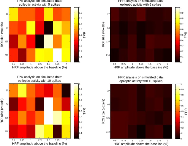
Fig. 1- Relative spatial and temporal sensitivities of different functional brain imaging methods. MEG: magnetoencephalography; sEEG: scalp electroencephalography; fMRI: functional magnetic resonance imaging; PET: positron emission tomography; SPECT: single photon emission computed tomography. Adapted from (Jezzard et al. 2001)... 2 Fig. 2- BOLD Signal Response to a brief stimulus. Adapted from (Jezzard 1999). ... 3 Fig. 3- Steps involved in the processing of fMRI data. Adapted from (Clare 1997). ... 4 Fig. 4- Results from an epileptic patient with unknown focus localization. a: activation map of peaks determined with TCA; b: histogram output from TCA; c: response of the voxel indicated by the arrow (dotted line) with modeled BOLD response time course (solid line). Adapted from (Morgan et al. 2004). ... 9 Fig. 5- Statistical maps from a subject with epilepsy obtained with models derived from TCA and from EEG. Adapted from (Hamandi et al. 2005). ... 10 Fig. 6- Graphical depiction of the TCA and 2dTCA algorithms showing how multiple reference time courses are created by the 2dTCA algorithm when multiple different voxel time courses are present in the data (Morgan et al. 2008). x represents the time point at which the voxel’s time series is maximum. y represents the time point at which occurs a significant signal increase on the time series. ... 12 Fig. 7- Depiction of the two regions in which the epileptic activity was simulated. A) 216 voxels cubic regions located at the left temporal lobe. B) 216 voxels cubic regions located at right frontal lobe. In each frame, A) and B), the top left, top right, and bottom left images represent a sagittal, coronal and transverse view, respectively. ... 13 Fig. 8- BOLD signal created by the convolution of the HRF with a spike train containing the timing of each event (Top) and its addition to the BOLD signal already presented in the real data (Bottom). ... 14 Fig. 9- Example of the three baselines (one corresponding to the mean of each cluster) estimated from k-means technique. The scale at the right represents the percentage signal change computed with the baseline corresponding to the mean of the middle cluster. ... 15 Fig. 10- Average sensitivity/specificity analysis for thresholds definition of candidate voxels selection step. Keeping the average sensitivity above 90 %, the best average specificity (red circle) was found for up and low boundaries of 3 and 0.5%, respectively, and a threshold of 2 standard deviations above the baseline with a TPR equal to 0.98 and a correspondent FPR equal to 0.59. The area under the curve is equal to 0.62. ... 16

(15)

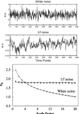
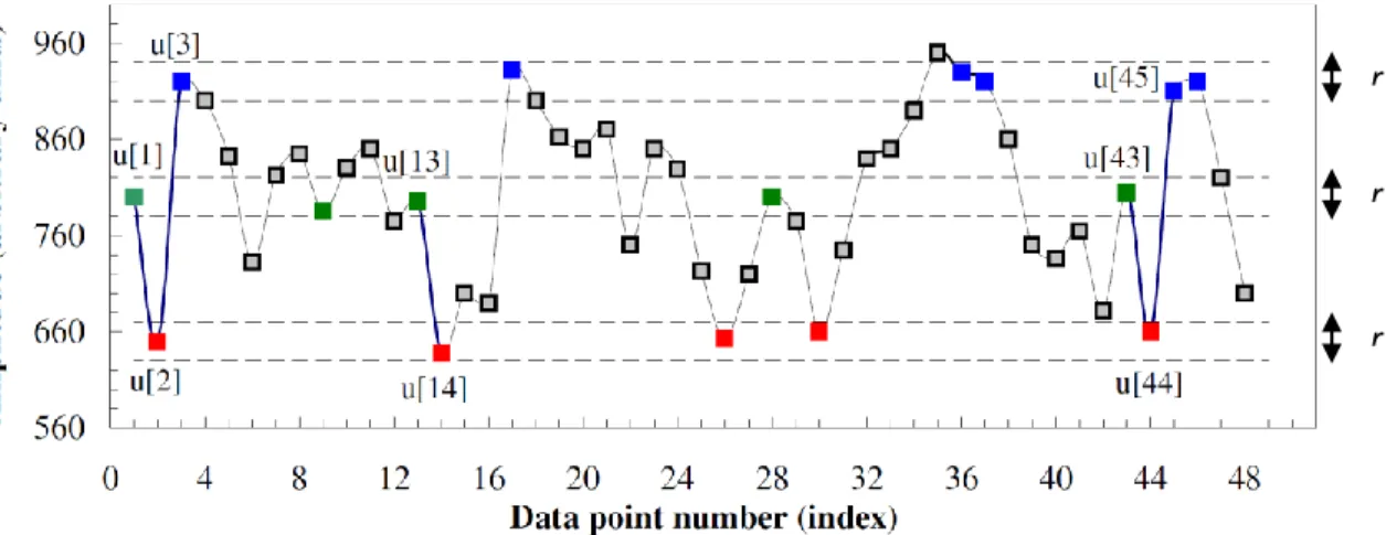
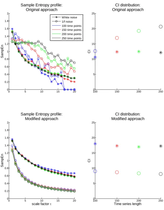
xii Fig. 11- Illustration of the second step of grouping RTCs. It is based on the percentage of shared activity between two RTCs. A: Temporal profile of two hypothetic RTCs. B: binary representation of each RTC spike above the mean, where the white color represents activations. ... 18 Fig. 12- Average sensitivity/#RTCs analysis for correlation coefficient (Top) and shared activity (Bottom) threshold definition of RTC grouping step. Optimal parameters for correlation coefficient and shared activity threshold were both defined as 0.7 with a correspondent average TPR and FPR and an average of RTCs number of 0.52, 0.0632 and 18.8 for the first threshold and 0.518, 0.0628 and 18.9 for the second threshold, respectively. ... 19 Fig. 13- TPR (left column)/FPR (right column) analysis on simulated data among ROIs size and HRF amplitude above the baseline. Top row: simulated epileptic activity with 5 spikes. Bottom row: simulated epileptic activity with 10 spikes. ... 20 Fig. 14- Schematic illustration of the coarse-graining procedure (Costa et al. 2005). ... 23 Fig. 15- Top: Simulated white and 1/f noises. Bottom: MSE analysis of simulated white and 1/f noise time series. Adapted from (Costa et al. 2005). ... 24 Fig. 16- Schematic illustration of the modified coarse-graining procedure where a moving average is applied to the original time-series for each scale factor. Adapted from (Costa et al. 2005). ... 26 Fig. 17- Illustration of sample entropy computation. In this example, the pattern length m and the tolerance r are 2 and 20, respectively. Dotted horizontal lines around data points u[1], u[2] and u[3] represent u[1] ± r, u[2] ± r, and u[3] ± r, respectively. All green, red, and blue, points represent data points that match the data point u[1], u[2], and u[3], respectively. Adapted from (Costa et al. 2005). ... 27 Fig. 18- Scoring classification for each possible pair of parameters (pattern length - m, tolerance - r) with a tested m = 2 (light blue) and 3 (dark blue) and r = 0.1 to 0.5 in steps of 0.05. Each bar represents the total score attributed to that case. The results showed that the optimal values for m and r are 3 and 0.4 times the standard deviation, respectively, with a total score of 67. 28 Fig. 19- Top: Sinusoidal time series with a frequency and sample frequency of 0.01 Hz and 0.5 Hz, respectively, and a length of 250 time points. Bottom: 1/f2 noise time series with a length of 250 time points. ... 30 Fig. 20- Sample entropy profile (computed with m=3 and r=0.4) over scale for original time series of white (asterisk) and 1/f (circle) noises of length 1000 time points using the original (blue) and the modified (red) MSE algorithm. ... 31 Fig. 21- Left: Sample entropy profile (computed with m=3 and r=0.4) over scale for original time series of white (asterisk) and 1/f (circle) noises with lengths in the range of 100 to 250 time points, in increments of 50, using the original (Top) and the modified (Bottom) MSE algorithm.

(16)

xiii Right: CI distribution in function of time series length correspondent to the sample entropy analysis presented at left. ... 32 Fig. 22- Left: Sample entropy profile (computed with m=3 and r=0.4) over scale for time series of white (in blue), 1/f (in red) and 1/f2_{(in green) noises, and sinusoidal signals of 0.01 Hz (in cyan)}

and 0.1 Hz (in black) with a length of 250 time points using the modified MSE algorithm. Right: Corresponding CI values for each signal type presented at left. CIWhite noise = 17.2; CI1/f noise = 8.1;

CI1/f2 noise = 3.8; CIsinusoid 0.01 Hz = 3.2; CIsinusoid 0.1 Hz = 0 ... 33

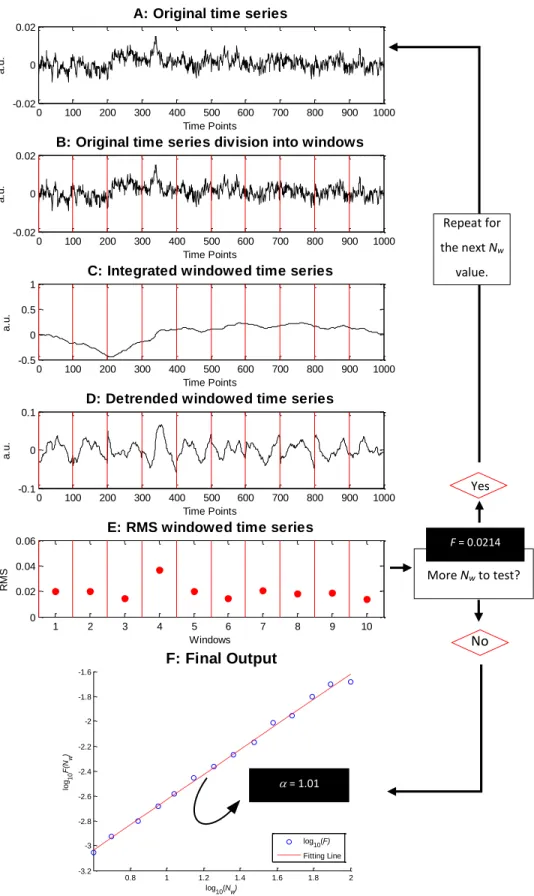
Fig. 23- Illustration of DFA algorithm steps. For this example a 1/f noise time series was created with a length of 1000 time points. The steps A to E represents the procedure for a window length, Nw, of 100 data points. F represents the final output when the previous steps were

repeated for all Nw values. : scaling exponent; F: RMS fluctuation. ... 39

Fig. 24- Scoring classification for each possible pair of parameters (maximum percentage - pmax,

overlap) with a tested range 50 % (dark blue), 40 % (light blue), 30 % (white), 20 % (gray), and 10 % (black) for pmax and 0 to 50 % in steps of 10 % for the overlap. Each bar represents the total

score attributed to that case. The results showed that the optimal values for pmax and overlap

are both 40 % with a total score of 117. ... 40 Fig. 25- Double logarithmic plot of fluctuations (computed with pmax and overlap equal to 40 %)

over window length for white (asterisk) and 1/f (circle) noise time series of length 1000 time points using the DFA algorithm. The fitting line for each fluctuations profile is represented at red for white and at blue for 1/f noises. ... 42 Fig. 26- Left:  value (computed with pmax and overlap equal to 40 %) for time series of white

(asterisk) and 1/f (circle) noise with lengths of the time series in the range of 100 to 250 time points, in increments of 50, using the DFA algorithm. Right: AI distribution in function of time series length correspondent to the  values presented at the left. ... 43 Fig. 27- Left: Double logarithmic plot of fluctuations (computed with pmax and overlap equal to

40 %) over window length for time series of white (in blue), 1/f (in red) and 1/f2_{(in green) noises,}

and sinusoidal signal of 0.01 Hz (in cyan) and 0.1 Hz (in black) with a length of 250 time points using DFA algorithm. Right: Corresponding  values for each signal type presented at left. White noise = 0.52; 1/f noise = 0.94; 1/f2 noise = 1.3; sinusoid 0.01 Hz = 1.6; sinusoid 0.1 Hz = 0.093. ... 43

Fig. 28- Influence of sample frequency and sinusoidal frequency (in Hz) on  value. ... 44 Fig. 29- Flowchart illustrating the pipeline analysis of real subject data, namely, epileptic patients’ dataset. : scaling exponent; AI: Anisotropy index; CI: Complex Index; DFA: Detrended Fluctuation Analysis; GLM: General Linear Model; FEWR: Family-Wise Error Rate; k: extended threshold; MSE: Multiscale Entropy; RTC: Reference Time Course; SPM: Statistical Parametric

(17)

xiv Map. Circles on CI/ distribution: blue: white noise; red: 1/f noise; green: 1/f2_{noise; cyan:}

sinusoid of 0.01 Hz; black: sinusoid of 0.1 Hz. ... 49 Fig. 30- Histogram showing the distribution of the number of voxels with a given value of the transient spike selection limit [2 standard deviations (std) above the baseline] for patient 1. Red dashed lines represents the lower and upper boundaries of allowed signal change (see Chapter 2: 2.2.2 Algorithm implementation – Candidate voxels selection). ... 53 Fig. 31- Results for patient 1. Left: bi-dimensional histogram with the counting of transient spikes over the time. Each column represents a preliminary RTC. Right diagonal profile representing the number of voxels which maximum occurs in each time point. ... 54 Fig. 32- Activation maps from RTC_1, RTC_5, RTC_7 and RTC_15 obtained using 2dTCA (FEWR correction, p-value<0.05, k-threshold=27 voxels) and corresponding RTCs’ temporal profiles. Results for patient 1. S: superior; I: inferior; A: anterior; P: posterior; R: right; L: left. ... 55 Fig. 33- Correlation matrix between ipsi and contralteral clusters of all RTCs that produced SPMs with significant activation. Results for patient 1. Each label on the left of the matrix as the form of ‘Idx: RTC#_size’ or ‘Idx: RTC#_size_c’, where Idx represents the index of the label, # the number of the RTC that produced the SPM, size stands for the size of the cluster being analyzed, and c means contralateral cluster. On the bottom of the matrix are the labels with the same indexes as those presented on the left. ... 56 Fig. 34- Distribution of the mean CI and  across each cluster of RTC 5 and the CI and  for the ipsi and lateral cluster of RTC 7. At blue are the mean parameters for ipsilateral clusters and at red are the mean parameters for contralateral clusters. Results for patient 1. ... 56 Fig. 35- Anisotropy analysis of each cluster considered for further analysis. At green is the target region. Each red point is labeled in the following way: ‘Number of the RTC’-‘Size of the RTC’. Results for patient 1. ... 57 Fig. 36- CI/ distribution of each cluster considered for further analysis. Each red point is labeled in the following way: ‘Number of the RTC’-‘Size of the RTC’. Results for patient 1. ... 58 Fig. 37- Functional connectivity maps of RTC5_30 (the potential epileptogenic focus chosen by complexity analysis) in z-score and thresholded at ±0.51. Results for patient 1. L: left; R: right. ... 58 Fig. 38- Histogram showing the distribution of the number of voxels with a given value of the transient spike selection limit [2 standard deviations (std) above the baseline] for patient 2. Red dashed lines represents the lower and upper boundaries of allowed signal change (see Chapter 2: 2.2.2 Algorithm implementation – Candidate voxels selection). ... 59

(18)

xv Fig. 39- Results for patient 2. Left: bi-dimensional histogram with the counting of transient spikes over the time. Each column represents a preliminary RTC. Right diagonal profile representing the number of voxels which maximum occurs in each time point. ... 59 Fig. 40- Activation maps from RTC_1, RTC_2, RTC_3, RTC_5, RTC_10, and RTC_14 obtained using 2dTCA (FEWR correction, p-value<0.05, k-threshold=27 voxels) and corresponding RTCs’ temporal profiles. Results for patient 2. S: superior; I: inferior; A: anterior; P: posterior; R: right; L: left. ... 61 Fig. 41- Correlation matrix between ipsi and contralteral clusters of all RTCs that produced SPM with significant activation. Results for patient 2. Each label on the left of the matrix as the form of ‘Idx: RTC#_size’ or ‘Idx: RTC#_size_c’, where Idx represents the index of the label, # the number of the RTC that produced the SPM, size stands for the size of the cluster being analyzed, and c means contralateral cluster. On the bottom of the matrix are the labels with the same indexes as those presented on the left. ... 62 Fig. 42- Distribution of the mean CI and  across each cluster of RTC_3, RTC_5, RTC_10, and RTC_14 and the CI and for the ipsi and contralateral cluster of RTC_2. At blue are the mean parameters for ipsilateral clusters and at red are the mean parameters for contralateral clusters. Results for patient 2. ... 63 Fig. 43- Anisotropy analysis of each cluster considered for further analysis. At green is the target region. Each red point is labeled in the following way: ‘Number of the RTC’-‘Size of the RTC’. Results for patient 2. ... 63 Fig. 44- CI/ distribution of each cluster considered for further analysis. Each red point is labeled in the following way: ‘Number of the RTC’-‘Size of the RTC’. Results for patient 2. ... 64 Fig. 45- Functional connectivity maps of RTC10_92 (the potential epileptogenic focus chosen by complexity analysis) in z-score and thresholded at ±0.4. Results for patient 2. L: left; R: right. 65 Fig. 46- Histogram showing the distribution of the number of voxels with a given value of the transient spike selection limit [2 standard deviations (std) above the baseline] for patient 3. Red dashed lines represents the lower and upper boundaries of allowed signal change (see Chapter 2: 2.2.2 Algorithm implementation – Candidate voxels selection). ... 65 Fig. 47- Results for patient 3. Left: bi-dimensional histogram with the counting of transient spikes over the time. Each column represents a preliminary RTC. Right diagonal profile representing the number of voxels which maximum occurs in each time point. ... 66 Fig. 48- Activation maps from RTC_1, RTC_3, RTC_4 and RTC_11 obtained using 2dTCA (FEWR correction, p-value<0.05, k-threshold=27 voxels) and corresponding RTCs’ temporal profiles. Results for patient 3. S: superior; I: inferior; A: anterior; P: posterior; R: right; L: left. ... 67

(19)

xvi Fig. 49- Correlation matrix between ipsi and contralteral clusters of all RTCs that produced SPM with significant activation. Results for patient 3. Each label on the left of the matrix as the form of ‘Idx: RTC#_size’ or ‘Idx: RTC#_size_c’, where Idx represents the index of the label, # the number of the RTC that produced the SPM, size stands for the size of the cluster being analyzed, and c means contralateral cluster. On the bottom of the matrix are the labels with the same indexes as those presented on the left. ... 68 Fig. 50- Distribution of the mean CI and  across each cluster of RTCs 1, 3, 4, and 11. At blue are the mean parameters for ipsilateral clusters and at red are the mean parameters for contralateral clusters. Results for patient 3. ... 69 Fig. 51- Anisotropy analysis of each cluster considered for further analysis. At green is the target region. Each red point is labeled in the following way: ‘Number of the RTC’-‘Size of the RTC’. Results for patient 3. ... 69 Fig. 52- CI/ distribution of each cluster considered for further analysis. Each red point is labeled in the following way: ‘Number of the RTC’-‘Size of the RTC’. Result for patient 3. ... 70 Fig. 53- Functional connectivity maps of RTC11_39 (the potential epileptogenic focus chosen by complexity analysis) and RTC4_55 (the cluster that best described the anatomical brain region with lesion) in z-score and thresholded at ±0.36 and ±0.46, respectively. Results for patient 3. L: left; R: right... 70

(20)

xvii

LIST OF TABLES

Table 1- Epileptic patients sample characterization: gender, age, type of epilepsy, and localization of its epileptogenic focus. F: female; M: male; TLE: temporal lobe epilepsy; FCDE:

focal cortical dysplasia epilepsy. ... 48

Table 2- Number and size of the clusters presented in each SPM of patient 1. ... 54

Table 3- Number and size of the clusters presented in each SPM of patient23. ... 60

(21)

xviii

LIST OF ACRONYMS

2dTCA Two-dimensional Temporal Clustering Analysis

  Scaling Exponent

AI Anisotropy Index

BOLD Blood Oxygen Level Dependent

CI Complexity Index

dHb Deoxyhemoglobin

EEG Electroencephalography EPI Echo Planar Imaging

FDG Fluorodeoxyglucose

fMRI Functional Magnetic Resonance Imaging FWER Family-Wise Error Rate

DFA Detrended Fluctuation Analysis DMN Default Mode Network

GLM General Linear Model

HRF Hemodynamic Response Function ICA Independent Component Analysis iEEG Intracranial Electroencephalography LRTC Long-Range Temporal Correlations

MEG Magnetocencephalography

MSE Multiscale Entropy Analysis

oHb Oxyhemoglobin

PET Positron Emission Tomography

RMS Root-Mean-Square

ROI Region-of-Interest RTC Reference Time Course

(22)

xix sEEG Scalp Electroencephalography

SPM Statistical Parametric Map SNR Signal-to-Noise Ratio TCA Temporal Clustering Analysis

(23)

1

CHAPTER 1. INTRODUCTION AND OBJECTIVES

Epilepsy is one of the most important chronic neurological disorders worldwide affecting more than 50 million people of all ages. Although 70% of the cases are treatable with anti-epileptic drugs and less than 10% with surgical therapy, the remaining 20% can’t control their seizures. This neurological disorder brings an important impact on epileptic patients concerning discrimination, social stigma, and higher national healthcare costs. People with epilepsy can be targets of prejudice and the stigma of the disorder can discourage people from seeking treatment for symptoms and becoming identified with the disorder (WHO 2012).

An epileptic seizure can be defined as a “transient occurrence of signs and/or symptoms due to abnormal excessive or synchronous neuronal activity in the brain” (Fisher et al. 2005). These brief electrical disturbances can have effects on sensory, motor, and autonomic functions, provoke changes in awareness or behavior, loss of consciousness, and convulsions. Uncontrolled epilepsy can also lead to depression, anxiety, and loss of cognitive function (Avanzini et al. 2013).

The epileptogenic zone or focus is a theoretical concept corresponding to the brain volume that needs to be removed to render the patients seizure-free, i.e., it describes the abnormal cortex responsible for the generation of epileptic seizures. Thus, the cessation of seizures is accomplished with the complete resection of this area (Hamandi et al. 2005). This focus is characterized by two types of electrical activity, ictal which means during seizure, and interictal, which mean between seizures. The last one is normally more brief in time and is periodic (Ko et al. 2014).

Hereupon, epileptogenic focus identification is important to epilepsy diagnostic and seizure control. The present methods for this purpose are based on Positron Emission Tomography (PET) and Single Photon Emission Computed Tomography (SPECT) (Mountz 2007; Kim & Mountz 2011), Magnetoencephalography (MEG) (Foley et al. 2014), Electroencephalography (EEG) alone (Hassanpour et al. 2004; Leal et al. 2007; Leal et al. 2008) and EEG/functional Magnetic Resonance Imaging (fMRI) analysis (Leal et al. 2006; Leite et al. 2013; Wang et al. 2012; Hamandi et al. 2005; Thornton et al. 2010). There’s a tradeoff in terms of time and spatial resolutions for all these techniques (Fig. 1). The first technique is a direct measure of the Fluorodeoxyglucose (FDG) uptake in the brain based on the hypotheses that the cortical blood flow increases in the area of seizure

(24)

2 discharge (Mountz 2007). The second

one works is a similar way, but with a different radiotracer (Tc-99m) (Kim & Mountz 2011). The main limitation of using PET and SPECT to localize the epileptogenic zone relies on specificity of abnormalities due to its limited spatial resolution and poor temporal resolution (Morgan et al. 2004; Clare 1997). Furthermore, the need for a radiotracer is also a drawback, making this technique more invasive.

The third and fourth techniques used to localize ictal and interictal electrical activity are MEG and EEG. There are two main modes of using the latter modality, scalp EEG (sEEG) and intracranial EEG (iEEG). Both of these modalities have high temporal resolution, allowing the detection of brief spikes of electric activity, such as interictal activity. However, when regarding the needs of abnormalities’ specificity for presurgical assessment, the spatial resolution of sEEG and MEG is poor. In order to improve the resolution of sEEG a high-density of electrodes is needed (Leal et al. 2007; Leal et al. 2008). This issue can be overcome by iEEG, as the electrical signal is recorded directly from cortical tissue. The major drawback of this last modality relies on the fact that it’s extremely invasive. Lastly, simultaneous EEG-fMRI is an emergent technique which combines the best of two modalities, high temporal resolution from EEG and high spatial resolution from fMRI. The strategy followed in this case is to continuously sample the interictal and ictal events while measuring the BOLD signal simultaneously with EEG. This is somewhat cumbersome as it requires a very specific and delicate setup, particularly for acceptable recording of the EEG. Otherwise it will bring several kinds of noise problems, including movements artifacts (Wang et al. 2012), compromising the feasibility of EEG-fMRI studies. Another shortcoming associated with this technique, and with EEG alone, is that they aren’t sensitive to interictal epileptiform activity in deep structures making this technique useful only in patients with frequent interictal events recorded from the sEEG (Morgan et al. 2004; Lopes et al. 2012). To overcome some of the limitations described above and find a more suitable solution to localize a seizure onset, efforts are being taken to develop new processing methods using fMRI Fig. 1- Relative spatial and temporal sensitivities of different functional

brain imaging methods. MEG: magnetoencephalography; sEEG: scalp electroencephalography; fMRI: functional magnetic resonance imaging; PET: positron emission tomography; SPECT: single photon emission computed tomography. Adapted from (Jezzard et al. 2001).

SPECT MEG/

(25)

3 technique only (Yee & Gao 2002; Morgan et al. 2004; Hamandi et al. 2005; Morgan et al. 2008; Morgan et al. 2010).

Another approach to epilepsy diagnosis and characterization of epileptic signals behavior has been recently taken on the complexity field. Some authors have been hypothesized that epileptogenic brain tissue has a different complexity than healthy brain tissue (Parish et al. 2004; Monto et al. 2007; Protzner et al. 2010). A complete characterization of this complexity could lead to a definition of a physiological biomarker applicable to epilepsy, namely for diagnostic and monitoring of its treatment. For that purpose two main approaches can be used: a disorder level based (Ouyang et al. 2009; Protzner et al. 2010) or a fractal properties based (Parish et al. 2004; Monto et al. 2007) methods. In both of them it is expected that in the epileptogenic focus the complexity is lower because of its intrinsic periodic interictal electric activity.

This thesis project will focus on the epileptic focus localization through fMRI BOLD signals and then on the complexity analysis of its time series. Therefore, in the next section the concepts inherent to this work will be described.

1.1. BOLD signal origin and fMRI analysis

Functional magnetic resonance imaging (fMRI) is a powerful non-invasive tool that allows the study of the functional responses of the brain in a quantitative way. One advantage of using fMRI is the identification of brain activity due to a stimulus with a high spatial resolution (Jezzard et al. 2001). This technique is based on the

hemodynamic response function (HRF) of the brain, which arises when a given stimulus is applied. The HRF is a transfer function of the neurovascular coupling characteristic of brain activation. When a stimulus acts on a particular region of the brain evokes, in that area, a change in blood flow. This facilitates

Fig. 2- BOLD Signal Response to a brief stimulus. Adapted from (Jezzard

1999).

B

C A

(26)

4 glucose oxidation by providing more oxygen molecules. If there is an increased consumption of oxygen, there’ll be an increased concentration of deoxyhemoglobin (dHb), a paramagnetic oxygen binding molecule. Oxyhemoglobin (oHb), on the other hand, is a diamagnetic molecule with a magnetic susceptibility smaller than that of dHB (Clare 1997).

Therefore, a change in hemoglobin oxygenation leads to changes in the local distortions of a magnetic field applied, generating local field gradients and local changes of T2* in tissue the blood vessels. The measure of the T2* originate the BOLD signals (Jezzard et al. 2001), see Fig. 2. The brain hemodynamic response can be summarized in the following steps. When a brief stimulus acts, there’s an initial decrease of BOLD signal due to increase of oxygen consumption (Fig. 2A). Then, the increased blood flow decreases the dHb concentration increasing the BOLD signal (Fig. 2B). Finally, a delay of the return to the initial blood volume level provokes a decrease of oHb, and a consequently increase of dHb reducing temporally the BOLD signal intensity (Fig. 2C).

The output of fMRI is a set of volumes comprising the scans of the brain at successive times, usually named raw data. Each volume is divided in resolution dependent number of small elements, named voxels, in which the information of the correspondent brain region is stored. One of the goals of acquiring fMRI data is to perform a robust, sensitive, and valid analysis to detect brain regions that show increased signal intensity at the stimulus time. In other words, the aim of fMRI analysis is to identify which voxels have their signal significantly greater than the noise level (Clare 1997; Jezzard et al. 2001). A typical pipeline analysis, schematically represented in Fig. 3, includes a first step of raw data pre-processing that usually includes, correction to time effects and

to subject movement during the experiment, and data spatial smoothing to improve the signal to noise ratio. Additional steps, such as, data detrending, filtering and regressing out of nuisance covariates are often taken. The aim of this pre-process is to improve the detection of activation events. Then, a statistical analysis is performed to detect which voxels shows a response to the assessed stimulus. This step usually involves a model estimation, through a general linear model (GLM) based on convolution between the HRF and the stimulus temporal profile. Finally, in order to display the activation images, statistical confidence must be given to the results by inferring about

Raw Data

Pre-processing

Statistical analysis

Inference and Presentation

Fig. 3- Steps involved in the processing of

(27)

5 probability values. See Appendix A for more information about statistical analysis, inference and statistical maps presentation in fMRI.

The assessment of a stimulus via a pipeline analysis as described above can be one of two types. The first one comprises a stimulus that has typically few time points of duration, and its analysis is usually named a block-related one. The second one, a transient stimulus with a short duration is used, whereby its analysis is named an event-related one (Josephs et al. 1997). In epilepsy, once the stimulus is usually a transient spike corresponding to interictal electric activity, the analysis described in the above pipeline of event-related type.

Since no technique is free of shortcomings this one has several limitations too. One of them concerns the temporal resolution, which is limited by the profile of the hemodynamic response, and low signal-to-noise ratio (SNR) and contrast-to-noise ratio (CNR), leading to high variance in the results. One way to overcome this last limitation is to repeat the stimuli more than once, decreasing variance in results (Jezzard et al. 2001). However, this is difficult to apply in epilepsy since the timing of the stimulus, interictal or ictal seizure activity, is random and uncontrollable (Morgan et al. 2007).

1.2. Epileptogenic focus localization

As explained before, the timing of ictal and interictal activity in epilepsy is unknown and unpredictable. Therefore, an analysis based on models isn’t suitable to localizing the epileptogenic focus, since no assumptions about temporal profile of the stimuli can be made. Data-driven techniques have been developed to deal with such cases as they are model-free. Some examples of such methods are the following: principal component analysis (Sugiura et al. 2004; You et al. 2011), independent component analysis (ICA) (Rodionov et al. 2007), hierarchical clustering (Cordes et al. 2002; Keogh et al. 2005), and fuzzy clustering (Somorjai & Jarmasz 2003; Wahlberg & Lantz 2000). When applied to fMRI datasets these methods result in a large number of components, which are hard to classify without spatial and temporal information (De Martino et al. 2007; Rodionov et al. 2007).

Another data-driven method developed in the past years is temporal clustering analysis (TCA) (Yee & Gao 2002; Gao & Yee 2003; Morgan et al. 2004; Hamandi et al. 2005). This is a one-dimensional algorithm that groups together time series to one single cluster with the same temporal profile based on a given criteria. This criterial could be, for example, the same maximum signal magnitude

(28)

6 timing or the same first signal magnitude increase, to one single cluster. A modification of the original TCA to a bi-dimensional method, two-dimensional temporal clustering analysis (2dTCA) (Morgan et al. 2007; Morgan et al. 2008), detects different BOLD responses, assumed to be from different sources. It allows the detection of more than one single cluster. Once obtained the temporal profile of the cluster, it is possible to perform an event-related fMRI analysis.

In Morgan’s work (Morgan et al. 2007; Victoria L Morgan et al. 2008; Morgan et al. 2010) the application of 2dTCA to epileptogenic focus localization is based on the hypothesis that interictal epileptic activity provokes a transient BOLD spike with a rate slower than that of BOLD images acquisition. This hypothesis was based on preview results of EEG-fMRI studies applied to temporal lobe epilepsy (Salek-Haddadi et al. 2006; Kobayashi et al. 2005; Federico et al. 2005; Bagshaw et al. 2004). The main results of these works showed that interictal activity detected by EEG is associated with a BOLD signal change.

1.3. Complexity analysis

The human brain has an inherent high complexity arising from the interaction of thousands of neuronal networks that operates over a wide range of temporal and spatial scales (Hutchison et al. 2013). This enables the brain to adapt to the constantly changing environment and to perform mental functions. In pathologic brains this capacity of adaptation is often impaired, leading to ordered or random patterns of behavior. In case of epilepsy, the study of such complexity could help to understand how an epileptic brain functions.

To assess brain complexity we can only observe the macroscopic output of brain function, such as via EEG and fMRI, where a signal change represents a response from millions of neurons, thus creating the need for robust methods to evaluate the complexity of signal from such techniques. These methods are usually based on one of two approaches: disorder level based or a fractal properties based.

The first one comprises methods that are entropy-based, by quantifying the regularity or orderliness of a time series (Pincus 1991; Kurths et al. 1996; Andino et al. 2000; Richman & Moorman 2000). Entropy can be conceptualized has a measure of the degree of disorder of a given system and increases with the degree of irregularity, reaching its maximum in completely random systems, such as uncorrelated or white noise, and its minimum in completely ordered systems, such as a single

(29)

7 frequency sinusoid. Physiologic outputs usually exhibits a higher degree of entropy under healthy conditions than in a pathological state, as they’re characterized by a sustained breakdown of long-range correlations and loss of information (Goldberger et al. 2002). However, an increase in the entropy may not always be associated with an increase in dynamical complexity (Costa et al. 2002). One method that has been developed and improved in the past years and has been shown to effectively quantify the complex dynamics of biological signals is the multiscale entropy (MSE) (Costa et al. 2002). It is based on measuring the entropy over multiple time scales inherent in a time series. The second approach on brain complexity assessment relies on the evaluation of long-range temporal correlations (LRTC), which reflect the self-affinity of a given signal. The majority of quantifications methods such as spectral analysis and Hurst analysis (Peng et al. 1995) for the LRTC study are invalid to evaluate biological signals because, as they are complex and show fractal properties, their stationarity are not guarantee. Thus, a method capable of detecting the LRTC was developed in the past years to overcame the nonstationary problem of biological signals, named detrended fluctuation analysis (DFA) (Peng et al. 1994).

1.4. Thesis hypotheses and goals

This master thesis project is based on the hypotheses that the epileptogenic focus shows a BOLD signal with a distinct temporal profile from the remaining brain parenchyma, either during ictal and interictal activity (Morgan et al. 2007; Victoria L Morgan et al. 2008; Morgan et al. 2010). Particularly, it is known that the interictal epileptic activity provokes a transient BOLD spike with a rate slower than that of BOLD images acquisition (Salek-Haddadi et al. 2006; Kobayashi et al. 2005; Federico et al. 2005; Bagshaw et al. 2004). This makes possible the application of a method for the localization of the epileptogenic focus, the 2dTCA.

Furthermore, it is well-known, from epileptic EEG signal studies, the periodic behavior of epileptic activity of epileptogenic brain regions (Parish et al. 2004; Monto et al. 2007; Protzner et al. 2010). Indeed, in these EEG studies it was shown that the epileptogenic focus EEG signal shows lower complexity than healthy parenchyma. However, there are no studies showing the same results with epileptic BOLD signals. Therefore, for the purpose of this thesis project it is hypothesized that the epileptogenic focus BOLD signals shows lower complexity than healthy parenchyma. Also, this complexity can be assessed by methods like MSE and DFA.

(30)

8 Summarizing, the innovation of this work is to explore the complexity properties of epileptic BOLD signals through the application of an algorithm that localizes the epileptogenic focus and extracts its BOLD signal. The main aim is to provide a definition of a biomarker for epileptic tissue identification in order to help on the diagnostic, monitoring and treatment of epilepsy.

Hereupon, this thesis project have three main goals. First, the algorithms referred above, the 2dTCA, the MSE, and the DFA, will be implemented in Matlab®1_{language using the commercial software}

package Matlab® R2014a. All of these methods will be optimized for BOLD signals analysis using simulated data. Second, a study with a sample of epileptic patients will be carried out by first localizing potential epileptogenic foci with 2dTCA and analyzing complexity of its BOLD signal in order to compare with those of healthy brain parenchyma. Third, based on the hypotheses stated above, the most likely epileptogenic focus will be chosen.

(31)

9

CHAPTER 2. BI-DIMENSIONAL TEMPORAL CLUSTERING ANALYSIS

2.1. Introduction

TCA was firstly introduced by Liu and colleagues with a pioneer work where this method was used to study the temporal response of the brain after eating (Liu et al. 2000). The problem addressed by this approach was the fact that there’s no model assumption that can be taken to estimate which brain regions will be activated after eating, once the activation timing is unknown. This algorithm searches for the maximal response in each voxel’s time series converting a four-dimensional data, characterized in terms of space and time, into a simple relationship between the number of voxels reaching maximum signals and the time, named histogram. A concept of brain parcellation that accounts for timing and connectivity was accomplished for the first time with the results of this work.

In order to improve the brain activations timing detection Yee and Gao modified the sensitivity of TCA algorithm basing the method on the integrated signal intensity of a temporal cluster at each time point (Yee & Gao 2002; Gao & Yee 2003) rather than only on the size of a temporal cluster (Liu et al. 2000). In other words, in the modified algorithm a condition is superimposed limiting the maximum signal change allowed to be clustered. The results of Yee and Gao work show that, despite the fact that the modified TCA is more sensitive than the original one, neither of them could detect

Fig. 4- Results from an epileptic patient with unknown focus localization. a:

activation map of peaks determined with TCA; b: histogram output from TCA;

c: response of the voxel indicated by the arrow (dotted line) with modeled

(32)

10 peaks smaller than the noise level. This opened a window to novel problems, like time shift and movement artifacts, that needed to be addressed before the TCA application.

The application of TCA to epileptogenic focus localization was first addressed by Morgan and colleagues in (Morgan et al. 2004) under the hypothesis that the timing of interictal activity could be determined using TCA on resting fMRI data. Then, activation maps created by event-related fMRI analysis using the discovered discharges timings could be determined to show which brain regions are presumably part of the epileptogenic focus. The result from an epileptic patient with unknown focus localization is shown in Fig. 4. It shows the histogram output from the TCA (Fig. 4b), the results of statistical analysis (Fig. 4a), and fitted and adjusted responses of one voxel pertaining to the found cluster (Fig. 4c). The fact that the TCA defines one single histogram, i.e., one single cluster, implies that voxels spatially distant may be grouped together (as seen in Fig. 4). Whether this detected cluster temporal profile is a representation of the epileptogenic focus or instead a mixture of sources can’t be assessed and, therefore, the effectiveness of TCA can’t be assessed as well.

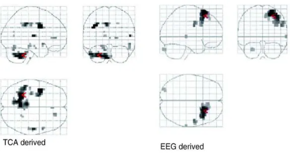
Fig. 5- Statistical maps from a subject with epilepsy obtained with models derived from TCA and from EEG. Adapted from

(Hamandi et al. 2005).

Hamandi and colleagues assessed the TCA performance by implementing and evaluating it, as described in (Morgan et al. 2004), using fMRI data acquired with simultaneous EEG in patients with clearly defined focal epilepsy and frequent interictal discharges (Hamandi et al. 2005). They demonstrated that the temporal clusters found were closely correlated with motion events, and not interictal epileptic activity, refuting the validity of using these as onsets in statistical analysis. In order to illustrate this issue, there’s a resultant statistical map from an epileptic patient is present

(33)

11 in Fig. 5. It represents the activated brain region found with models in which the onsets were derived either from TCA and EEG. As it can be seen those regions does not match with each other, contrary as expected, suggesting that there may be a confounding with motion events when performing TCA. Hamandi et al. work brought new insights about the limitations of using TCA applied to epilepsy, suggesting that in order to improve this methodology there is the need to primarily separate the noise from the stimuli source and then compare the performance of TCA with other method such as ICA, for example.

Morgan and colleagues posterior work (Morgan et al. 2007; Morgan et al. 2008) brought a new approach to this area by modifying the TCA methodology and overcoming some of the shortcomings described above. They developed a two-dimensional TCA technique addressing the problem of motion and physiological noise by detecting and sorting out separate BOLD responses assumed to be from different sources. This was based on the assumption that BOLD signal changes due to spontaneous interictal activity may be relatively small compared to those of noise, motion, and other activity and are expected to be only slightly slower than the rate of image acquisition (Morgan et al. 2008). Furthermore, as the shape of this BOLD signal response is well known it allows the application of the 2dTCA.

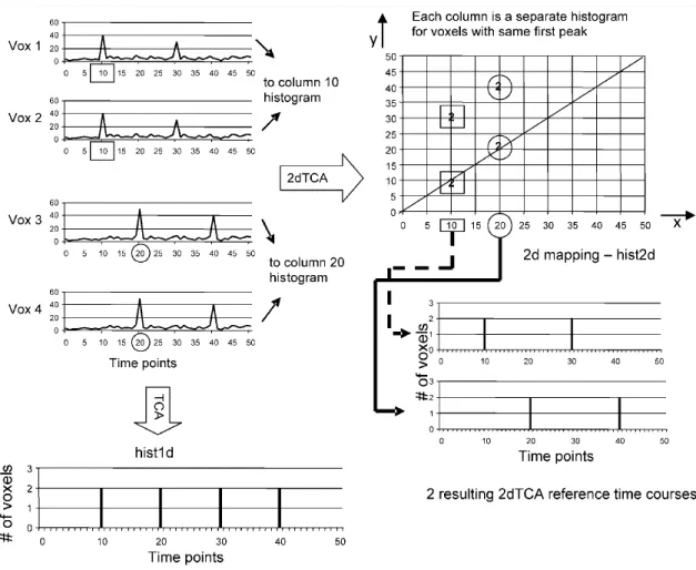
Briefly, in Fig. 6 is depicted a graphical representation of how 2dTCA works and a comparison with TCA. The 2dTCA algorithm will construct a bi-dimensional histogram where columns represent temporal clusters with different temporal profiles. The criterion of grouping time series to different clusters is based on the first time point at which the first signal increase occur, instead of grouping with maximum signal criteria (Liu et al. 2000; Yee & Gao 2002; Gao & Yee 2003; Morgan et al. 2004; Hamandi et al. 2005). This assumes that different sources of activation will not have overlapping timing of BOLD response at the beginning of the time series, which is not proven to be in that way. Supposing that in a functional dataset there are four voxels’ time series with different temporal profiles (Vox 1 to 4 in Fig. 6), using 2dTCA Vox 1 and 2 were grouped together in the same histogram column, representing a reference time course of one cluster. On the other hand Vox 3 and 4 will be are grouped together in another column, representing another and independent reference time course of a different cluster. If, for example, one group of voxels represent an epileptogenic focus and another a noising source, such as movement, this algorithm could rule out the latter by sorting different sources in different clusters. If a TCA approach were taken, all the voxel’s time courses would be grouped together leading to the identification of brain regions that aren’t related to epileptogenic tissue, similar to what was described in (Hamandi et al. 2005), see Fig. 5.

(34)

12 Fig. 6- Graphical depiction of the TCA and 2dTCA algorithms showing how multiple reference time courses are created by

the 2dTCA algorithm when multiple different voxel time courses are present in the data (Morgan et al. 2008). x represents the time point at which the voxel’s time series is maximum. y represents the time point at which occurs a significant signal increase on the time series.

In Morgan and colleagues’ work (Victoria L Morgan et al. 2008), the performance of 2dTCA was assessed, in terms of specificity and sensitivity, by comparing it with the performance of TCA and ICA applied to the same simulated data, where a well-known activations were defined (Morgan et al. 2008). The results showed that 2dTCA algorithm can detect more than one independent reference time course, or equivalently more than one temporal cluster, more effectively than TCA, but slightly less effectively than ICA. However, they argued that as the 2dTCA algorithm will cluster only transient spikes, while decreasing sensitivity to signals of other temporal characteristics, the large number of components determined with ICA would make it difficult to determine the components of interest in vivo when the activation regions are not known. This confirms the advantage of using the 2dTCA as a data-driven for identifying the epileptogenic focus.

x y

(35)

13 As a final remark about the application of 2dTCA on healthy subjects and epileptic patients, more recent work have demonstrated that this algorithm can also be used to detects clusters associated with the default-mode network (DMN) (Morgan et al. 2007; Morgan et al. 2008; Morgan et al. 2010; Pizarro et al. 2012) in healthy (Cauda et al. 2010; Fox et al. 2005)and epileptic subjects and with specific regions, such as the visual, auditory, and motor cortices, through external stimuli with known timing (Morgan & Gore 2009).

2.2. Materials and Methods

2.2.1. Simulated Dataset Characterization

Fig. 7- Depiction of the two regions in which the epileptic activity was simulated. A) 216 voxels cubic regions located at

the left temporal lobe. B) 216 voxels cubic regions located at right frontal lobe. In each frame, A) and B), the top left, top right, and bottom left images represent a sagittal, coronal and transverse view, respectively.

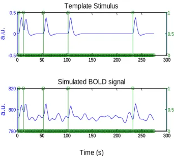
A simulated dataset was created, according to the pipeline presented in (Khatamian et al. 2011), from a preprocessed rest fMRI healthy subject scan (see Appendix B for more details of this subject data acquisition) by adding simulated BOLD signals in order to create simulated epileptic activity. For this purpose two regions of interest (ROI) were defined (see Fig. 7), one in the left temporal lobe (LTL) and the other in the right frontal lobe (RFL), to which simulated epileptic activity was added. BOLD signals representing this type of activity were created by convolving the HRF with a spike train containing the timing of each event (see Fig. 8) and added to the BOLD signal already presented in each ROI. The final goal was to obtain simulated data with all combinations of the following characteristics: 5 and 10 spikes randomly distributed in time, correspondent to LTL and RFL ROIs, respectively; simulated activation amplitudes of 0.5 to 2% in increments of 0.25%; and ROI’s size of 27, 64, 125, and 216 voxels. Within a ROI the activation frequency and amplitude is homogenous. Each simulation was repeated two times resulting in a total of 56 simulated datasets.

S P M m ip [-58. 5323, -28. 805, 8. 09453] < < < 0 1 2 3 x 10-3 S P M m ip [-58. 5323, -28. 805, 8. 09453] < < < 0 1 2 3 x 10-3 S P M m ip [10. 806, 57. 6349, 9] < < < 0 1 2 3 x 10-3 S P Mm ip [10. 806, 57. 6349, 9] < < < 0 1 2 3 x 10-3 A B

(36)

14 Fig. 8- BOLD signal created by the convolution of the HRF with a spike train containing the timing of each event (Top) and

its addition to the BOLD signal already presented in the real data (Bottom).

2.2.2. Algorithm implementation

The 2dTCA algorithm implemented in this thesis project is based mainly on (Morgan et al., 2008) work with some modified steps based on (Khatamian et al. 2011) and another additional original steps.

fMRI Data pre-processing

Concerning fMRI data, some pre-processing steps are expected before the beginning of the 2dTCA algorithm itself. Namely, slice timing correction for effects due to interleaved acquisition, realignment for correction of motion effects, spatial smoothing, detrending (an additional step not performed in (Morgan et al. 2008; Khatamian et al. 2011)), and temporal filtering. The type of filter used in this last step was a bandpass filter containing the frequencies expected in BOLD response (Glover 1999), instead of a 3-point averaging filter used in (Morgan et al. 2008).

Data transformation

Each functional data series was formatted into M one-dimensional arrays corresponding to the M analyzed voxels of the dataset. In other words, each array contained the voxel’s time series with N time points, given by the number of volumes of each raw data. The next steps were performed on this data. 0 50 100 150 200 250 300 -0.5 0 0.5 a .u . Template Stimulus 0 50 100 150 200 250 3000 0.5 1 0 50 100 150 200 250 300 780 800 820 a .u .

Simulated BOLD signal

0 50 100 150 200 250 3000 0.5 1 0 50 100 150 200 250 300 -0.5 0 0.5 a .u . Template Stimulus 0 50 100 150 200 250 3000 0.5 1 0 50 100 150 200 250 300 780 800 820 a .u .

0 50 100 150 200 250 3000 0.5 1 0 50 100 150 200 250 300 -2 0 2 Time (s) % c h a n g

(37)

15

Baseline definition and percent change computation

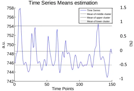
A definition of the baseline value as the average of the first 5 time points of the voxel’s time course as in (Morgan et al. 2008), implies an assumption that the subject is at baseline during that time, which may not be true. Therefore, a k-means technique was used such that each voxel’s time series was separated into three clusters: one with high values, another with low values, and the last one with the remaining middle values, see Fig. 9 . This differs from the two clusters used in (Khatamian et al. 2011) whereas it was assumed that the BOLD response can represent an activation, an increase in amplitude, or a deactivation, a decrease in amplitude (Pittau et al. 2013). Thus, once we want the baseline of the signal without activation, the mean of the middle cluster was used to estimate the baseline.

Fig. 9- Example of the three baselines (one corresponding to the mean of each cluster) estimated from k-means technique.

The scale at the right represents the percentage signal change computed with the baseline corresponding to the mean of the middle cluster.

The percent signal change was then determined according to Eq. 1.

𝑷𝒆𝒓𝒄𝒆𝒏𝒕 𝒄𝒉𝒂𝒏𝒈𝒆 (%) =𝒅𝒂𝒕𝒂−𝒃𝒂𝒔𝒆𝒍𝒊𝒏𝒆_{𝒃𝒂𝒔𝒆𝒍𝒊𝒏𝒆} × 𝟏𝟎𝟎 (%) Eq. 1

The remaining analysis was performed on this percent change data.

Candidate voxels selection

All voxels expected to contain BOLD responses to spikes were identified. For this purpose, two types of limits were defined: one related to the range within which the maximum BOLD signal is allowed to change and another corresponding do the classification of a spike as a transient spike.

0 50 100 150 742 744 746 748 750 752 754 756 758 Time Points a. u.

Time Series Means estimation

Time Series Mean of middle cluster Mean of upper cluster

Mean of lower cluster 1

0.5 0 -0.5 -1 1.5 (%)

(38)

16 For the first one, lower boundaries of maximum signal change from 0 to 2 % in increments of 0.5 % and upper boundaries of minimum signal change from 3 to 11 % in increments of 1 % were tested on the simulated dataset. The goal of this test is to find the best combination of boundaries that allows the selection of a maximum BOLD signal change of interest, but rejects the maximum signal changes due to other sources, such as noise artefacts.

For the second one, the test were run for thresholds in the range of 0 to 2 standard deviations above the baseline in increments of 0.5. The most suitable set of parameters were chosen as that which gives the minimum average false positive rate (FPR), i.e., the best average specificity, across all simulated data with an average true positive rate (TPR), i.e., average sensitivity, greater than 0.9, a method similar to that used in (Khatamian et al. 2011). This limits were found to be 0.5 and 3 % as lower and upper boundaries, respectively, and 2 standard deviations above the baseline as the threshold for transient spike classification, see Fig. 10, with a TPR equal to 0.98 and a correspondent FPR equal to 0.59 and an area under the curve equal to 0.62.

Fig. 10- Average sensitivity/specificity analysis for thresholds definition of candidate voxels selection step. Keeping the

average sensitivity above 90 %, the best average specificity (red circle) was found for up and low boundaries of 3 and 0.5%, respectively, and a threshold of 2 standard deviations above the baseline with a TPR equal to 0.98 and a correspondent FPR equal to 0.59. The area under the curve is equal to 0.62.

Hereupon, if a voxel maximum signal change value was within that limits, the voxel was considered for cluster analysis. Otherwise the voxel was considered as a global one if its maximum signal change was under the lower signal change boundary or excluded of the analysis if its maximum signal

0 0.2 0.4 0.6 0.8 1 0 0.2 0.4 0.6 0.8 1 se n si ti vi ty 1-specificity