A method to approximate first passage times distributions in direct time Markov processes

(1)

A METHOD TO APPROXIMATE FIRST PASSAGE TIMES

DISTRIBUTIONS IN DIRECT TIME MARKOV PROCESSES

FERREIRA Manuel Alberto M., (PT), ANDRADE Marina, (PT)

Abstract. A numerical method to approximate first passage times distributions in direct Markov

processes will be presented. It is useful to compute sojourn times in queue systems, namely in Jackson queuing networks. Using this method (Kiessler et al., 1988) achieved to clear a problem that arises in the Jackson three node acyclic networks sojourn times.

Key words. randomisation procedure, sojourn time, Jackson three node acyclic networks

1 Introduction

In this work it will be described a general method, which key is the proceeding called, in the English language literature, “randomisation procedure” to approximate “first passage times” distributions in direct time Markov Processes, being the sojourn times in queue systems a particular case.

Call : 0 a regular Markov Process, in continuous time with a countable states space

E and a bounded matrix infinitesimal generator Q.

The elements of Q are designated by

, , , ∈ and , .

∈ designates the state probability vector:

, ∈ 1 .

X models, for instance, the evolution of a queue system during the sojourn of a given, “marked”,

customer in it.

The states of E have two main components:

i) The queue system state,

(2)

Aplimat – Journal of Applied Mathematics

218 volume 5 (2012), number 3

Call

- A the states subset that describes the system till the departure of the “marked” customer, and - B the state subset that describes the system after the departure of that customer.

Evidently

- , is a partition of E,

- If T is the time that the process spends in A till attaining B, for the first time, T is precisely the sojourn time of the “marked” customer in the queue system.

It is supposed that will remain in B, with probability 1 after having attained it for the first time. In fact, as the evolution of the system after the departure of the “marked” customer is irrelevant, it may be supposed that B is a closed set. That is, the process cannot come back to A after reaching B. The quantity of interest is the T distribution function, . Note that

∈ 1 ∈ , 0 2

since the presented hypotheses guarantee that ∈ . After (2) it is concluded that

- The problem of computing is equivalent to the one of the computation of the transient distribution of in A.

2 The Randomisation Procedure

From section 1 it follows that it is necessary to compute the vector , 0. Being , 0, the

n transition matrix,

, 0 3 and

! , 0 4 .

The “randomisation procedure” consists in using in (4) an equivalent representation, see (Çinlar, 1975): 1 ! 5 where 1 6

is called the “randomised matrix” in English language literature, - I is the identity matrix, and

(3)

volume 5 (2012), number 3 219

Note that, see (Melamed and Yadin, 1984, 1984a),

- Although the equation (5) seems more complex than (4), fulfils in fact more favourable computational properties. The most important is that R is a stochastic matrix while Q is not. Consequently, the computation using (5) is stable and using (4) is not,

- The “randomisation procedure” has an interesting probabilistic meaning, useful to determine bounds for . In fact, being R a stochastic matrix, it defines a discrete time Markov Process

: 0, 1, … 7

if it is assumed 0 . With this procedure, the relation between the processes and is quite simple as it will be seen next.

Extending the discrete time process to a continuous time Markov Process such that

i) The time intervals between jumps are exponential random variables i.i.d. with

mean

ii) The jumps are commanded by R.

In (Melamed and Yadin, 1984) it is shown that the resulting process is precisely the original process ; but when there is a sequence of jumps in from the state ∈ , this will be noticed in as a long sojourn in state x.

So, the “randomisation procedure” may be interpreted as a sowing in the process with “fake” random jumps between the true jumps. The resulting process, designated by , at which the “fake” jumps are visible, has the same probabilistic structure than but with an advantage:

- The sequence of the jump instants in , “fake” and “true”, is now a Poisson Process. This is not, in general, the case of .

Note that is the state of in the instant of the nth jump, “fake” or “true”.

Suppose that reaches the set B in its nth jump. Consequently the sojourn time, and so also the , in A is the sum of n exponential independent random variables with mean . That is the sojourn time has a n order Erlang distribution with parameter . Its distribution function will be designated

, .

Be the probability that reaches B in its nth_{jump. Call} _{the state probability vector of :}

8 . The quantities are given by the equivalent formulae:

, 0 ∈ , , 0 9 ∈ ∈

(4)

Aplimat – Journal of Applied Mathematics 220 volume 5 (2012), number 3 or 1 , 0 ∈ , 0 10 . ∈ ∈

Given the probabilities and, noting that ∑ 1, it is obtained

, , 0 11 ,

1

1 … 1 , 1, 2, … 12 .

The formula (12) for m = 1 is 1

13

being H the number of jumps till reaching B. Expression (13) is the Little’s Formula in this context.

Equation (11) allows obtaining simple bounds for that may, in principle, to become arbitrarily close. Equation (12) allows to obtain , in principle, so close of as wished. So, given any integer 0 14 where , , 0 15 , 1 _, , 0 16 and , , 1, 2, …. 17 where , 1 1 … 1 , 1, 2, … 18 .

(5)

volume 5 (2012), number 3 221

It is easy to prove that

Proposition

If, for any 0, k is chosen in accordance with the rule

0: 1 , 19 or equivalently 0: ∈ , 20 and , uniformely in 0. ∎ 3 Concluding Remarks

The main problem in the application of the method presented, that in principle would solve any computation problems related to the distribution of sojourn times, stays in the difficulty of the computation. In fact, for it, it is necessary to compute the vectors but only in the subset A of the states space. When states space E is finite, has it happens, for instance in the case of closed queue networks, both and can, at first glance, be computed exactly, apart the mistakes brought by the approximations.

In practice the states space is often infinite or, although finite prohibitively great. In this situations it is mandatory to truncate E. So, it must be considered a new level of approximation since the ,

, etc. must also be approximated now.

In fact, what is viable to obtain is minorants because the E truncation is translated in probability loss (Melamed and Yadin, 1984a). So, with these approximate values, (14) and (17) go on being valid but

- The uniform convergence property seen above is lost,

- The rules analogous to (19) and (20) are not equivalent. The one generated by (19) may be even unviable and in practice it is used only the one generated by (20) (Melamed and Yadin, 1984a).

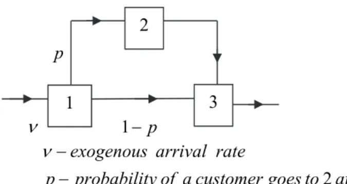
Using this method (Kiessler et al., 1988) achieved to show that, in a Jackson three node acyclic network, see Figure 1, the total sojourn time distribution function for a customer that follows

(6)

Aplimat – Journal of Applied Mathematics 222 volume 5 (2012), number 3 p  1 p 1 2 after to goes customer a of y probabilit p rate arrival exogenous   

Figure 1: Jackson Three Node Acyclic Network

the path integrated by the nodes 1, 2, and 3 is not the same obtained considering that , and the sojourn times at nodes 1, 2 and 3 respectively are independent although this one, designated by , is a “good” approximation of that one. They show that in some particular cases it was not true that

, 0 21

being and the minorant and the majorant, respectively, of that customer sojourn time distribution function, obtained through the described method.

This conclusion is important because, in spite of the dependence between and , see for instance (Ferreira, 2010), could be the distribution function. In fact, (Feller,

1966) presents an example of dependent random variables which sum has the same distribution as if the random variables were independent.

Finally note that the formula (12), apparently new, seems to be of great efficiency, although only allows to obtain moments minorants, because its field of application is a broad one.

References

ANDRADE, M.: A Note on Foundations of Probability. Journal of Mathematics and Technology, vol.. 1 (1), pp 96-98, 2010.

[2] ÇINLAR, E.: Introduction to Stochastic Processes. Prentice-Hall, Englewood Cliffs, New Jersey, 1975.

[3] DISNEY, R. L. and KÖNIG, D.: Queueing Networks: A Survey of their Radom Processes. SIAM Review, 3, pp. 335-403, 1985.

[4] FELLER, W.: An Introduction to Probability Theory and its Applications. Vol. II, John Wiley & Sons, New York, 1966.

[5] FERREIRA, M. A. M.: O Tempo de Permanência em Redes de Jackson. Revista de Estatística, 2 (2), pp. 25-44, 1997.

[6] FERREIRA, M. A. M.: Correlation Coefficient of the Sojourn Times in Nodes 1 and 3 of Three Node Acyclic Jackson Network. Proceedings of the Third South China International Business Symposium. Vol. 2. Macau, Hong-Kong, Jiangmen (China), pp. 875-881, 1998.

1

2

(7)

volume 5 (2012), number 3 223

[7] FERREIRA, M. A. M.: A note on Jackson Networks Sojourn Times. Journal of Mathematics and Technology, vol.. 1 (1), pp 91-95, 2010.

[8] FERREIRA, M. A. M. and ANDRADE, M.: Fundaments of Theory of Queues. International Journal of Academic Research, Vol. 3 (1, part II), pp. 427-429, 2011.

[9] FERREIRA, M. A. M. and ANDRADE, M.: Stochastic Processes in Networks of Queues

with Losses: A Review. International Journal of Academic Research, Vol. 3 (2, part IV), pp.

989-991, 2011.

[10] FERREIRA, M. A. M. and ANDRADE, M.: Grouping and Reordering in a Server Series. Journal of Mathematics and Technology, Vol 2 (2), pp. 4-8, 2011a.

[11] FERREIRA, M. A. M. and ANDRADE, M.: Non-Homogeneous Networks of Queues. Journal of Mathematics and Technology, Vol 2 (2), pp. 24-29, 2011b.

[12] FOLEY, R. D. and KIESSLER, P. C.: Positive Correlations in a Three-Node Jackson

Queueing Network. Advanced Applied Probability, 21, pp. 241-242, 1989.

[13] JACKSON, J. R.: Network of Waiting Lines. Operations Research, 5, pp. 518-521, 1957. [14] JACKSON, J. R.: Jobshop-like Queueing Systems. Management Science, 10, pp. 131-142, 1963.

[15] KELLY, F. P.: Reversibility and Stochastic Networks. John Willey & Sons, New York, 1979.

[16] KIESSLER, P. C., MELAMED, B., YADIN, M. and FOLLEY, R. D.: Analysis of a Three

Node Queueing Network. Queueing Systems, 3, pp. 53-72, 1988.

[17] LEMOINE, A. J.: On Sojourn Time in Jackson Networks of Queues. Journal of Applied Probability, 24, pp. 495-510, 1987.

[18] MELAMED, B. and YADIN, M.: Randomization Procedures in the Computation of

Cumulative-Time Distributions over Discrete State Markov Processes. Operations Research, 4 (32),

pp. 926-944, 1984.

[19] MELAMED, B. and YADIN, M.: Numerical Computation of Sojourn-Time Distributions in

Queueing Networks. Journal of the Association for Computing Machinery, 4 (31), pp. 839-854,

1984a.

Current address

Marina Andrade, Professor Auxiliar ISCTE – Lisbon University Institute UNIDE - IUL

Av. Das forças armadas 1649-026 Lisboa

Telefone: + 351 21 790 34 05 Fax: + 351 21 790 39 41

e-mail: marina.andrade@iscte.pt

Manuel Alberto M. Ferreira, Professor Catedrático ISCTE – Lisbon University Institute

UNIDE - IUL

Av. Das forças armadas 1649-026 Lisboa

TELEFONE: + 351 21 790 37 03 FAX: + 351 21 790 39 41

(8)