DOI: http://dx.doi.org/10.1590/2446-4740.01817 Volume 34, Number 1, p. 73-86, 2018
Introduction
ECG signals represent the heart electrical activity and they are obtained through electrodes placed in specific regions of the human body. There are five main waves characterizing ECG signals: P, Q, R, S, and T. Each wave or complex has an exclusive significance. The combination of Q, R and S waves forms which is known as QRS complex. The P wave and the QRS complex represent the atrial and ventricular depolarization, respectively. On the other hand, the T wave characterizes
the ventricular repolarization. The spectrum of the QRS complex is located in the ECG frequency bands whose typical frequency components range from 10 Hz to 25 Hz (Köhler et al., 2002) and its detection is still subject of many studies. Pan and Tompkins (1985) developed an objective QRS detection algorithm using a band-pass filter from 5 Hz to 12 Hz. Zidelmal et al. (2012) computed the power spectrum for four QRS types concluding that their energies are concentrated in the range from 5 Hz to 22 Hz. Such spectral information is used to QRS complexes detection in Challenge 2011 (Training Set A) database (Oliveira et al., 2015). In addition, it is important to remark that ECG signals are non-stationary, non-symmetric in relation to the x-axis and are originally impulsive signals (Łęski and Henzel, 2005).
The specific morphology of the ECG signals allows identifying various cardiac diseases. However, for an accurate analysis, signals should have high Signal-to-Noise Ratio (SNR) (Łęski and Henzel, 2005). Low SNR can difficult the analysis performed by experts or computational applications, since it changes the signal waveform. Typical noise present in ECG signals are due to power-line
A wavelet-based method for power-line interference removal in ECG signals
Bruno Rodrigues de Oliveira
1*, Marco Aparecido Queiroz Duarte
2, Caio Cesar Enside de Abreu
3,
Jozue Vieira Filho
41 Department of Electrical Engineering, São Paulo State University, Ilha Solteira, SP, Brazil. 2 Department of Mathematics, Mato Grosso do Sul State University, Cassilândia, MS, Brazil. 3 Department of Computing, Mato Grosso State University, Alto Araguaia, MT, Brazil. 4 São Paulo State University, São João da Boa Vista, SP, Brazil.
Abstract Introduction: The analysis of electrocardiogram (ECG) signals allows the experts to diagnosis several cardiac
disorders. However, the accuracy of such diagnostic depends on the signals quality. In this paper it is proposed a simple method for power-line interference (PLI) removal based on the wavelet decomposition, without the use
of thresholding techniques. Methods: This method consists in identifying the ECG and noise frequency range
for further zeroing wavelet detail coefficients in the subbands with no ECG coefficients in the frequency content. Afterward, the enhanced ECG signal is obtained by the inverse discrete wavelet transform (IDWT). In order to choose the wavelet function, several experiments were performed with synthetic signals with worse Signal-to-Noise
Ratio (SNR). Results: Considering the relative error metrics and runtime, the best wavelet function for denoising
was Symlet 8. Twenty synthetic ECG signals with different features and eight real ECG signals, obtained in the Physionet Challenge 2011, were used in the experiments. Results show the advantage of the proposed method against thresholding and notch filter techniques, considering classical metrics of assessment. The proposed method performed better for 75% of the synthetic signals and for 100% of the real signals considering most of the evaluation measures, when compared with a thresholding technique. In comparison with the notch filter, the
proposed method is better for all signals. Conclusion: The proposed method can be used for PLI removal in ECG
signals with superior performance than thresholding and notch filter techniques. Also, it can be applied for high frequencies denoising even without a priori frequencies knowledge.
Keywords Power-line interference, Denoising ECG signals, Wavelet decomposition.
This is an Open Access article distributed under the terms of the Creative Commons Attribution License, which permits unrestricted use, distribution, and reproduction in any medium, provided the original work is properly cited.
How to cite this article: Oliveira BR, Duarte MAQ, Abreu CCE,
Vieira Filho J. A wavelet-based method for power-line interference removal in ECG signals. Res Biomed Eng. 2018; 34(1):73-86. DOI: 10.1590/2446-4740.01817.
*Corresponding author: Department of Electrical Engineering, São
Paulo State University, Avenida 56, Centro, CEP 15385-000, Ilha Solteira, SP, Brazil. E-mail: [email protected]
interference in a frequency band varying from 50 Hz to 60 Hz (Łęski and Henzel, 2005; Patil and Chavan, 2012; Rahman et al., 2010) depending on the country. It occurs due to interferences of electrical equipment as X-ray, air conditioners, elevators (Patil and Chavan, 2012), and also due to the differences in electrode impedances
(Bahoura and Ezzaidi, 2010).
Several researchers have proposed denoising approaches to enhance ECG signals and preserve their original characteristics. Some noise reduction techniques are based on digital filters, wavelet transform and adaptive filtering (AlMahamdy and Riley, 2014); singular value decomposition (Bandarabadi and Karami-Mollaei, 2010); independent component analysis (Phegade and Mukherji, 2013) and S-transform (Das and Ari, 2013). Among the algorithms for PLI removal there are digital processing methods based on: fuzzy thresholding (Üstündağ et al., 2012); nonlinear filter bank (Łęski and Henzel, 2005); Fast Fourier Transform and adaptive nonlinear noise estimator (Shirbani and Setarehdan, 2013); Empirical Mode Decomposition (Agrawal and
Gupta, 2013); neural networks (Mateo et al., 2008)
and wavelet transform (Agrawal and Gupta, 2013; Garg et al., 2011; Poornachandra and Kumaravel, 2008; Rahman et al., 2010).
Wavelet analysis has been successfully used for ECG signal denoising because it deals well with non-stationary signals and also presents better resolution in time-frequency domain than Fourier analysis (Rahman et al., 2010). In the comparative study presented by AlMahamdy and Riley (2014), the wavelet transform produced better results in most of the experiments. Chouakri et al. (2006) compared the performance of Butterworth filters and the multilevel wavelet transform, concluding that improved results were achieved by the wavelet technique. Usually, wavelet-based methods for ECG denoising use thresholding techniques with some additional processing (Agante and Sa, 1999; AlMahamdy and Riley, 2014; Awal et al., 2014; Bahoura and Ezzaidi, 2010; Chouakri et al., 2006; Garg et al., 2011; Germán-Salló, 2010; Karthikeyan et al., 2012; Li et al., 2009; Patil and Chavan, 2012; Poornachandra and Kumaravel, 2008; Üstündağ et al., 2012). Patil and Chavan (2012) compared the PLI removal for different wavelet basis using hard and soft shrinkage functions. They conclude that hard thresholding achieves better SNR scores than soft thresholding, and the best wavelet basis depends on the analyzed signal.
Garg et al. (2011) worked on optimal wavelet-based algorithm for ECG denoising, analyzing SNR for several wavelet families, decomposition level and threshold selection method. In order to calculate the threshold, four rules were used: min-max, rigorous sure, universal and heuristic sure. The best configuration was achieved with the Symlet wavelet with ten vanishing moments
and five decomposition levels, hard shrinkage function and heuristic sure rule or rigorous sure thresholding.
Poornachandra and Kumaravel (2008) proposed to
use of hyper shrinkage function in the subbands that contained the PLI noise at some decomposition level. The obtained results were better when compared to those of the state-of-the-art algorithms.
In this paper, it is proposed to use discrete wavelet transform (DWT) to decompose an ECG signal degraded by high power-line interference. The goal is to have the ECG signal represented by the approximation coefficients and the noise by the detail coefficients. The basic idea is to inspect the ECG and noise frequency range in each subband of the wavelet filter bank. The wavelet scale whose frequency range exceeds the maximum frequency of the ECG signals is set to zero. Then, the IDWT is applied in order to obtain a better quality signal without the use of thresholding techniques. It is common that such techniques do not completely eliminate noise, generating residual noise that can still distorts the QRS waveform. Therefore, this original ECG analysis methodology eliminates the need of thresholding function and is based solely on wavelet filter bank and the characteristics of PLI. Comparisons with a thresholding technique and a classical digital filter were carried out to demonstrate the effectiveness of the proposed method. Furthermore, the proposed method presents low computational load, reduces the residual noise and can be easily implemented.
Methods
A noisy ECG, s t( ), contaminated by PLI can be represented as follows:
( ) ( ) cos 2( r )
s t =x t + α π + ϕf t , (1)
where t is time and fr=50 Hz or fr= 60 Hz is the PLI frequency. The unknown parameters are ϕ∈ 0, 2
[
π]
, PLI signal phase and α > 0, the amplitude. The clean ECG is represented by x t( ).Dynamical model for generating synthetic ECG signals
around the “attracting limit cycle of unit radius” describes the ECG signal for each RR-interval (McSharry et al., 2003). ECG characteristic waves are events with fixed angles in relation to the unit circle, given by θi, for
{ , , , , }
i∈ P Q R S T . The ODE model (McSharry et al., 2003) is given by y= −
(
1 x2+y2)
y+ ρx, x= −(
1 x2+y2)
x− ρxand ( )
2
2 2
exp 0.15sin 2
2 i i i
i i
z a z f
b ∆θ
= −∑ ∆θ − − − π
, where
( ) 2 ,
atan x y
θ = and atan2( )x y, is the element-by-element arctangent between x and y arrays, ∆θ = θ − θi ( i), ρ is the angular trajectory velocity and f2 is the respiratory frequency for modeling the baseline wander. z is the generated ECG itself.
This dynamical model yields realistic signals when compared to real ECG signals (McSharry et al., 2003). By setting parameters a bi, , iθi and f2, different morphologies can be generated for ECG characteristic waves. Note that z is a superposition of sinusoidal and Gaussian functions. Therefore, parameters ai and bi affect the amplitude and
the width of the simulated ECG waves, respectively. Some specific features of the heart rate can also be set, such as mean and standard deviation, besides spectral properties. Generated waveforms are similar
to the 12-lead ECG lead I. Although it is possible to produce multi-lead signals (McSharry et al., 2003), in this work they were not considered.
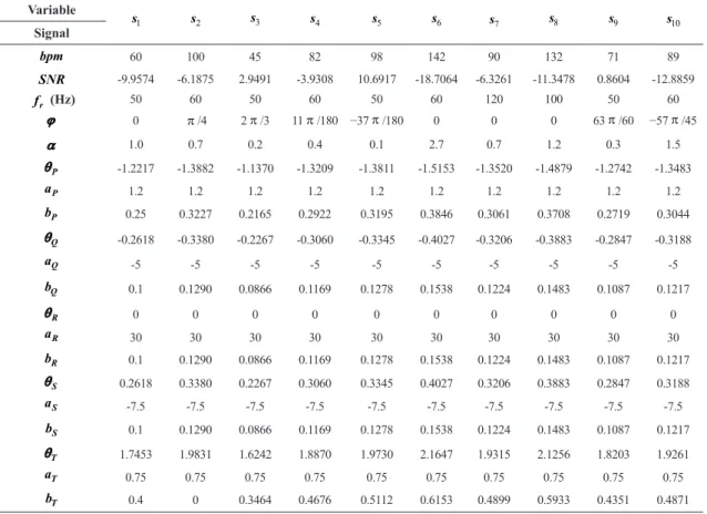
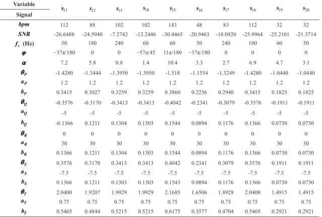
In order to set parameters of the proposed method and perform experiments for validation, twenty synthetic signals were generated using the described model. Model parameters and features of the generated ECG signals are summarized in Table 1 and Table 2. All signals were sampled at fs 500= Hz, in an interval of 60 seconds (30001 samples). Parameters were set for the dynamical model in order to obtain ECG signals with different heart rate, SNR and PLI values. By using different settings, it was possible to obtain ECG waveforms with different lengths, amplitudes and fiducial points. Noise was added to each synthetic signal according to equation (1), considering the parameters described in Table 1 and Table 2. Such parameters simulate different PLI noises which can be found in a real ambulatory (Huhta and Webster, 1973), unlike the most state-of-the-art methods which focus on pure sinusoidal noise. So, in addition to the fundamental frequency, harmonics interferences were also considered (Costa and Tavares, 2009).
Table 1. ECG synthetic signals configuration using the model described in this section. Parameters: r
f is PLI frequency; ϕ and α are noise phase
and noise amplitude, respectively; other parameters refer to the dynamical model.
Variable
1
s s2 s3 s4 s5 s6 s7 s8 s9 s10
Signal
bpm 60 100 45 82 98 142 90 132 71 89
SNR -9.9574 -6.1875 2.9491 -3.9308 10.6917 -18.7064 -6.3261 -11.3478 0.8604 -12.8859
r
f (Hz) 50 60 50 60 50 60 120 100 50 60
ϕ 0 π/4 2π/3 11π/180 −37π/180 0 0 0 63π/60 −57π/45
α 1.0 0.7 0.2 0.4 0.1 2.7 0.7 1.2 0.3 1.5
P
θ -1.2217 -1.3882 -1.1370 -1.3209 -1.3811 -1.5153 -1.3520 -1.4879 -1.2742 -1.3483
P
a 1.2 1.2 1.2 1.2 1.2 1.2 1.2 1.2 1.2 1.2
P
b 0.25 0.3227 0.2165 0.2922 0.3195 0.3846 0.3061 0.3708 0.2719 0.3044
Q
θ -0.2618 -0.3380 -0.2267 -0.3060 -0.3345 -0.4027 -0.3206 -0.3883 -0.2847 -0.3188
Q
a -5 -5 -5 -5 -5 -5 -5 -5 -5 -5
Q
b 0.1 0.1290 0.0866 0.1169 0.1278 0.1538 0.1224 0.1483 0.1087 0.1217
R
θ 0 0 0 0 0 0 0 0 0 0
R
a 30 30 30 30 30 30 30 30 30 30
R
b 0.1 0.1290 0.0866 0.1169 0.1278 0.1538 0.1224 0.1483 0.1087 0.1217
S
θ 0.2618 0.3380 0.2267 0.3060 0.3345 0.4027 0.3206 0.3883 0.2847 0.3188
S
a -7.5 -7.5 -7.5 -7.5 -7.5 -7.5 -7.5 -7.5 -7.5 -7.5
S
b 0.1 0.1290 0.0866 0.1169 0.1278 0.1538 0.1224 0.1483 0.1087 0.1217
T
θ 1.7453 1.9831 1.6242 1.8870 1.9730 2.1647 1.9315 2.1256 1.8203 1.9261
T
a 0.75 0.75 0.75 0.75 0.75 0.75 0.75 0.75 0.75 0.75
T
Table 2. ECG synthetic signals configuration using the model described in this section. Parameters: fr is PLI frequency; ϕ and α are noise phase
and noise amplitude, respectively; other parameters refer to the dynamical model.
Variable
11
s s12 s13 s14 s15 s16 s17 s18 s19 s20
Signal
bpm 112 88 102 102 143 48 83 112 32 32
SNR -26.6488 -24.5940 -7.2742 -12.2446 -30.4465 -20.9463 -18.0920 -25.9964 -25.2101 -21.3714
r
f (Hz) 50 180 240 60 60 50 240 100 60 50
ϕ −37π/180 0 0 −57π/45 11π/180 −37π/180 0 0 0 0
α 7.2 5.8 0.8 1.4 10.4 3.3 2.7 6.9 4.7 3.1
P
θ -1.4280 -1.3444 -1.3950 -1.3950 -1.518 -1.1554 -1.3249 -1.4280 -1.0440 -1.0440
P
a 1.2 1.2 1.2 1.2 1.2 1.2 1.2 1.2 1.2 1.2
P
b 0.3415 0.3027 0.3259 0.3259 0.3860 0.2236 0.2940 0.3415 0.1825 0.1825
Q
θ -0.3576 -0.3170 -0.3413 -0.3413 -0.4042 -0.2341 -0.3079 -0.3576 -0.1911 -0.1911
Q
a -5 -5 -5 -5 -5 -5 -5 -5 -5 -5
Q
b -0.1366 0.1211 0.1304 0.1303 0.1544 0.0894 0.1176 0.1366 0.0730 0.0730
R
θ 0 0 0 0 0 0 0 0 0 0
R
a 30 30 30 30 30 30 30 30 30 30
R
b 0.1366 0.1211 0.1304 0.1303 0.1544 0.0894 0.1176 0.1366 0.0730 0.0730
S
θ 0.3576 0.3170 0.3413 0.3413 0.4042 0.2341 0.3079 0.3576 0.1911 0.1911
S
a -7.5 -7.5 -7.5 -7.5 -7.5 -7.5 -7.5 -7.5 -7.5 -7.5
S
b 0.1366 0.1211 0.1303 0.1303 0.1543 0.0894 0.1176 0.1366 0.0730 0.0730
T
θ 2.0400 1.9207 1.9929 1.9929 2.1685 1.6506 1.8928 2.0400 1.4915 1.4915
T
a 0.75 0.75 0.75 0.75 0.75 0.75 0.75 0.75 0.75 0.75
T
b 0.5465 0.4844 0.5215 0.5215 0.6175 0.3577 0.4704 0.5465 0.2921 0.2921
Real ECG signals
In order to validate the proposed method using real ECG signals that have been originally corrupted by PLI, the Challenge 2011 (Training Set A) database from Physionet was chosen (Goldberger et al., 2000). Their records were sampled at 500 Hz with 16-bit resolution, during 10 seconds, for standard 12-lead (leads I, II, III, aVR, aVL, aVF, V1, V2, V3, V4, V5, V6) and their parameters are summarized in Table 3. Note from Table 3 that Power Spectral Density (PSD) column is the sum of the power spectrum density only for frequencies
over 25 Hz, and it is expressed as 4
10
PSD× decibels (dB).
Discrete wavelet transform
The wavelet analysis has been applied to various problems in biomedical engineering including noise removal in ECG signals (Agante and Sa, 1999; AlMahamdy and Riley, 2014; Awal et al., 2014; Bahoura and Ezzaidi, 2010; Chouakri et al., 2006; Garg et al., 2011; Germán-Salló, 2010; Karthikeyan et al., 2012; Li et al., 2009; Patil and Chavan, 2012; Poornachandra and Kumaravel, 2008; Üstündağ et al., 2012). Due to its better time-frequency resolution, it overcomes other classical methods, such as short time Fourier Transform, for instance (Üstündağ et al., 2012). One of the advantages when using wavelets is
the computational efficiency of Mallat’s pyramidal algorithm (Mallat, 1989). This algorithm is indeed a two-channel filter bank that splits the input signal in low and high frequencies by using quadrature mirror filters. The filters can be described through the wavelet ψ( )t and the scaling φ( )t basis functions (Mallat, 1989):
( ) / 2 ,
2 2
2 j j
j n j
t n
t − −
ψ = ψ
, (2)
( ) / 2 ,
2 2
2 j j
j n j
t n
t − −
φ = φ
, (3)
1/ 2
[ ] 2 ( / 2), ( )
h n = − φt φt−n , (4)
[ ]
21/ 2 ( / 2 ,) ( )g n = − ψ t φ t−n , (5)
where
[ ]
( )1[
]
1 n 1
g n = − − h −n, j=1, 2,…,J and n integer. Such basis functions satisfy the conditions ( )2
1 t dt
∫ φ =
(Mallat, 2009) and ∫ ψ( )t dt=0 (Daubechies, 1992). For a discrete analysis, wavelets are constructed by discretizing a “mother” function, and scaling it by 2j (Mallat, 2009), according to Equations (2) and (3). In this way, a signal
( )
[ ]
( ), , ( )j j n
d n = x t ψ t (6)
and
[ ]
( ), , ( )j j n
a n = x t φ t , (7)
where a nj
[ ]
and dj[ ]
n are, respectively, the j-thapproximation and detail coefficients at scale 2j, and j is the decomposition level. In a general way, given two sequences f n1
[ ]
and f2[ ]
n, their inner product is defined as f1,f2 = ∫f t f1( ) ( )2 t dt, where f2( )t is the complex conjugate of f2( )t . These coefficients can be computed in a fast way by a cascade algorithm, using discrete convolutions and subsamplings, by means of[ ]
[ ]
1 * 2
j j
a+ p =a h p and dj+1
[ ]
p =a nj[ ] [ ]
*g 2p (Mallat,2009), where x n
[ ] [ ]
= −x n, p is an integer and * is the convolution operation. This operation means coefficients filtering in a lower resolution, i.e., j. In this way, h[ ]
2p filters the higher frequencies and g[ ]
2p lets them pass. Therefore, an orthogonal representation for a signal( )
x t is composed by the largest scale approximation
coefficients plus detail coefficients at the scales j (Mallat, 2009), as follows:
( ) J
[ ]
J n, ( ) j[ ]
j n, ( )n j J n
x t a n t d n t
≤
=∑ φ +∑ ∑ ψ . (8)
Therefore, the wavelet decomposition output is a smooth signal representing the original one in a coarse way. In addition, the details are obtained when moving from a lower to a higher scale. Note that the smooth signal and details represent the similarity between the scaling and wavelet functions, according to Equations (7) and (6), respectively. For an ECG signal, the approximation coefficients represent its smoothed version. On the other hand, detail coefficients capture abrupt changes, such as high-frequency noises. In order to reconstruct the signal
( )
x t the following equation is required (Mallat, 2009):
[ ]
1*[ ]
1*[ ]
j j j
a p =a+ h p +d+ g p, where y n[ ]=0 if n=2p+1 or y n[ ] [ ]=y p if n=2p.
In the analysis step, the output wavelet filter bank frequency spectrum is divided into two octave bands. In each new decomposition level, the low-frequency spectrum is again divided into two new octave bands, at the ideal cut-off frequencies, and so on, resulting in a logarithmical set of bandwidth (Germán-Salló, 2010). Therefore, if fs is the sampling frequency, the frequency
contents for approximation and detail coefficients, in the j-th decomposition level, are in the interval 0, / 2j 1
s
f +
and 1
/ 2j , / 2j
s s
f + f
, respectively. In practice, the ideal
cut-off frequencies are not realizable (Peng et al., 2009). Therefore, the intervals are not exactly those mentioned before. Abrupt changes in the frequency intervals do not occur, but the filters frequency responses magnitude decreases gradually, tending to a constant value. Thus, leakage energy affects the frequency content for each DWT decomposition subband. Approximation
coefficients are scattered higher than 1
/ 2j
s
f + frequencies.
On the other hand, detail coefficients are lower than 1
/ 2j
s
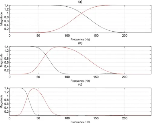
f + frequencies and higher than fs/ 2j. Hence, there is a band overlap. Therefore, DWT frequency behavior impacts the decomposition level and the wavelet function choices. As an example, Figure 1 shows the frequency content for the quadrature mirror analysis filters given by Equations (2) and (3) for a 500 Hz sampling rate.
Thresholding techniques
Classical methods for ECG denoising based on thresholding techniques present good performances
(AlMahamdy and Riley, 2014; Garg et al., 2011; Patil
and Chavan, 2012; Poornachandra and Kumaravel, 2008). Basically, in such methods, the goal is to estimate the signal x t( ) from a contaminated signal s t( ) ( ) ( ) =x t +r t , where r t( ) is the additive noise (Donoho and Johnstone, 1994). For this purpose, the DWT is applied to s t( ) and then dj
[ ]
n = s t( ),ψj n, ( )t in the wavelet domain is obtained. For hard shrinkage function, the absolute value of dj[ ]
n is compared to a threshold λ. If dj[ ]
n ≤λ, thecorresponding value associated to the index n is set to 0. Otherwise, it is preserved.
In order to implement the wavelet shrinkage method, it has considered the Symlet 8 wavelet with three DWT decomposition levels and universal threshold (given by
( )
2 log N
λ = , where N is the signal length), combined
with hard thresholding function. It is noteworthy that this is the best configuration for this method (Garg et al., 2011; Patil and Chavan, 2012). The choice of the wavelet function order and the number of decomposition levels are justified since they are the same used by the proposed method.
Notch filter
McManus et al. (1993) present four categories of digital filters for PLI removal: low-pass, notch-rejection, adaptive and global. For the implementation of the Table 3. Parameters of the real ECG signals.
Record (Lead) eSQI stdSQI PSD (dB)
1007823 (II) 0.6460 0.2051 -1.5345
1034914 (III) 0.3982 0.1875 -1.2290
1086219 (III) 0.3969 0.2147 -1.3232
1098605 (V1) 0.4421 0.2969 -1.3742
1105115 (V2) 0.4136 0.1507 30.7853
1124627 (aVL) 0.5272 0.1676 -1.0693
2209843 (I) 0.5557 0.2565 -1.5421
1138505 (I) 0.4139 0.3344 -1.2085
narrow-band-rejection filter (notch) it is considered a recursive filtering that includes a two-pole and two-zero filter. The filter output is given by
( ) ( )
1(
1)
2(
2)
3(
1)
4(
2)
y k =x k +a x k− +a x k− +a y k− +a y k−
wherex k( ) is the input ECG signal and the
coefficients are a1= −2 1( − πBC/fs) ( )cosθ, ( )
2
2 1 / s ,
a = − πBC f
( ) ( )
3 2 1 / s cos
a = − πB f θ and a4= − − π(1 B/ fs)2, in which
2 fnom/ fs
θ = π , and B C f, , nom, fs are -3 dB response bandwidth (in Hz), center-frequency response, PLI frequency and sampling rate, respectively (McManus et al., 1993, apud Lynn, 1971).
In order to compare the proposed method with a classical approach, the recursive notch filter was selected. Lynn (1971) apud McManus et al., (1993), set
10
B≈ Hz, C≈0.01 and fs=1 kHz. Such parameters do not assure the best results for the signals tested in this work. Therefore, they were empirically set as B=5 Hz,
0.005
C= and fs=500 Hz, assuring best results. Considering that the objective of this work is to introduce a new method that overcomes the thresholding techniques, the results were compared to the ones obtained by a classical approach.
Evaluation metrics
In the literature, many objective measures are proposed to assess denoising techniques. One of them is the SNR,
given by
(
2 2)
10 10 log x/ y
SNR= σ σ dB where 2
x
σ and 2
y
σ are,
respectively, signal and noise variances. For a signal ( )
x t, the SNR improvement is defined by Awal et al.
(2014) as SNRimp=10log10∑s t( ) ( )−x t 2/∑x tˆ( ) ( )−x t 2 dB, where x tˆ( ), s t( ) and x t( ) represents the denoised signal, noisy signal and original ECG signal, respectively. Another measure, associated with mean square error is the root mean square error (RMSE) expressed by
( ) ( ) 2 ˆ
1 /
RMSE= N∑x t −x t, where N is the signal length. The relative error in the signal estimation can be written as ε =1 /N∑x tˆ( ) ( )−x t . A statistical measure that allows the linear association between the predicted signal and the original one is the correlation coefficient (Üstündağ et al.,
2012): ( ) ( ) ˆ ( ) ( ) ˆ
2 2
ˆ / ˆ
x x x x
r= ∑x t − µ x t − µ ∑x t − µ ∑x t − µ,
where µx and µxˆ are the expected values for x t( ) and ( )
ˆ
x t, respectively. This measure varies from −1 to 1 and the zero means no linear relationship.
The measures presented before are appropriate for synthetic ECG signals, but not for real signals, since, in that case, there is no prior access to noiseless ECG signals samples. In this way, two metrics, proposed by Li et al. (2014), are used: the relative QRS complexes energy, given by eSQI= ∑Er Eai/ , and the relative standard deviation, given by stdSQI= ∑ σ( ri) / 2M aσ i, where Ea is the energy of the whole signal, Er is the i
energy in each QRS complex, M is the total number of Figure 1. Frequency response for the quadrature mirror analysis filters in Equations (2) (black line) and (3) (red line) for Symlet 8-tap wavelet in
QRS complexes, σri is the standard deviation of each
QRS complex and σai is the standard deviation around the i-th QRS complex (from: R− 0.2s to R 0.2s+ ; where R is the location of each R peak).
Statistical analysis
In order to evaluate whether the differences among the means in the experimental results are merely due to some random samples in the population, it is used the Kruskal-Wallis test. In this statistical test, ranks are used instead of the original observations. Firstly, all observations are ranked together and then the sum of the ranks is computed for each sample by means of the
equation: ( ) 2 ( )
1 12 3 1 1 N i i i
i i i
R
H n
n n = n
= ∑ − ∑ +
∑ ∑ + , where N is the
number of samples, ni is the number of the observations
and Ri is the sum of ranks in the i-th sample (Kruskal
and Wallis, 1952). H corresponds to some value in the 2
χ distribution. Thus, the probability to get a highest
or equal value than H is given by 2
1
PrχN− ≥H, that is
named p-value, with N−1 degrees of freedom. When H is large and -valuep ≤ α, then the null hypothesis is rejected (Kruskal and Wallis, 1952). In our case, the null hypothesis is that there is no significant difference among the tested methods. In this work α =0.05.
Proposed method
According to equation (1), the ECG signal represented by s t( ) is added to another signal which represents the PLI. Thus, an estimated ECG signal x tˆ( ) can be obtained as follow:
( ) ( ) cos( )
ˆ 2 r
x t =s t − α π + ϕf t . (9)
In the wavelet domain, the signal s t( ) is represented by the approximation coefficients and PLI is contained in detail coefficients for a specific subband. Consequently, a simple approach to enhance the ECG signal in the wavelet domain is to reconstruct the signal x tˆ( ) discarding detail coefficients. Based on the wavelet representation, Equation (8), the signal x tˆ( ) can be written as a product comprising scaling functions and low-pass filter outputs added to the sum of the product of wavelet functions and high-pass filter outputs. In the j-th level, low-frequency components are limited in the interval 0, /2j 1
s
f +
while the high-frequency components are in interval 1
/2j , /2j
s s
f + f
. Note that the precise frequency spectrum
partition is impractical, since the filters frequency responses should be ideal (Peng et al., 2009). It results in a band
overlap with frequency content close to 1
/2j
s
f +. In the
overlap band interval the energy leakage occurs when the wavelet decomposition is used (Peng et al., 2009), i.e., besides the expected frequency components, other frequencies also appear in the decomposed signal.
Peng et al. (2009) solved this problem by resampling the signal when the frequency content of interest is in
the neighborhood of 2
2 fs
− .
Choosing fs in a such a way that the approximation
coefficients spectrum is limited in the range
[
0, 25.0]
Hz and for detail coefficients spectrum is limited in the range[ ]
a b, , where a 25≥ Hz and b 60≥ Hz, for some decomposition level j, and 22fs 25− > Hz, it is possible to separate, in
the wavelet domain, the PLI noise from the corrupted ECG signal. Obviously, the choice of j depends on the ECG signal sampling rate fs. According to Nyquist’s
Theorem, fs should satisfy the following inequality:
2
s N
f ≥ f , where fN is the maximum frequency of the
signal. For instance, if fs=125 Hz then fN=62.5 Hz, and therefore if j=1, approximation coefficients are in the range
[
0, 31.25]
Hz, which comprises the frequency range content in an ECG signal. Detail coefficients are in the range[
31.25, 62.5]
Hz, containing PLI noise and other high-frequency noises.As suggested by Peng et al. (2009), the upper limit for the approximation coefficients is higher than 25 Hz, which is the frequency of interest. Therefore, setting the sampling rate at 125 Hz is suitable. Obviously, for other sampling rates that are integer multiple of 125 Hz, the ECG signal and PLI noise can also be separated, but for higher decomposition levels. Nevertheless, for the experiments performed in this work the best results were obtained at a sampling frequency of 500 Hz. In Table 4 it is shown the frequency distribution in each decomposition level for such sampling rate. Columns two and three show the frequency range for ideal cut-off frequencies according to the range shown in the Figure 1. Columns four and five show the real ranges, which are approximated values, obtained by analyzing the frequency response with the Symlet 8-tap. In the column six are presented the approximate band overlap ranges, considering the quadrature mirror analysis filters from Equations (4) and (5).
In a noise-free ECG signal reconstruction, detail coefficients are not so important, since they do not have relevant information about the ECG signal waveform, as shown in Table 4. Therefore, in order to obtain the signal x tˆ( ), given the sampling rate fs, a decomposition level L≤J must be chosen, where J is the maximum level. Afterward, it is assumed dj
[ ]
n =0, for all n and1 , 2, ,
j= L in Equation (8). In this way, it follows from equation (8) that
( )
[ ]
, ( )ˆ L L n
n
x t =∑a nφ t . (10)
run; 4.1) DWT is applied to the splited signal, up to the level L; 4.2) set dj
[ ]
n =0 for all n and j=1, 2, , L; 4.3) The estimated ECG signal is reconstructed according to equation (10).The choice of the parameter L is the key to isolate the noise in a wavelet decomposition subband and that is why the sampling rate was defined as multiple of 125 Hz. If such sampling rate is not possible, there is no guarantee that the PLI will appear in the detail coefficients. In this way, resampling of the ECG signal should be considered. The null samples are added to avoid abrupt changes in the signal ends and W/ 2 samples are necessary due to the window overlap, which is an important procedure in signal processing. Generally, the window overlap vary from 50% to 75% (Prabhu, 2014), but for the proposed method better results were achieved with 50% overlapping.
Results
The wavelet function choice
When applying the wavelet transform, besides the decomposition level choice discussed in the last section, it is also important to choose the wavelet function that best fits the signal. When ECG is the subject and threshold based methods are used, some researchers prefer Symlet wavelets because their scaling function resembles more its waveform (Awal et al., 2014; Chouakri et al., 2006; Karthikeyan et al., 2012; Li et al., 2009). Good results are also found using Daubechies wavelets (Karthikeyan et al., 2012; Patil and Chavan, 2012; Üstündağ et al., 2012) and Coiflet (Agante and Sa, 1999; Karthikeyan et al., 2012). On the other hand, Poornachandra and Kumaravel (2008) compared some wavelet families with Mayer’s wavelet and conclude that the last one is better. Commonly, each method uses different thresholding techniques and they have influence on the wavelet function choice. However, there is some agreement about the use of Daubechies and Symlet wavelets. As the proposed method does not use thresholding techniques, the choice of wavelet function can be made by analyzing the results of experiments using the synthetic signals from Table 1 and Table 2. Preliminary experiments with the proposed method showed that the relative error obtained when using Symlets is smaller than the one using Daubechies wavelet functions. Furthermore, it was noted that higher
wavelet order leads to better result. However, runtime increases substantially.
For instance, the difference between the relative errors metrics, for the synthetic signal s1, using sym10 (Symlet wavelet function of order 10) and sym20 is
4
5.14 1× 0− and the absolute difference between runtimes
is around 2
2.17 1× 0− seconds. When s15 is considered, which is the one with worse SNR, runtime increases by about 10−3 seconds, from sym2 to sym8. From sym8
on, this metric increases by an amount of 1
10− seconds when the number of the wavelet vanishing moments increases. On the other hand, the relative error metric decreases in average 2 1×0−4 for each new Symlet wavelet function order, from sym4 on. Longer runtime is due to higher amount of the filters coefficients for wavelets of higher order.
Figure 2 shows the boxplots of the experiments for denoising synthetic signals with worse SNR:
6, , , , , , , 8 11 12 13 15 16 17
s s s s s s s s and s20. Each box displays the relative error and runtime for different Symlet wavelet orders. The higher the order of the wavelet, the larger the filter length and number of the vanishing moments. This implies on softer functions and higher runtime. In general, the relative error remains almost constant from sym8 on, according to the results presented. Conversely, runtime is almost constant for wavelet functions with order lower than 8, increasing significantly after sym8. Therefore, considering balance between the relative error and the runtime, the authors believe that the best results could be achieved using sym8.
Experiments
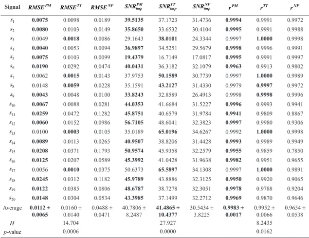
In order to validate the proposed method, evaluation measures were computed for each synthetic signal. According to the analysis in last section, Symlet 8 was used for simulations. Superscripts PM, TT and NF refer to proposed method, thresholding technique and notch filter, respectively.
Analyzing column eight in Table 5, it can be seen a significant SNR improvement (SNRimp) when compared to
the values from row two in Table 1 and Table 2. For s15 signal, with input SNR around −30 dB, the improvement was 50.9574 dB. s11, with input SNR around −26 dB, the
second worse, has an improvement of 45.8751dB. In a
general view, the SNRimpmetric has an average close to
40.7806 dB. The correlation coefficient r (eleventh Table 4. Frequency distribution for the wavelet decomposition of a signal sampled at 500 Hz considering a 3 dB cut-off frequency, according to Figure 1.
Level Ideal frequency range (Hz) Real frequency range (Hz) Band overlap range (Hz) Approximation Detail Approximation Detail
1 0-125 125-250 0-138.6 111.4-250 111.4-138.6
2 0-62.5 62.5-125 0-69.30 55.72-138.58 55.72-69.30
Figure 2. Boxplot for several Symlet wavelet orders: (a) relative error metrics boxplot, (b) runtime.
Table 5. Results for the proposed method (PM), thresholding technique (TT) and notch filter (NF) applied to synthetic ECG signal.
Signal PM
RMSE RMSETT RMSENF SNRimpPM
TT imp
SNR SNRimpNF rPM rTT rNF
1
s 0.0075 0.0098 0.0189 39.5135 37.1723 31.4736 0.9994 0.9991 0.9972
2
s 0.0080 0.0103 0.0149 35.8650 33.6532 30.4104 0.9995 0.9991 0.9988
3
s 0.0049 0.0018 0.0086 29.1643 38.0101 24.3344 0.9997 1.0000 0.9998
4
s 0.0040 0.0053 0.0094 36.9897 34.5251 29.5679 0.9998 0.9996 0.9991
5
s 0.0075 0.0103 0.0099 19.4379 16.7149 17.0817 0.9995 0.9991 0.9997
6
s 0.0190 0.0292 0.0474 40.0431 36.3182 32.1079 0.9963 0.9913 0.9802
7
s 0.0062 0.0015 0.0143 37.9753 50.1589 30.7739 0.9997 1.0000 0.9989
8
s 0.0148 0.0059 0.0228 35.1591 43.2127 31.4330 0.9979 0.9997 0.9972
9
s 0.0043 0.0048 0.0100 33.8243 32.8589 26.4913 0.9998 0.9998 0.9996
10
s 0.0067 0.0088 0.0281 44.0353 41.6684 31.5227 0.9996 0.9993 0.9941
11
s 0.0259 0.0472 0.1282 45.8751 40.6579 31.9784 0.9941 0.9809 0.8867
12
s 0.0060 0.0152 0.0986 56.7105 48.6041 32.3823 0.9997 0.9980 0.9306
13
s 0.0100 0.0003 0.0105 35.0189 65.0196 34.6267 0.9992 1.0000 0.9998
14
s 0.0089 0.0113 0.0265 40.9507 38.8206 31.4428 0.9993 0.9989 0.9949
15
s 0.0208 0.0371 0.1793 50.9574 45.9358 32.2579 0.9955 0.9859 0.7850
16
s 0.0125 0.0207 0.0589 45.3992 41.0428 31.9638 0.9982 0.9951 0.9655
17
s 0.0056 0.0010 0.0375 50.6373 65.5897 34.1308 0.9997 1.0000 0.9891
18
s 0.0245 0.0312 0.1182 45.9789 43.8886 32.3125 0.9950 0.9920 0.9065
19
s 0.0122 0.0385 0.0806 48.6787 38.7278 32.3051 0.9978 0.9788 0.9204
20
s 0.0148 0.0304 0.0534 43.3985 37.1499 32.2712 0.9969 0.9870 0.9646
Average 0.0112 ±
0.0065
0.0160 ±
0.0140 0.0488 ± 0.0471 40.7806 ± 8.2487 41.4865 ± 10.4377
30.5434 ±
3.8225 0.9983 ± 0.0017
0.9952 ±
0.0066 0.9654 ± 0.0538
H 14.704 27.927 8.2435
-value
p 0.0006 0.0000 0.0162
column) is close to one for all signals, meaning that the estimated signal waveform matches with the original ECG signal. Relative error ε and RMSE metrics indicate an accuracy of at least 2
10− for almost all experiments. In Figure 3, one can see the results in time and frequency domain, when applying the denoising methods for signal s15.
Figure 3. Analysis display for signal s15. (a) Synthetic ECG signal and (b) its spectrogram. (c) Noisy ECG signal and (d) its spectrogram. Denoised
ECG signals obtained by (e) proposed method, (g) thresholding technique and (i) notch filter, and their spectrograms (f), (h) and (j), respectively. The red rectangle highlights a distortion inserted by the thresholding technique.
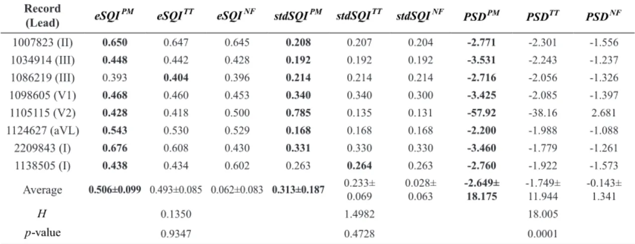
Table 6. Results for the proposed method, thresholding technique and notch filter applied to real ECG signals. PSD column is the sum of the power
spectrum density for frequencies over 25 Hz.
Record (Lead)
PM
eSQI eSQITT eSQINF stdSQIPM TT
stdSQI stdSQINF PM
PSD PSDTT PSDNF
1007823 (II) 0.650 0.647 0.645 0.208 0.207 0.204 -2.771 -2.301 -1.556
1034914 (III) 0.448 0.442 0.428 0.192 0.192 0.192 -3.531 -2.243 -1.237
1086219 (III) 0.393 0.404 0.396 0.214 0.214 0.214 -2.716 -2.056 -1.326
1098605 (V1) 0.468 0.460 0.453 0.340 0.340 0.300 -3.425 -2.085 -1.397
1105115 (V2) 0.428 0.418 0.500 0.785 0.135 0.131 -57.92 -38.16 2.681
1124627 (aVL) 0.543 0.530 0.529 0.168 0.168 0.168 -2.200 -1.988 -1.088
2209843 (I) 0.676 0.608 0.430 0.331 0.330 0.330 -3.460 -1.779 -1.261
1138505 (I) 0.438 0.434 0.602 0.263 0.264 0.263 -2.760 -1.922 -1.573
Average 0.506±0.099 0.493±0.085 0.062±0.083 0.313±0.187 0.233± 0.069 0.028± 0.063 -2.649±
18.175
-1.749±
11.944 -0.143± 1.341
H 0.1350 1.4982 18.005
-value
Discussion
Comparing the proposed method results to the ones obtained with hard thresholding method, it can be seen that the proposed method was worse than hard thresholding only for s3, s7,s8, s13 and s17 signals. In fact, the proposed method performed better in all requirements for all other signals. Average values reaffirm that the proposed method was better for the most of the evaluation measurements, except in terms of SNRimp. However, the
differences on SNRimp values were not significant. For this
metric, the proposed method was better than thresholding technique for 75% of the synthetic signals. In addition, it got higher results for signals s11 and s15, the ones with the worst SNR values.
By means of the Kruskal-Wallis test, we conclude that there exists significantly statistical difference for at least two methods. In comparison to notch filter, the proposed method was better for all measures. However, the proposed method and the thresholding technique have a similar performance in statistical terms.
Note, from Figure 3 (f), that the energy of the QRS complexes remains practically unchanged when compared to the original. The original signal energy is close to
3
3.2015 10× , whereas the energy of the denoised ECG signals obtained by the proposed method, thresholding technique and notch filter, are close to 3.2188 1× 03, 3.3894 1× 03
and 3
12.6194 1× 0, respectively. In addition, note from Figure 3 (g), that the thresholding technique inserted a distortion in the initial samples of the ECG signal whereas the proposed method did not change its waveform. Moreover, it can be seen from Figure 3, (i) and (j), that notch filter achieved poor performance, since PLI was only attenuated. In the signal first samples it cleared the PLI with biggest gain. This outcome is common for notch filter (Nauman et al., 2013). Due to the fact that some ECG analysis is performed by humans, a good visual quality is essential for an accurate diagnosis. Thus, one can conclude that the proposed method performed the best in terms of noise attenuation and distortion insertion.
For real ECG signals, from Table 6, it is notorious that the proposed method reached better results for all signals, except for record 1086219 with respect to eSQI and record 1138505 for stdSQI. It is still noticeable that eSQI measure values are greater for signals obtained by the proposed method than the ones for the original signals. Since this measure is directly proportional to the QRS complex energy, these results mean that the high frequency noises (60 Hz or 50 Hz) have their gain attenuated. Furthermore, the proposed method performed the best for most of ECG signals, and it is important to highlight that its computational complexity is lower, since the additional thresholding technique complexity due to threshold computation is O N( ) (Lang et al., 1996).
In comparison to notch filter, the proposed method obtained better results for all signals. It is noteworthy that notch filter performed the worst for all quality assessment tests.
From Kruskal-Wallis test results, it is noted that only for the PSD measure there are significantly statistical difference among the three methods, considering a level of significance of α =5%. This is because the other measures not consider the PLI noise.
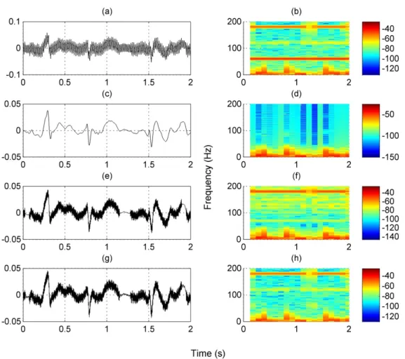
From Figure 4, one can observe that thresholding technique and notch filter removed the PLI only for some segments in the observed ECG signal, leaving the others attenuated. Hereby, the result for record 1105115 obtained by the proposed method is much better (Table 6, fifth row) than the other methods, since the high frequency noise (180 Hz, see spectrogram in Figure 4) was not removed by the thresholding technique and notch filter. Note that 180 Hz is 2-nd harmonic frequency of 60 Hz.
Although the proposed method have obtained better results for the most of the analyzed signals, it is important to note that it depends on ECG signals sampling rate. So, one must be careful on the sampling rate and DWT decomposition level choices, since these parameters have great influence in the estimated signals quality, according to steps 1 and 4.2 of the proposed method. When, by technical reasons, the sampling rate cannot be changed, decomposition level must be chosen in such a way that a minimum amount of noise crosses into the signal subband.
Other limitation of the proposed method refers to the frequency content removed. In a scenario where frequencies over 34.60 Hz (see Table 4) are relevant, detail coefficients in the first level can be retained (frequencies in the range 111.40 to 250 Hz). Even so, PLI noise is removed. Though, in any case, the frequency content around 50/60 Hz is lost. In this way, the cardiac disorders that generate frequencies into the interval from 34.60 to 111.40 Hz are despised. It is essential to note that bandwidth mentioned in Table 4 can be distinct, provided that other cut-off frequency is considered. Therefore, the frequencies higher than 34.60 Hz are preserved in the reconstructed ECG signal.
frequency. Therefore, by zeroing detail coefficients, the ECG signal is reconstructed using only the approximation coefficients, obtaining a denoised ECG.
Energy conservation analysis for each cardiac cycle showed that the proposed method does not insert distortion in the estimated ECG signals. For real ECG signals, it was noted that the estimated QRS complexes waveforms are smooth and keep the expected morphology. On the other side, the thresholding technique added abrupt changes in some QRS complexes for records 1086219 and 2209843. Besides, other advantage of the proposed method is that there is no computational requirement for a threshold computation.
Although the proposed method depends on the sampling rate, it can be applied to other databases, with sampling rates different from a multiple of 125 Hz, since the signals resampling are considered. Finally, the proposed method can be applied for denoising other signals, with frequency content known in a specific range. In future works such applications will be considered.
References
Agante PM, Sa JPM. ECG noise filtering using wavelets with soft-thresholding methods. Comput Cardiol. 1999; 26:535-8. Agrawal S, Gupta A. Fractal and EMD based removal of baseline wander and powerline interference from ECG signals. Comput Biol Med. 2013; 43(11):1889-99. http://dx.doi.org/10.1016/j. compbiomed.2013.07.030. PMid:24209934.
AlMahamdy M, Riley HB. Performance study of different denoising methods for ECG signals. Procedia Comput Sci. 2014; 37:325-32. http://dx.doi.org/10.1016/j.procs.2014.08.048. Awal MA, Mostafa SS, Ahmad M, Rashid MA. An adaptive level dependent wavelet thresholding for ECG denoising. Biocybern Biol Eng. 2014; 34(4):238-49.
Bahoura M, Ezzaidi H. FPGA-implementation of wavelet-based denoising technique to remove power-line interference from ECG signal. Inf Technol Appl Biomed (ITAB). In: Proceedings of the 10th IEEE International Conference; 2010 Nov 3-5; Corfu, Greece. New Jersey: IEEE; 2010. p. 1-4.
Figure 4. (a) Raw ECG record 1105115 and (b) its spectrogram. Denoised ECG signal obtained by (c) proposed method, (e) thresholding technique
Bandarabadi AAJGM, Karami-Mollaei MR. ECG denoising using singular value decomposition. Aust J Basic Appl Sci. 2010; 4(7):2109-13.
Chouakri SAS, Bereksi-Reguig AF, Fokapu O. ECG signal smoothing based on combining wavelet denoising levels. Asian J Inf Technol. 2006; 5(6):666-77.
Costa MH, Tavares MC. Removing harmonic power line interference from biopotential signals in low cost acquisition systems. Comput Biol Med. 2009; 39(6):519-26. http://dx.doi. org/10.1016/j.compbiomed.2009.03.004. PMid:19376509. Das M, Ari S. Analysis of ECG signal denoising method based on s-transform. IRBM. 2013; 34(6):362-70. http://dx.doi. org/10.1016/j.irbm.2013.07.012.
Daubechies I. Ten lectures on wavelets. Philadelphia: SIAM; 1992.
Donoho DL, Johnstone IM. Ideal spatial adaptation by wavelet shrinkage. Biometrika. 1994; 81(3):425-55. http://dx.doi. org/10.1093/biomet/81.3.425.
Garg G, Gupta S, Singh V, Gupta JRP, Mittal AP. Identification of optimal wavelet-based algorithm for removal of power line interferences in ECG signals. In: Proceedings of the India International Conference on Power Electronics; 2011 Jan 28-30; New Delhi, India. New Jersey: IEEE; 2011. p. 1-5. http:// dx.doi.org/10.1109/IICPE.2011.5728090.
Germán-Salló Z. Nonlinear filtering in ECG signal denoising. Acta Univ Sapientiae Elec Mech Eng. 2010; 2:136-45. Goldberger AL, Amaral LAN, Glass L, Hausdorff JM, Ivanov PC, Mark RG, Mietus JE, Moody GB, Peng CK, Stanley HE. PhysioBank, PhysioToolkit, and PhysioNet: components of a new research resource for complex physiologic signals. Circulation. 2000; 101(23):E215-20. https://doi.org/10.1161/01. CIR.101.23.e215. PMid:10851218.
Huhta JC, Webster JG. 60-Hz Interference in Electrocardiogram. IEEE Trans Biomed Eng. 1973; 20(2):91-101. http://dx.doi. org/10.1109/TBME.1973.324169. PMid:4688314.
Karthikeyan P, Murugappan M, Yaacob S. ECG signal denoising using wavelet thresholding techniques in human stress assessment. Int J Elec Eng Inf. 2012; 4(2):306. Köhler BU, Hennig C, Orglmeister R. The principles of software QRS detection. IEEE Eng Med Biol Mag. 2002; 21(1):42-57. http://dx.doi.org/10.1109/51.993193. PMid:11935987. Kruskal WH, Wallis WA. Use of ranks in one-criterion variance analysis. J Am Stat Assoc. 1952; 260(17):583-621. http:// dx.doi.org/10.1080/01621459.1952.10483441.
Lang M, Guo H, Odegard JE, Burrus CS, Wells RO. Noise reduction using an un decimated discrete wavelet transform. IEEE Signal Process Lett. 1996; 3(1):10-2. http://dx.doi. org/10.1109/97.475823.
Łęski JM, Henzel N. ECG baseline wander and powerline interference reduction using nonlinear filter bank. Signal Process. 2005; 85(4):781-93. http://dx.doi.org/10.1016/j. sigpro.2004.12.001.
Li Q, Rajagopalan C, Clifford GD. A machine learning approach to multi-level ECG signal quality classification.
Comput Methods Programs Biomed. 2014; 117(3):435-47. http://dx.doi.org/10.1016/j.cmpb.2014.09.002. PMid:25306242. Li S, Liu G, Lin Z. Comparisons of wavelet packet, lifting wavelet and stationary wavelet transform for de-noising ECG. In: Proceedings of the 2nd IEEE International Conference on Computer Science and Information Technology (ICCSIT 2009); 2009 Aug 8-11; Beijing, China; New Jersey: IEEE; 2009. p. 491-4.
Lynn PA. Recursive digital filters for biological signals. Med Biol Eng. 1971; 9(1):37-43. http://dx.doi.org/10.1007/ BF02474403. PMid:5580486.
Mallat SG. A theory for multiresolution signal decomposition: the wavelet representation. IEEE Trans Pattern Anal Mach Intell. 1989; 11(7):674-93. http://dx.doi.org/10.1109/34.192463. Mallat SG. A wavelet tour of signal processing: the sparse way. 3rd ed. Burlington: Elsevier; 2009.
Mateo J, Sanchez C, Tortes A, Cervigon R, Rieta JJ. Neural network based canceller for powerline interference in ECG signals. In: Proceedings of the 35th Annual Computers in Cardiology Conference (CinC); 2008 Sep 14-17; Bolongna, Italy. New Jersey: IEEE; 2008. p. 1073-76. http://dx.doi. org/10.1109/CIC.2008.4749231.
McManus CD, Neubert K, Cramer E. Characterization and Elimination of AC Noise in Electrocardiograms: A Comparison of Digital Filtering Methods. Comput Biomed Res. 1993; 26(1):48-67. http://dx.doi.org/10.1006/cbmr.1993.1003. PMid:8444027.
McSharry PE, Clifford GD, Tarassenko L, Smith LA. A dynamical model for generating synthetic electrocardiogram signals. IEEE Trans Biomed Eng. 2003; 50(3):289-94. http:// dx.doi.org/10.1109/TBME.2003.808805. PMid:12669985. Nauman R, Maryam B, Muhammad S. An intelligent adaptive filter for fast tracking and elimination of power line interference from ECG signals. Proceedings of the 26th IEEE International Symposium on Computer-Based Med Sys (CBMS); 2013 Jun 20-22; Porto, Portugal. New Jersey: IEEE; 2013. p. 251-56. Oliveira BR, Duarte MAQ, Vieira Filho J. Detecção de complexos QRS do ECG pela decomposição em valores singulares em multirresolução. In: Anais da IX ENAMA; 2015 Nov 4-6; Cascavel, Brasil; São Carlos: SBMAC; 2015. p. 143-4. Pan J, Tompkins WJ. A real-time QRS detection algorithm. IEEE Trans Biomed Eng. 1985; 32(3):230-6. http://dx.doi. org/10.1109/TBME.1985.325532. PMid:3997178.
Patil PB, Chavan MS. A wavelet based method for denoising of biomedical signal. In: Proceedings of International Conference on Pattern Recognition, Informatics and Medical Engineering (PRIME); 2012 Mar 21-23; Salem, Tamilnadu, India. New Jersey: IEEE; 2012. p. 278-83. http://dx.doi.org/10.1109/ ICPRIME.2012.6208358.
Peng Z, Jackson M, Rongong J, Chu F, Parkin R. On the energy leakage of discrete wavelet transform. Mech Syst Signal Process. 2009; 23(2):330-43. http://dx.doi.org/10.1016/j. ymssp.2008.05.014.
Computing, Communications and Informatics (ICACCI); 2013 Aug 22-25; Mysore, India; New Jersey: IEEE; 2013. p. 1675-80. Poornachandra S, Kumaravel N. A novel method for the elimination of power line frequency in ECG signal using hyper shrinkage function. Digit Signal Process. 2008; 18(2):116-26. http://dx.doi.org/10.1016/j.dsp.2007.03.011.
Prabhu KMM. Window functions and their applications in signal processing. New York: CRC Press; 2014.
Rahman MZU, Shaik RA, Reddy DVRK. Baseline wander and power line interference elimination from cardiac signals using error nonlinearity LMS algorithm. In: International Conference on Systems in Medicine and Biology (ICSMB). 2010 Dec 16-18; Kharagpur, India; New Jersey: IEEE; 2010. p. 217-20.
Shirbani F, Setarehdan SK. ECG power line interference removal using combination of FFT and adaptive non-linear noise estimator. In: Proceedings of the 21st Iranian Conference on Electrical Engineering (ICEE). 2013 May 14-16. Mashhad, Iran. New Jersey: IEEE; 2013. p. 1-5. http://dx.doi.org/10.1109/ IranianCEE.2013.6599622.
Üstündağ M, Gökbulut M, Sengür A, Ata F. Denoising of weak ECG signals by using wavelet analysis and fuzzy thresholding. Netw Model Anal Health Inform Bioinform. 2012; 1(4):135-40. http://dx.doi.org/10.1007/s13721-012-0015-5.