BALANCING A GROWING PUBLIC DEBT AND
ECONOMIC GROWTH: THE CASE OF THE EU-15
Ricardo José Alves Simões
Dissertationsubmitted as partial requirement for the conferral of
Master in Science of Economics
Supervisor:
Prof. Luís Martins, Prof. Auxiliar com Agregação, ISCTE Business School, Departamento de Métodos Quantitativos
Abstract
This dissertation relates closely to the idea that there exists a public debt threshold after which public debt has severe implications on economic growth. This idea is portrayed by Reinhart and Rogoff (2010), and marked both recent debt literature and policymaking decisions during the current crisis. I question the notion that there exists a debt threshold that is common across countries, and analyze each member of the EU-15 separately. I implement a Quantile Regression model that analyzes each country over time. Such an approach diverges from the standard panel data models which have been widely implemented in the debt literature. The model also provides information for various economic channels through each debt affects economic growth. Limited available data implies the usage of a small set of variables. The model contained therein is largely based on Lin (2014). I conclude that countries should strive to maintain a debt-to-GDP ratio far below the standard 90%, therefore questioning the main result from Reinhart and Rogoff (2010). The adequate thresholds vary per country across different distributions of the GDP growth rate. I provide a detailed analysis for a few selected cases. I conclude that, among the suggested debt levels, countries should set the minimal feasible debt level as a desirable goal.
Keywords: Economic Growth, European Union, Public Debt, Quantile Regression JEL-Classification: C22, H5, H6
Abstrato
Esta tese está amplamente relacionada com a ideia que existe um nível de dívida que, uma vez ultrapassado, traz implicações para o crescimento económico. Esta ideia é desenvolvida por Reinhart e Rogoff (2010), e afetou tanto a literatura, como decisões de implementação de políticas económicas durante a presente crise. Eu questiono a noção de que existe um nível de limite de dívida desejável que é comum a todos os países, e analiso cada membro da UE-15 separadamente. Implemento um modelo de Regressão por Quantis que analisa cada país ao longo do tempo. Esta abordagem diverge da aplicação comum de modelos de dados de painel que normalmente surgem na literatura relacionada com dívida pública. O modelo também fornece informação relativa aos canais através dos quais a dívida pública afeta crescimento económico. Disponibilidade
limitada de dados implica uma menor conjunto de variáveis consideradas. O modelo apresentado é amplamente baseado no trabalho de Lin (2014). Eu concluo que os países considerados deveriam concretizar esforços no sentido de manter o rácio dívida pública/PIB abaixo dos 90%, questionando assim os resultados de Reinhart e Rogoff (2010). Os níveis de dívida pública adequados variam de país para país, ao longo da distribuição da taxa de crescimento do PIB per capita. Incluo uma análise detalhada para um conjunto de países. Concluo que, de entre os níveis de dívida pública sugeridos, cada país terá a necessidade de alcançar o nível de dívida pública mais reduzido.
Palavras-Chave: Crescimento Económico, União Europeia, Dívida Pública, Regressão por Quantis
I would like to thank my supervisor, Prof. Luís Martins, whose guidance
and patience were invaluable to the conclusion of this dissertation.
i
Index
1. Introduction ... 1
2. Literature Review ... 3
3. Economic Theory on Debt ... 10
4. Data and Methodology ... 13
4.1 Data ... 13 4.2 Methodology ... 15 5. Main Results ... 17 6. Future Research ... 25 7. Conclusion ... 29 8. Bibliography ... 30 Annexes ... 33 Index of Figures Fig. 1: Debt-to-GDP ratios for Greece, Italy, Ireland, Portugal, France, UK, Germany, Spain, and for 17 countries of the Euro zone, over the period 2008-2012 (source: EUROSTAT) ... 2
Fig. 2: Median and average economic growth at different levels of public debt (Source: Reinhart and Rogoff (2010)) ... 4
Fig. 3: Debt scenarios in Blanchard’s model (Source: Blanchard (1984)) ... 11
Fig. 4: The evolution of the Portuguese public debt (% GDP) and GDP growth rate in the period 1970-2012 ... 15
ii
Index of Tables
Table 1: Estimated thresholds for each member of the EU-15 per quantile ... 18
Table 2: The German case - Estimated coefficients of the relevant channels at the considered threshold ... 20
Table 3: The Greek case - Estimated coefficients of the relevant channels at the considered threshold ... 22
Table 4: The Portuguese case - Estimated coefficients of the relevant channels at the considered threshold ... 23
Table 5: The British case - Estimated coefficients of the relevant channels at the considered threshold ... 24
Table 6: The German case – comparison between relevant thresholds across all quantiles ... 27
Table 7: The Portuguese case – comparison between relevant thresholds across all quantiles ... 28
Table 8: Results for Austria ... 36
Table 9: Results for Belgium ... 37
Table 10: Results for Denmark ... 38
Table 11: Results for Finland ... 39
Table 12: Results for France ... 40
Table 13: Results for Germany ... 41
Table 14: Results for Greece ... 42
Table 15: Results for Ireland ... 43
Table 16: Results for Italy ... 45
Table 17: Results for Luxembourg ... 46
Table 18: Results for Netherlands ... 47
Table 19: Results for Portugal ... 48
Table 20: Results for Spain ... 49
Table 21: Results for Sweden ... 50
iii
Sumário Executivo
Os últimos anos foram claramente caraterizados por uma crise económica que se alastrou pelo globo. As consequências desta instância obrigaram à implementação de medidas que permitissem lidar com este problema de uma forma efetiva. A União Europeia, tendo como um dos seus grandes pilares e objetivos o desenvolvimento e convergência económicos, surge como um caso de interesse. Em termos de políticas económicas, os últimos anos têm sido claramente demarcados por um conjunto de medidas de austeridade. Estas surgem devido à intenção de combater um nível de dívida pública excessivo, sendo que este é normalmente tido como um obstáculo ao desenvolvimento económico. Como tal, é lógico que se tente perceber os motivos que levaram a esta crença, e à consequente defesa de um conjunto de medidas destinadas simplesmente ao combate do nível de dívida pública.
Uma das grandes bases para esta ideia foi o paper apresentado por Reinhart e Rogoff (2010). Eles mostram que, ao ultrapassar um nível de dívida pública correspondente a 90% do PIB gerado condiciona negativamente o desenvolvimento económico. Desta contribuição surgiu uma corrente de literatura que se dedicou à análise da existência de um qualquer limite de dívida pública que não deveria ser ultrapassado. A noção de uma tal percentagem (ou debt threshold como é normalmente descrita) esteve muito perto de se tornar num fato estilizado. Várias fontes de media, tais como o Finantial Times, publicaram peças relacionadas com este debate.
Contudo, não tardou a que aparecessem vozes dissonantes. Inúmeras falhas no trabalho desenvolvido por Reinhart e Rogoff (descritas em Herndon et al. (2014)) puseram em causa todo o trabalho relacionado com esta ideia, e consequentemente, as políticas económicas que daqui derivaram. O debate ganhou então novos contornos – passou-se também a averiguar se existia ou não um threshold que pudesse constituir um guia para a implementação de políticas económicas.
Esta tese insere-se neste debate. O trabalho aqui desenvolvido procura responder a um conjunto de perguntas no contexto da EU-15: existe algum nível de dívida pública que deva ser tido em conta? Se sim, qual? Como é que a dívida pública afeta estas economias?
A minha tese segue principalmente o trabalho desenvolvido por Lin (2014), e difere da literatura normal em vários pontos. A diferença mais notável é o facto de eu procurar uma threshold inerente a cada país, em vez de uma que seja comum a todos os
iv países considerados. Diferentes países, apresentando estruturas distintas tenderão a apresentar necessidades únicas. Neste sentido, considerar guidelines semelhantes para todos os países de uma amostra pode ser bastante limitador na nossa análise. Isto permite também mudar a maneira como modelamos os nossos dados. Eu aplico uma regressão de quantis para inquirir sobre esta questão ao longo da distribuição das taxas de crescimento económico. Quer sito dizer que eu obtenho informação relativa a diferentes performances de uma dada economia (crescimento, crise,…).
Este modelo consiste numa série temporal, contrastando diretamente com a normal aplicação de um modelo de dados de painel (regra geral o Método Generalizado de Momentos). Salvo um conjunto quase negligenciável de casos (3 em 75), este modelo identifica para cada país e para cada nível da distribuição da taxa de crescimento económico um nível de dívida pública a ter em consideração e os canais através dos quais um montante de dívida excessivo afeta a respetiva economia. Os países considerados apresentam frequentemente um mesmo threshold para diferentes níveis da distribuição. O número de possíveis canais apresentado é limitado pela quantidade de dados disponíveis de momento.
Os resultados obtidos contrariam diretamente a ideia de um threshold de 90%. De acordo com estes, policymakers têm um interesse claro em manter um nível de dívida pública muito mais reduzido. Isto não significa de modo algum que a dívida pública não tenha lugar enquanto ferramenta para gerar desenvolvimento.
Forneço ainda uma análise dos dados obtidos para um conjunto de casos particularmente interessantes (sendo eles Alemanha, Grécia, Portugal e Reino Unido). No caso português, é notório que, num caso de contração excessiva de dívida, é vital manter um incentivo ao consumo privado. Esta ideia é refletida através da diminuição dos benefícios da contração de impostos e da acumulação de poupanças. Esta conclusão é válida para diferentes casos de crescimento económico.
Para finalizar, incluo uma breve exposição sobre o que deverá ser o futuro da literatura deste género. Dificuldades de modelação e limitações graves no montante de dados disponíveis impedem que se desenvolva um modelo dinâmico. Esta modelação permitiria desenvolver melhor uma questão que se coloca ao ponderarmos as implicações ao nível da implementação de uma estratégia de crescimento. Nomeadamente, a problemática da transição entre thresholds distintas, de acordo com a
1
1. Introduction
The current crisis has been not just one of the defining occurrences of the last few years, but also a big defining moment in the history of economics. The phenomenon of globalization, by bringing countries and their respective economies together, brings ever more implications to the meaning of a global crisis. Furthermore, it is necessary to understand how the mechanisms associated with both monetary and fiscal policies can be exploited to our advantage. At the same time, it is necessary to adapt to any problems that may arise. There is no doubt whatsoever that the present crisis will bring about new ideologies in terms of economic policy.
In order to bring such innovation forth, however, it’s inevitable that we ponder about the tools that we have at our disposal. With the recent changes in the world’s economic and financial structure, we must be able to conduct an adequate policymaking. This notion will hold especially true when considering a context of any group of countries that form an economic union, such as the European Union.
The crisis of 1929 taught us that investment is only a useful tool as long as wielded properly. Though at the time the crisis had severe global implications, this very same lesson echoed to today. Despite lacking a fully detailed comprehension on how to wield it, the importance of a well conducted investment is widely acknowledged. Not only companies and investors, but also governments are expected to execute it as efficiently as possible, ensuring as much revenue or benefit as possible.
But even before we consider investment, some may want to take a step back and consider instead how it is funded. In that sense, public debt appears as one of the defining topics of what is today’s economic debate. Prolonged unsustainable policies and bad decisions caused many countries to build up incredibly high deficits. Many ponder on how to best deal with this occurrence, while reaching distinct solutions, and therefore straining from any kind of consensus.
The fact stands that recent economic policies have been defined by constraining measures that seek to deal with this high-deficit-dilemma. Austerity is, for better or worse, ever more the term that has defined recent economic policies the most. These kinds of policies denote a clear need for guidelines that help to manage public debt.
2
Fig. 1: Debt-to-GDP ratios for Greece, Italy, Ireland, Portugal, France, UK, Germany,
Spain, and for 17 countries of the Euro zone, over the period 2008-2012 (source: EUROSTAT)
The graphic depicted in Fig. 1 shows the evolution of the debt-to-GDP ratio for a few select countries over the period 2008-2012 for a few select countries. This period corresponds to the first few years of the recent economic crisis. It’s quite notorious that there has been a tendency for this ratio to increase over time.
As such, it’s quite easy to understand just how much this theme brings in terms of academic debate. Some people advocated early on that exaggerated debt levels brought about direct implications to the economy. Others claimed that restrictive policies are too damaging in terms of growth. Between these two diverging strands of literature, the debt literature is rich when it comes to its content.
But what kind of ideas brought about the recent policies that spread across the world? How viable and accurate where they? And how exactly may we build upon those ideas?
This dissertation seeks to offer an empirical analysis on the main streams of debt literature, in order to bring some insight about recent and future developments. Furthermore, I include a detailed analysis of the debt structure in the EU-15. The main goal here is to inquire on the existence of a threshold in each country. The concept of a
3 threshold is one of the central points in debt literature. This term denotes a value for the average debt-to-GDP ratio that is still considered sustainable. Surpassing this threshold would imply penalizing economic growth. Doing such an analysis for each country contradicts the standard notion that there is a threshold that is common across all countries. At the same time, we contemplate the relevant channels that affect each country’s public debt. This is achieved by considering a plethora of economic variables. The model presented is based on a paper recently developed by Lin (2014).
The dissertation’s structure is as follows. The second chapter delves into the ideologies behind the so called austerity by reviewing the most notorious literature on public debt. The third presents a few notions on the theory behind economic growth and the relevance of public debt. The following chapter details the data used as well as the methodology. Finally, I present the main findings of my model, complemented by considerations on future research. The conclusion, bibliography and annexes conclude the dissertation.
2. Literature Review
Many academics and policymakers have commented (and acted upon) the idea that high levels of public debt bring about negative effects. This situation of high debt may well be the result of structural inefficiencies and/or unnecessary funding for inadequate investments. But it is vital for this kind of debate that we are aware of the kind of ideology that inspired many academics to support policymakers in implementing austerity measures.
From the notion that high public debt brings forth severe consequences derived the idea that it was necessary to bring it to manageable levels. This would imply structural changes, of which there has been a notorious need. Furthermore, since debt is still a tool when it comes to economic growth, ensuring that this resource is still a viable option is fundamental.
In fact, keeping a controlled level of public debt was one of the requirements of the Maastricht treaty. In order to adhere to the Euro, a country would need to present a debt-to-GDP ratio of 60%, among other conditions. Exceptions would be made for countries that, while surpassing this reference, were quickly converging to it. This is a
4 good example on how the idea of a controlled debt is usually seen as an indicator of sustainable economic growth.
These ideas raise clear, well-defined questions: what levels of public debt may be accepted as viable? How should countries act upon it? Many scholars tried to approach such questions, trying to bring light into what may be an acceptable balance between public debt and economic growth. Panizza and Presbitero (2013) released a survey that portrays the debt literature to a certain extent.
One of the older points of debate in this area was developed through Krugman (1988). He inferred on the existence of a debt overhang, a situation in which the sheer amount of present debt severely hinders the ability of a given country to repay its loaners.
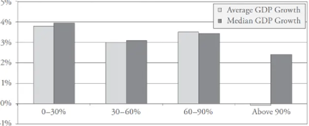
From the plethora of papers concerning such matters, the conclusions from Reinhart and Rogoff (2010) brought special attention to the idea of a debt threshold. This notion demarks a point after which debt causes severe penalties in terms of economic growth. They claim that there is a similar behavior between public debt and economic growth for any kind of country. But they go beyond that notion, and identify a deficit of 90% as the threshold after which growth rates start to decline significantly.
Fig. 2: Median and average economic growth at different levels of public debt
(Source: Reinhart and Rogoff (2010))
The graphic shown in Fig. 2 is taken directly from the aforementioned paper, and clearly illustrates the main point of their work. It’s notorious that surpassing a 90% debt level brings about an abrupt impact on average GDP growth.
5 While they presented their conclusions after an empirical study, many others followed in investigating the existence of this threshold through modeling. They divided their analysis in accordance to distinct situations of public debt ratios and from there drew conclusions in terms of average and median growth implications.
It’s not an overstatement to claim that the idea of an 80%-100% threshold became very close to turn into a stylized fact. Academics advocated this as an undisputed fact, and many of those involved in studies that shaped policymaking were undoubtedly influenced by this idea. In fact, many opinion pieces related to this idea ended up being written in newspapers such as The Financial Times, as well as in many others. Accounts of such references may be identified through their website (www.reinhartandrogoff.com/reviews/).
There are a few other papers that deserve to be mentioned when it comes to this line of thought. Checherita and Rother (2010) use a two-step GMM model (as many other did) in order to infer on this threshold, and consider the standard concave function. The concavity fully incorporates the idea that public debt promotes economic growth until a certain turning point. See Patillo et al. (2004) for evidence of a non-linear relation between debt and growth (although in this case they consider only external debt). It’s also noteworthy to mention that linear models do not usually present significant results (see Baglan and Yoldas (2012)). Schlarek (2004), stands as one of the very few that find a linear connection between debt and economic growth (in his case negative).
Checherita and Rother (2010) is one of the very few papers that study the threshold in the context of the European Union. In most cases, academics either consider OCDE countries, or simply use the ones which provide a bigger dataset. They consider 12 countries, over 1970-2011. Not only do they conclude on a 90%-100% threshold, but they also ponder on the channels through which public debt affects the economy. However, their model does not allow for direct implications, and they end up modeling these channels separately. They find further evidence of a non-linear relation in the channels’ analysis. This paper ends up being a good summary of what the debt literature was until a certain point. Even the channels that they considered are the ones that were commonly mentioned on the debt literature. These include Total Factor Productivity (TFP) and capital formation (see Patillo et al. (2004) for both), as well as interest rates. Checherita and Rother (2012) suggest that the negative effects may start to manifest at an earlier 70%-80% threshold, this time also calling attention to the
6 importance of public investment and private saving. As is usual in debt literature, they incorporate measures to deal with questions such as endogeneity (debt affecting growth, while growth also affects debt). The standard solution is to use lagged terms. The common GMM allows deal with this issue with relative ease. None of them consider, however, questions of heterogeneity.
Many others approached a similar line of study, trying to find covariates that closely related with the relation between public debt and economic growth. Ceccheti et al. (2011) is an example of a paper that reinforces the concept of a 90% threshold. Another standard example is Kumar and Woo (2010). They infer increasingly larger negative effects from higher public debt, with repercussions in both investment and labor productivity growth.
It’s important to keep in mind that all these studies try to discern a tipping point that is common across various countries. This is a consequence of the idea that economic growth and debt behave similarly across countries. Furthermore, the models used usually stick to investigating this threshold; as such, no direct implications are drawn in terms of channels, adding a layer of complexity when it comes to drawing conclusions viable to be applied in policymaking.
Another idea that molded the debt literature predates the Reinhart and Rogoff (2010) contribution – the notion of debt overhang (Krugman, 1988). The main idea is that a high external debt will cause most of a countries’ generated growth to be diverted to foreign countries. This notion has clear implications in the desire to invest and in economic growth itself. Many of the older papers that dealt with the study of public debt considered only the external aspect of it. This is the main reason why any kind of tipping point mentioned in older papers usually presents such a discrepancy when compared to much more recent literature.
The notion that we may have a common tipping point is a tempting idea: after all, it brings forth implications that help guide modern policymakers. However, there are aspects that should be taken into account and not relegated to a second plane. It’s ever more debatable how exactly to deal with the implications provided, as is questionable by many whether such a relationship exists at all.
It’s interesting to denote that the very same paper that inspired such a heated debate in a certain direction was also the paper that created a distinct standing point in the growth-debt debate. Herndon et all (2013) tried to duplicate the results obtained by Reinhart and Rogoff (2010). Their conclusions questioned the stylized-fact-to-be in
7 such a manner, that the entire debt literature focused instead on determining whether there is or not solid evidence that public debt as a relevant impact in terms of economic growth.
Herndon et al (2013) concluded that errors in the way the debt variables were weighted, along with errors in processing information caused severe inaccuracies in their conclusions. Their paper largely contradicted the severe difference in economic growth when below and above the 90% threshold. Even the database used presented limitations, with excluded data and gaps. These exclusions ended up having a severe impact in their conclusions. Herndon et al. conclude that this tipping point will only start to happen at a larger interval (when debt tends to 120%, and even then not as abruptly as expected). Considering the impact that the idea of a 90% threshold had until then in both academics and policymaking, it’s not hard to comprehend the consequences in terms of economic analyses. All of the studies that followed this notion ended up being called into question, as it became clear that the 90% threshold was not, after all, a “well-known stylized fact”.
There are also other aspects that must be taken into account. The common IV estimators, as well as the GMM model present limitations not only in the kind of information they provide, but also in their application. The coefficients drawn from the GMM models ended up being similar to the inadequate OLS (which can be seen through the tables in Kumar and Woo (2010)). Not only that, but this model is not ready to deal with the kind of databases that usually are considered in this kind of literature (due to weak instruments; see Bond (2012)). Normally, it’s considered a panel data methodology with too few covariates. In fact, the available data usually dictates that we are incapable of using as many variables as we may like, due to lack of enough years of observations. Furthermore, while most papers consider a time spam of around 40 years, the fact stands that most countries do not possess this kind of data currently available. As for the cases where this lack of data does not occur, it would still be desirable to obtain a much larger amount of data. This may well be the main reason why it is so difficult to find papers that address these questions in the context of the European Union. This fact is especially notorious if we consider the countries that joined the EU after the “original” 15. For these countries, most variables present around 20 years of observations.
As already mentioned, there were also those who highly started to question whether there was in fact any evidence that supported the existence of a relevant
8 threshold. This created an interesting phenomenon, in which the absence of significant results is a significant academic contribution in itself. Prime examples of this trend are works such as Pescatori et al. (2014) and Eberhardt and Presbitero (2013), in which there is absolutely no evidence of a magical, well-defined threshold. Pescatori et al. find, however, that a higher debt level implies a higher level of output volatility. As for Eberthardt and Presbitero, they conclude upon the nonlinearity between debt and growth. Both conclusions point to the hypothesis that there is still room to innovate when it comes to the relation between both variables, and therefore draw conclusions that prove themselves relevant in terms of policymaking.
The already mentioned paper of Eberhardt and Presbitero (2014) summarizes one of the most pressing matters in terms of what is now expected in terms of debt literature contribution. They conclude that there are no common thresholds across countries. This idea brings us to that which is the one of the main flaws on recent debt-related studies. The existence of a common tipping point as an appropriate rule of thumb is appealing to any policymaker. However, both its veracity and utility are easily put into question. After all, the determinants of any country’s public debt are numerous. Furthermore, they will be distinct across countries. As such, the idea of a common threshold is an unfeasible notion. Unless there is a convergence such in terms of policymaking that draws the debt-structures across distinct countries together, we cannot abide by such a stringent concept.
Another limitation that must be addressed is the lack of conclusions in terms of channels through which public debt affects (or nor) economic growth. Through such information, policymakers should be able understand which debt components may be used as a mechanism. Not just as a way to control high debt levels in times of crisis, but also to properly use public debt as intended – as a tool that allows for economic growth.
A recent paper released by Lin (2014) presents distinct contributions that represent a big first step in addressing such questions.
Lin uses an adaptive Lasso quantile regression model. This has an immense number of contributions to the current state of debt literature. First of all, the fact that he considers quantile regression allows us to infer on many different scenarios all at once. That is to say that whether a given economy is performing as expected, below or above predicted values, we may be able to infer which debt components may be used as a proper mechanism for policy implementation. Such information would obviously be invaluable.
9 Furthermore, the adaptive Lasso allows for a very high number of covariates to explain growth. That is to say that we may consider a rather ample number of channels – since public debt may have a diverse number of components this is certainly an invaluable characteristic. Usually, the limited number of observations dictates that a reduced number of channels must be considered. The Lasso, however, allows for a high number of covariates to be included, while ensuring stability of the model (see Zheng et al (2013)). By combining this aspect with the information that result directly from Quantile Regression derives useful and detailed information in regards to channels and their application in policymaking. In that sense alone, this sort of model is a clear contribution to the debt literature.
One of Lin’s main contributions in terms of conclusions is precisely what he derives in terms of channels-related conclusions. He states that there seems to be a certain divergence between the relevant channels for both developed and developing countries. Developed countries should focus mainly in questions such as monetary policies and capital investment. For developing countries, factors such as infrastructure investments and demographic factors are the most important factors. These conclusions are in line with what is logically expected; it’s quite understandable that these kinds of factors affect much more countries that are in an earlier development state than richer ones.
Lin advocates that these thresholds will have a wide variance across countries – between 10% and 100%. Even if we are to question these values, we cannot disregard its importance, for they help to help to question the adequacy of the common threshold concept.
Lin’s contribution served as the main methodological basis for the development of this dissertation.
10
3. Economic Theory on Debt
Before discussing the details of the model, we must ponder about the nature of public debt. After all, it’s important to understand why it serves as an extremely important part of policymaking.
Governments try to ensure that the essential sectors of the country work as they should. By impacting education, health, justice, and others, they impact their countries as well. In some cases, by creating or managing public institutions, they affect some markets and branches of activity. As an example, the Portuguese government has a public bank, namely Caixa Geral de Depósitos.
By their nature, however, governments are supposed to ensure that any activities that are included within their sphere of competences are working properly at all times. Due to economic fluctuations, the required means necessary to do so may not be always available. As such, acquiring such funds becomes a vital necessity.
Public debt, as a broader concept, measures an obligation that a certain central government has to a lender (internal or external). It results from the necessity of ensuring that a governments’ duty is performed, since they usually operate within the central aspects of a country’s management.
Knowing this, it’s quite easy to understand how public debt acts as an attractive short-term solution. Since this is often realized through the emission of bonds, it’s quite easy to get a hold of investors that seek reliable investment opportunities. But this attractiveness, along with the ease to access easy funds, may easily backfire. These characteristics imply that there is a tendency to acquire further funds to promote a government’s ability to impact its country. As a result, government deficits usually grow over time. In Europe, for example, the data clearly shows that as a norm, countries augmented their public debt/GDP ratio quite significantly over time.
This brings about a serious long-term management problem, compromising a country’s development in the long-run. As such, it is important to understand the limits of this tool. This idea brings us to the notion of sustainability. It’s necessary to infer on the limit between a solid funding decision and forcing an inadequate level of investment. Governments need ever more to be able to identify the tenuous point that separates these two situations.
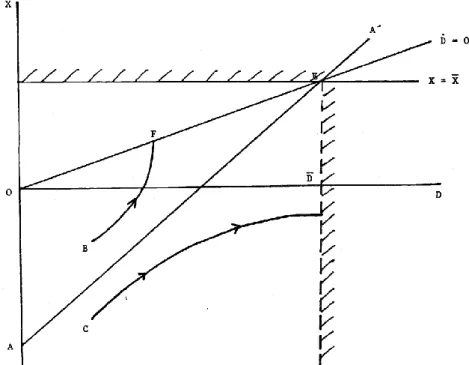
11 Blanchard (1984), is a good example on the first approaches to this very question, presenting a simplified model to define sustainability, while pondering on the role of fiscal policy. In these cases, public debt would be sustainable as long as:
(1)
In this equation, r corresponds to the real interest rate. Interest rates are a very important notion in debt literature, since it closely determines the cost of debt contraction. Inflation appears then as a possible tool. Monetization, as is widely known, has been a solution employed in cases of utmost necessity, although usually at a great cost, namely hyperinflation.
The variable D measures government debt. Beyond D , the government would be unable halt the increase of public debt.
The variable X measures a budget surplus/deficit (depending on whether X is higher or lower than 0) at a given time. As for , it reflects the maximum achievable surplus. The difference between the two could be diminished at a given rate α. The following image (Fig. 3) depicts the model.
12 The representation allows us to differentiate between sustainable and unsustainable scenarios.
Point E represents a situation in which a government achieved a maximum surplus through the maximum sustainable debt level D . Desirably, the growth rate of X ( ) surpasses the growth of D ( ) at all times. Therefore, points above AE reflect the sustainable and appropriate debt contraction scenarios.
While simplistic, the model does a decent job at representing the most basic concepts on debt as a tool for growth.
The IMF, as an international economic organization, releases a multitude of documentation regarding these ideas. Escolano (2010) presents a compilation of formulas that concern different aspects of the role of public debt. Amongst the various aspects considered, he includes a formula for debt sustainability as well.
(2)
Nominal GDP growth rate is here given by γt,, while yt measures the real GDP at
t. As for it, it reflects the nominal interest rate. A no-Ponzi game rule is incorporated,
due to the possibility of λ>0. As such, creating further debt to deal with the existent one is not an admissible strategy. This derives from cases where it constantly surpasses γt
and the debt escalates. As for D0, it represents the initial debt level. Finally, pt represents
the primary balances at a given t.
This sustainability formula derives directly from the government budget constraint, by replacing the variable pt with a (pt + st):
(3)
This expression means that all incoming primary balances must allow the repayment of the initial debt, along with the resulting interest.
Therefore, a certain level of debt will be sustainable as long as the government budget constraint is ensured. In cases where the government intends to contract further debt, the variable S in the former equation measures the difference that occurs between the sum of the future primary balances and the debt that must be paid. The larger this
13 amount increases, the more difficult it is to ensure that the budget constraint is satisfied. This is how the variable measures the consequences of contracting high deficits.
4. Data and Methodology
4.1 Data
The database used in this dissertation contains information regarding the countries of the EU-15. The amount of observations for each country varies between 41-48 observations. The tables presented in the annexes indicate the time span considered for each country. Unfortunately, while this amount of observations is in accordance with the recent literature, it is also far from what would be desirable for this sort of analysis.
Due to limitations of the model estimation, which will be discussed in the following chapter, I considered mainly economic variables. This assortment is largely inspired by the Lin (2014). Even disregarding such restrictions, the poor availability of data means that it is quite unfeasible to find a common set of variables for all countries. When considering non-economic variables, it is quite common that at least a third of the countries considered do not have sufficient information.
Sources such as the IMF database consider only information from 1980. When it comes to obtaining data prior to this point, information tends to be scarcer. This implies that information must be gathered from various sources.
Debt literature is overall quite dependent on large data samples. All these shortcomings are the reason that makes any king of debt analysis in the EU uncommon. The standard practice is to consider whatever group of countries offers the most adequate set of data. This is why most papers consider countries from the OECD.
The main source of data was the World Bank website. They offer the most complete amount of data possible. In cases where the data offered was insufficient, further information was extracted from the AMECO database, as well as the IMF and OECD websites. The debt/GDP ratios were mainly taken from the data used by Reinhart and Rogoff. This data is easily accessible through their website.
14
g - GDP per capita growth rate (Worldbank, IMF)
Debt – general government gross debt to GDP ratios (Reinhart e Rogoff, AMECO,
OECD, IMF)
EMU - Dummy for the countries that belong to the Economic and Monetary Union. In
the EU-15, only Denmark, Sweden and UK refused to join the Euro
Openness - measures a country’s openness to foreign economies; obtained through the
sum of exports and imports (as a percentage of GDP) (WorldBank)
Unemployment - Unemployment rates (AMECO, IMF). Not enough data was available
for Germany, and it was therefore excluded in that particular case
TaxRevenue - tax revenue as a percentage of GDP (OECD) Inflation - inflation rates at consumer prices (WorldBank, IMF) Capital - Gross fixed capital formation (WorldBank)
Savings - Gross domestic savings (as a percentage of GDP) (WorldBank) PopGr - population growth rate (WorldBank)
NomIntRate - long-term bond-yields for France, Germany, Ireland, Italy, Spain and
UK (OECD); in cases where data was unavailable, the data for Germany was used as a benchmark
RealIntRate – the real interest rate was calculated through NomIntRate and Inflation
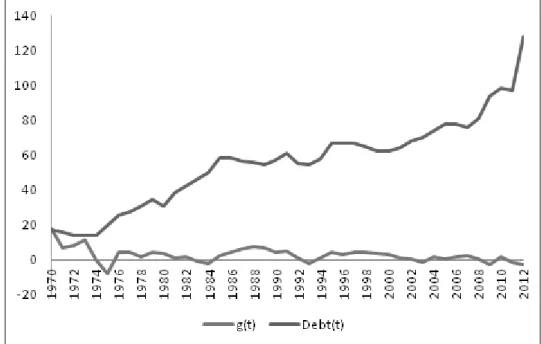
Before proceeding with the description of the methodology employed, let’s take a quick look at the data available for Portugal. The graphic presented in Fig. 4 represents the evolution of the GDP growth rate as well as changes in the debt-to-GDP ratio. Both variables are shown as percentages, and spam the period between 1970 and 2012.
The data suggests that, for the Portuguese case, debt contraction became a relevant policy around 1974-1975. As is well known, this period corresponds to a change in regime, and therefore to a change in policy implementation. This period also corresponds to the first oil crisis. Since then, the debt ratio presents a clear tendency to increase over time, particularly in the last few years of our sample. Conversely, as time passed and the public debt soared, the GDP growth rates show an increasing tendency to remain close to 0%. Curiously enough, this is especially notorious around 2001-2002, period marked by the implementation of the Euro as a currency.
15 Following the crisis in the 70’s and subsequent drop in oil prices in the 80’s, there seems to be a slowdown on the increase of public debt. This corresponds to a decreasing GDP growth rate until 1984
In the 90’s, likely due to the Maastricht treaty (signed in the beginning of 1992), the debt level stays relatively close to a 60% of GDP. It is also noteworthy that while there was a recession in the early 90’s, the same period presents an increase in public debt, until 1992.
Around the year 2000, there was a small yet clear attempt to converge the debt levels to 60% of GDP, as per the criteria included in the aforementioned treaty.
4.2 Methodology
As previously stated, this dissertation is largely based the contribution by Lin (2014). His main contribution is the Lasso estimator for Quantile Regression models. The growth-debt model is simply an application. That is to say that Lin’s contribution is mainly in terms of methodology, not in terms of results. In comparison, the presented dissertation offers much more detailed results, allowing for more in terms of analysis and conclusions regarding the subject.
Fig. 4: The evolution of the Portuguese public debt (% GDP) and GDP growth
16 Unlike Lin, however, I did not include the Lasso estimation for the main model. This choice derives from the computational requirements that such a methodology implies. As a result, the number of variables that I consider must be smaller. It is noteworthy to mention that despite using the Lasso to allow the use of a huge amount of variables, Lin´s results still present many cases in which a threshold is not identified. While it may be argued that this simply indicates a lack of a proper threshold for those particular cases, it may also derive from the sheer amount of variables included. Even with the Lasso, the strain of an exaggerated number of variables is bound to impact negatively the results. Also, while Lin ended up using a different set of variables for each country (due to the data shortcomings), this does not happen in mine.
I use a threshold Quantile Regression model. This kind of model has a few implications in regards to the way we analyze the effects on debt on growth. The idea is that the model gives information in accordance to the levels of gt. This means the
appropriate debt threshold (and respective channels) is dependent on the way the considered economy is performing. It’s quite easy to understand how these kinds of implications are relevant; they hint at possible policy-making decisions in times of crisis or even economic expansion.
Egert (2013a, 2013b) and Eberhardt and Presbitero (2013) were already mentioned for contesting the idea of a common threshold between countries. They claimed that allowing for heterogeneity across countries rendered the results irrelevant. See their papers for more detailed information. As it happens, this model allows heterogeneity, since we are using a time series model (uncommon in this strand of literature). Most of the debt literature that tries to find a common tipping point fails to even address this question.
The model follows the equation:
(4)
As shown in the variables list, gt represents the GDP growth rate of a given
country at time t. As for Xt, it encompasses the remaining variables (our covariates).
The last term consists on an intersection between the covariates and a dummy that represents any instances where debt surpasses a given debt threshold. I(z) corresponds to an indicator function that will take the value of 1 if z (in this case (DEBTt-1 > γ(τ)) is true. Keep in mind that γ(τ) corresponds to a given debt level that is
17 being taken into consideration for a certain τ (quantile). The debt term corresponds to the lagged debt-to-GDP ratio.
This last term analyzes the impact of surpassing the most adequate debt level through a given covariate (by other words, the channels). By finding this , we infer on the effects of an exaggerated debt level on growth through a given channel. These are measured through the coefficients β’(τ) and δ’(τ).
I propose using a two-step estimation approach, which is standard in threshold models. For each τ, we define a grid for the admissible range of values for γ. The Quantile Regression estimator is applied for each and every possible value of γ. The one with the highest fit is to be considered the final point estimator, . From that, we obtain the correspondent and , which in fact are and
As a side note, we used the Bofinger bandwidth estimation method to obtain the coefficients’ standard errors. In an earlier development stage of the model, this method appeared to perform better with a higher number of covariates. There are multiple ways to perform this sort of estimation, while there is no consensual optimal option. Therefore, it is simply a small modeling decision without any kind of negative implications.
5. Main Results
The presented model is able to determine the adequate threshold and relevant channels for every τ in every country, disregarding very few exceptions. These few cases are situations in which the model, despite proposing a certain threshold as optimal does not present any statistically relevant channel or impact on gt through the dummy
DEBTt-1 itself. All the results were obtained through the EViews software.
The annexes present all the relevant information in detailed tables for each country. These include the amount of observations, estimated threshold, relevant channels, and respective coefficients. The following table summarizes the obtained results, and contains only the cases in which relevant thresholds are presented. In the annexes, irrelevant thresholds were included, since they are still provided from the model.
18 τ = 0.1 τ = 0.25 τ = 0.5 τ = 0.75 τ = 0.9 Austria 67 67 38-39 34-35 34-35 Belgium 66-74 66-74 97-98 --- 96 Denmark 7 7 42-45 42-45 42-45 Finland 23-39 23-39 23-39 9-10 9-10 France 22-24 22-24 34-35 34-35 34-35 Germany 63-65 63-65 28 28 28 Greece 34-40 34-40 30-33 66-89 66-89 Ireland 65 65 70 63 65 Italy 49-50 51-53 51-53 36-38 36-38 Luxembourg 7 15 15 --- 10 Netherlands 65-67 65-67 65-67 50-51 --- Portugal 56 67 35-38 35-38 35-38 Spain 17-20 44-45 46 42 42 Sweden 48 48 26 26 26 UK 50-51 --- 43 47 50
Table 1: Estimated thresholds for each member of the EU-15 per quantile
It’s extremely interesting to note that with the exception of Belgium at the top quantile, no country presents an insanely high debt as adequate. Even then, the suggested threshold does not surpass 100% GDP. This may be an indicator that countries should not overreach when it comes to contracting debt, even if the desired effect is to invest and boost economic performance. This conclusion is especially important if we compare the results with any paper that advocates a threshold of 90% across countries.
Cases where the significant thresholds are presented as an interval result from scenarios where the results are identical across all possible γ in that interval. It’s likely that these result from situations in which there were large debt contractions. As an example, let’s consider Greece. For τ=0.75 and τ=0.9, we have an optimal γ* between
19 66% and 89%. When looking at the data, it’s possible to identify a big debt growth from 65.8 to 89.1. This example serves also to show how much this sort of analysis depends on available data.
It’s quite interesting to note that there is usually some sort of stability between different quantiles in a given country. The fact that a country is able to have a certain similarity between multiple quantiles has pleasant policy implications, since it indicates a relative stability in the desired thresholds. Cases such as France or Germany are a prime example of this. There is a clear distinction between only two different thresholds across all τ. The fact that multiple quantiles can point to the same γ only gives the appointed threshold a higher level of credibility. This type of study usually serves to provide guidelines on how to manage public debt. Thus, having a tipping point associated with various cases in which the economy is performing similarly implies that the considered γ serves as an appropriate rule of thumb.
Another very interesting aspect is the way we perceive the necessity of debt contraction. While it is true that some countries present higher optimal debt levels in lower-performing scenarios (τ=0.1, τ=0.25), such as Germany or Portugal, this is not always the case. Denmark and France appear as clear cases where public debt should instead be contained in cases of under-performance.
In order to understand the contribution of the model, let’s see some specific examples. Let’s analyze the information that the model offers in terms of channels through which debt may or may not affect debt. I will analyze the cases of Germany, Greece, Portugal and UK, since they are some of the most interesting cases.
Tables with the relevant information are provided for each of these countries. They detail the coefficients of the relevant covariates for each quantile. These regressors include the dummy DEBTt-1>γ along with the potential channels. Note that the
remaining variables correspond to the last term of the equation δ1 (τ )Xt I (DEBTt-1 >
γ0(τ)). In other words, the coefficients presented represent the effects they cause on
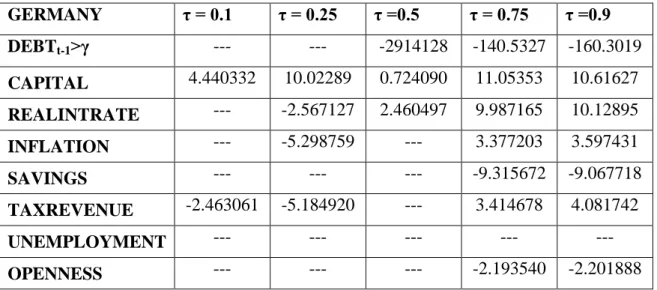
20 GERMANY τ = 0.1 τ = 0.25 τ =0.5 τ = 0.75 τ =0.9 DEBTt-1>γ --- --- -2914128 -140.5327 -160.3019 CAPITAL 4.440332 10.02289 0.724090 11.05353 10.61627 REALINTRATE --- -2.567127 2.460497 9.987165 10.12895 INFLATION --- -5.298759 --- 3.377203 3.597431 SAVINGS --- --- --- -9.315672 -9.067718 TAXREVENUE -2.463061 -5.184920 --- 3.414678 4.081742 UNEMPLOYMENT --- --- --- --- --- OPENNESS --- --- --- -2.193540 -2.201888
Table 2: The German case - Estimated coefficients of the relevant channels at the
considered threshold
We can see that public debt affects the German economy through a higher variety of channels at times of economic expansion.
It’s notorious that in Germany’s case, simply having a debt threshold beyond the optimal amount has a negative impact on the growth rate. This becomes especially evident when considering a scenario in which the economy is performing exceptionally well. This happens for the cases in which =28%.
Capital formation stands out as the most relevant channel, since it appears as a relevant channel independently of the way gt behaves. We can see that augmenting debt
beyond the recommended level still allows for a positive effect for economic growth through capital formation. It appears to have a smaller relevance when τ =0.5. It seems that in Germany’s case, capital formation appears as a strong source of economic growth, even if we decide to accept an exaggerated level of debt.
In cases where the economy is performing poorly, the real interest rates seem to be depreciative to economic growth. Financing investment will be more expensive. The negative value reflects the idea that a government should not try to force investment through acquiring extra funds. This situation changes as the economy performs better. By other words, investment is still a relevant source of growth as long as the economy is performing well.
As for inflation, it presents a positive value as long as we have a favorable growth. This may be due to the fact that salary increases are more likely to match
21 inflation during a time of expansion. Therefore, public workers whose activity is likely to be supported through debt contraction, are in better position to either save up and invest or consume and incentive business dynamics. Inflation, in debt literature is well associated with money supply. Monetizing debt, an approach used by many countries (not allowed anymore for countries with the Euro) usually resulted in an adverse effect on economic performance. This may be the reason why it shows a negative impact in a case of poor economic growth. Unable to repay existing debt through wealth creation, debt monetization could have been an answer at some point in time. Do remember that our sample includes observations prior to the adoption Euro.
It’s quite interesting to see that savings become a hindrance to the economy in times of growth. The values indicate that consumers have an incentive to consume various goods and services. This idea makes sense if we consider that is a standard practice to detain public companies in a few select markets. Economic agents have then an incentive to consume these types of goods/services. Public debt may have been contracted in order to develop these kinds of institutions/companies. If we are in the upper distribution of gt, then consumption will allow these companies to outgrow the
debt cost.
The amount of taxation for τ = 0.1 e 0.25 clearly impact the economy negatively. Taxes are a standard short-term solution to counter an existing high level of debt. The negative values represent the economic cost that results from maintaining a high debt level. In cases where Germany is experiencing an economic boom, the debt incurred is more likely to result in wealth creation. This may well be the reason why taxation presents a positive value. This implies that the wealth generated from government intervention financed through debt contraction is higher than the cost of taking money away from the citizens. Therefore, the German government should maintain a more active role in the economic development in times of expansion. This conclusion also brings us to the idea that debt contraction is largely dependent on how effective investment is. It gives some credibility to the usage of debt as tool for growth, in the right hands and right conditions.
Finally, we have our trade indicator. Openness presents a detrimental effect once we incur on high debt levels. This may well result from an excess of imports. If the contracted debt served to boost public sectors, it becomes imperative that these make the investment generate as much wealth as possible. This may indicate severe inefficiencies in a given economy. Germany will likely rely on foreign economies to
22 cover for any market shortcomings of its own economy. Any percentage of the debt contracted that is dedicated to a case of severe foreign dependence such as this will likely result in very little wealth creation. This is likely the reason why the variable impacts the economy negatively.
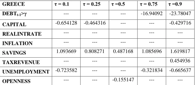
Let’s now check the Greek case.
GREECE τ = 0.1 τ = 0.25 τ =0.5 τ = 0.75 τ =0.9 DEBTt-1>γ --- --- --- -16.94092 -23.78047 CAPITAL -0.654128 -0.464316 --- --- -0.429716 REALINTRATE --- --- --- --- --- INFLATION --- --- --- --- --- SAVINGS 1.093669 0.808271 0.487168 1.085696 1.619817 TAXREVENUE --- --- --- --- 0.454936 UNEMPLOYMENT -0.723582 --- --- -0.321834 -0.665637 OPENNESS --- --- -0.155147 --- ---
Table 3: The Greek case - Estimated coefficients of the relevant channels at the
considered threshold
As it happened with Germany, simply contracting a huge debt level will lead to increasing negative effects in cases of economic expansion.
Capital formation appears as largely ineffective once we allow for a high level of debt. A quick glance at the information detailed in the annexes shows that, by itself (not as a channel), capital formation tends to generate economic growth. However, this variable will only show up for τ=0.1 and τ=0.25. Therefore, the data suggests that, in the Greek case, an abusive deficit leads to detrimental capital formation.
Savings appears as the most relevant channel, since it is relevant independently of economic performance. Furthermore, it presents a similar behavior in all cases. This may well imply that upon creation of debt, the Greek must strive to invest more in order to boost economic performance, and therefore allow the control of the debt incurred.
23 The amount of taxes collected in the top percentile has a positive impact, likely representing an externality caused by the economic boom. Better performance by the economy means more funds available to the consumer. This simply shows that enough income is generated to properly fund public debt.
Unemployment acts detrimentally across different economic scenarios, and may imply that either the Greek labor market or the subsidy systems were characterized by severe limitations. Part of the contracted debt may have been directed towards subsidies, posing a significant cost.
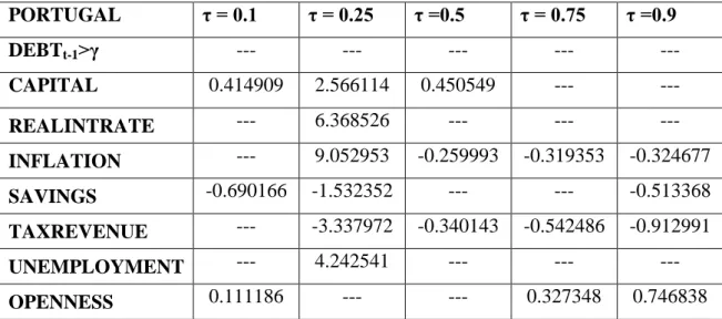
For the Portuguese case:
PORTUGAL τ = 0.1 τ = 0.25 τ =0.5 τ = 0.75 τ =0.9 DEBTt-1>γ --- --- --- --- --- CAPITAL 0.414909 2.566114 0.450549 --- --- REALINTRATE --- 6.368526 --- --- --- INFLATION --- 9.052953 -0.259993 -0.319353 -0.324677 SAVINGS -0.690166 -1.532352 --- --- -0.513368 TAXREVENUE --- -3.337972 -0.340143 -0.542486 -0.912991 UNEMPLOYMENT --- 4.242541 --- --- --- OPENNESS 0.111186 --- --- 0.327348 0.746838
Table 4: The Portuguese case - Estimated coefficients of the relevant channels at the
considered threshold
Unlike the previous cases, there are no direct implications that result from sustaining an abusive debt level.
Furthermore, capital formation still performs well under duress, as it still bolsters the economy under economic retraction.
As a channel, inflation presents an opposite behavior to the German case. With higher inflation, consumption and costs overall rise. Unlike Germany, we had a weak currency prior to the Euro. Such an aspect has direct implications in regards to external debt accumulation. In order to improve economic performance, we incurred at a cost that contracted the positive effects of an economic expansion. However, at τ=0.25,
24 inflation detains a positive effect, implying that investment was necessary even if it meant contracting debt at a higher cost.
For the Portuguese case, this is where it gets interesting. In distinct economic performances, both the funding that results from taxes and the accumulation of savings have a detrimental effect upon abusive debt incurrence. In terms of policy, it suggests that if we wish to boost our economic performance while maintaining an exaggerated level of debt, then there must be as many incentives as possible to private consumption. It also seems that the Portuguese balance of trade benefits by incurring on extra debt. Chances are that a part of the contracted debt serves to fuel relevant internationally competitive economic sectors.
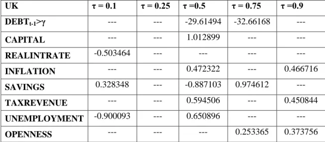
Finally, a quick look at the results obtained from the United Kingdom.
UK τ = 0.1 τ = 0.25 τ =0.5 τ = 0.75 τ =0.9 DEBTt-1>γ --- --- -29.61494 -32.66168 --- CAPITAL --- --- 1.012899 --- --- REALINTRATE -0.503464 --- --- --- --- INFLATION --- --- 0.472322 --- 0.466716 SAVINGS 0.328348 --- -0.887103 0.974612 --- TAXREVENUE --- --- 0.594506 --- 0.450844 UNEMPLOYMENT -0.900093 --- 0.650896 --- --- OPENNESS --- --- --- 0.253365 0.373756
Table 5: The British case - Estimated coefficients of the relevant channels at the
considered threshold
The most obvious aspect here is the lack of relevant channels for τ=0.25. Therefore, the threshold appointed by the model is irrelevant. This was one of the very few cases in which this occurred. At any rate, my model offers more information on optimal γ than what can be seen in Lin(2014).
As it was with both Greece and Germany, excessive debt has direct negative implications on growth.
25 Similar to the German case, inflation appears as beneficial in ths type of situation. Therefore, the same principle may apply.
In the UK case, the savings appears to have a rather unique behavior, only being detrimental for the median values of gt. In cases of extremely low economic
performance, however, as long as the UK maintains an excessive amount of public debt, there appears to be a clear incentive to allow for savings accumulation. This may well reflect the characteristics of private investment within the country.
As for income that may derive from the extra taxation, it seems that in cases where the economy is not performing poorly, this will not be a problematic aspect of the British economy.
The data regarding the unemployment in the country suggests that only under economic duress will there be a need to divert a significant amount of the incurred debt towards subsidies. This will likely be the reason why it affects the counry negatively for τ=0.1. For τ=0.5, however, the data suggests that funds made available to the unemployed have a positive effect through consumption. Interestingly enough, for the same τ, savings presented a negative value.
Finally, it seems that when it comes to international trade, UK and Portugal present a similar behavior. During an expansion, part of the extra debt incurred will likely be destined to relevant competitive economic sectors.
For the remaining countries, see the information contained in the annexes.
6. Future Research
Due to the nature of this strand of literature, there is a very large room for improvements and new findings. As we strive ever more to improve policymaking decisions, we must be able to keep evolving in the way we model and analyze public debt. For now, considering the many limitations still present in this kind of research still fall short of what is required.
While not a new area of research, it is vital to understand the following aspect. The dependency on available data characterizes this line of work on a very significant level. It is therefore necessary to augment our sample size and redo this kind of estimation on a regular basis. In time, this will allow us to include a wider range of
26 variables to great effect. The sheer improvement in the results resulting from such a supposedly small idea would be immense.
One of the main limitations in terms of analysis derives from the fact that I developed a static model. The model properly identifies the optimal debt thresholds along with their respective channels. But economic performance is ever changing. It’s true that, overall, countries present multiple τ with identical thresholds. It’s also true that there is no threshold that holds for all τ in a given country.
As economic cycles occur, policymakers that wished to abide by the guidelines provided in this dissertation would still have to worry about transition dynamics. This is why I advocate that the development of a dynamic version of this model will be an upheaval on this kind of analysis. The requirements for such a model would be immense, both in data and theoretical knowledge. This kind of analysis should be taken into account as one of the ultimate goals in studies regarding public debt.
By looking at the Greek data, we can easily comprehend why this question is so pressing. If we consider that Greece has a clear incentive to contract further debt in times of prosperity, then we must consider as well what happens should a recession follow. In such a scenario, Greece would be in a difficult position to reposition itself the appropriate debt level once more.
It’s also worth mentioning that while my model is perfectly capable of identifying the most adequate threshold for each τ, it completely disregards the remaining results. This implies that, should there be any cases where there are thresholds nearly as adequate, we will never be aware of them. Another relevant aspect is that the model says nothing about debt thresholds in vicinity of the indicated one. Even if we claim that a country should strive to maintain a debt of 50% of GDP, government stabilization efforts will likely result, at most, in a 48%-52% interval, or similar. Therefore, this kind of information is also of extremely relevance.
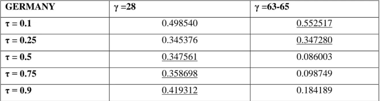
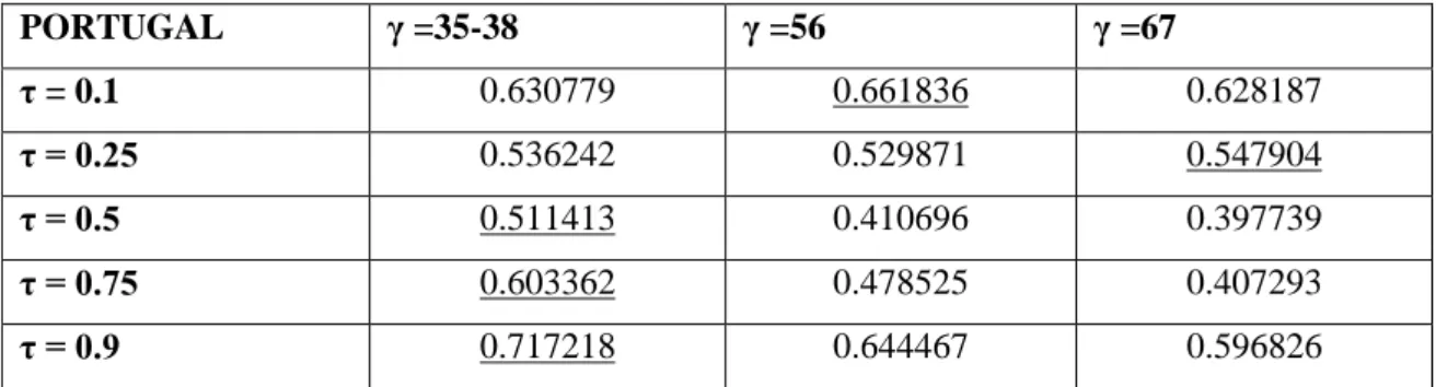
I present two very interesting cases. Both represent well the costs of information loss. In both of them, this kind of information would allow to maintain the same γ across all quartiles. I consider namely Germany and Portugal.
27 GERMANY γ =28 γ =63-65 τ = 0.1 0.498540 0.552517 τ = 0.25 0.345376 0.347280 τ = 0.5 0.347561 0.086003 τ = 0.75 0.358698 0.098749 τ = 0.9 0.419312 0.184189
Table 6: The German case – comparison between relevant thresholds across all
quantiles
The underlined values indicate which of the γ is optimal for each instance. But what the standard model usually does not show is that, for cases where the German economy is not performing well, γ=28 appears as the second most adequate level of debt. As can be seen by the adjusted R2, the performance would be nearly as optimal as the suggested 63-65. And why exactly is this so interesting? Because γ=28 corresponds to the optimal level when the economy is not performing poorly.
As a result, if we were to consider such a result in a dynamic process, 28% would be taken into account as the optimal debt level. By doing this kind of differentiation, we would avoid the costs and complications that derive from the transition from one optimal state to another. It’s also easy to note that the opposite does not hold; a debt level between 63% and 65% does not maintain a stable performance across all quantiles. This is shown by the low associated R2 for τ=0.5, 0.75 and 0.9. Accepting this threshold level for cases of low economic performance only would imply a constant transition from one debt level to another. Augmenting the debt levels in accordance to this information would seem easy when transitioning from a γ=28 to a γ=63-65. We must not forget, however, that once the economic situation reversed we would be left with a difficult endeavor to reduce public debt levels once more. This fact further relays the idea that the transition dynamics have an extremely important role when accounting for public debt.