Public Debt and Economic Growth: a Granger Causality Panel Data Approach

(1)

Carlos Pestana Barros & Nicolas Peypoch

A Comparative Analysis of Productivity Change in Italian and Portuguese Airports

WP 006/2007/DE _________________________________________________________

Cândida Ferreira

Public Debt and Economic Growth: a Granger Causality

Panel Data Approach

WP 24/2009/DE/UECE _________________________________________________________

Department of Economics

W

ORKING

P

APERS

ISSN Nº0874-4548

School of Economics and Management

(2)

Public Debt and Economic Growth: a Granger Causality Panel Data Approach

Cândida Ferreira

ISEG-UTL

Instituto Superior de Economia e Gestão - Technical University of Lisbon - (ISEG-UTL)

and Unidade de Estudos para a Complexidade e Economia (UECE)

Rua Miguel Lupi, 20, 1249-078 - LISBOA, PORTUGAL

tel: +351 21 392 58 00

fax: +351 21 397 41 53

e-mail :candidaf@iseg.utl.pt

Abstract

This paper analyses the Granger-causality relationship between the growth of the real

GDP per capita and the public debt, here represented by the ratio of the current primary

surplus/GDP and the ratio of the gross Government debt/GDP.

Using OECD annual data for 20 countries between 1988 and 2001, we adapt the

methodology recently applied by Erdil and Yetkiner (2008) and we conclude that there

is clear Granger causality and that it is always bi-directional. In addition, our findings

point to a heterogeneous behaviour across the different countries.

These results have important policy implications since not only does public debt restrain

economic growth, but also real GDP per capita growth influences the evolution of

public debt.

JEL classification: C23; C12; H6

(3)

Public Debt and Economic Growth: a Granger Causality Panel Data Approach

1. Introduction

The relevance of the public debt to economic growth has become crucial, particularly to those

policy-makers who nowadays have to face increasing fiscal imbalances.

In terms of economic theory, it is widely accepted that at moderate levels of public debt, fiscal

policy may induce economic growth, with a typical Keynesian behaviour, but at high public

debt levels, the expected tax increases will reduce the positive results of public spending,

decreasing the investment and consumption expenses, with less employment and lower GDP

growth rates.

On the other hand, there is a broad consensus view that lower GDP growth may also be

synonymous with less public revenue and sometimes more public expenditure in social

security transfers and other subsidies paid by the Government, which can contribute to the

increase of public debt.

However, little empirical investigation has been conducted into the link between public debt

and economic growth and the obtained results are still rather inconclusive.

Some authors, like Modigliani (1961), Diamond (1965) or Saint-Paul (1992), have suggested

that an increase in the public debt will always decrease the growth rate of the economy.

Recently, several theoretical and empirical works analyse the relationship between the external

(and not specifically public) debt and economic growth in developing countries.

Patillo et al. (2002 and 2004) conclude that at low levels, total external debt affects economic

growth positively, while at high levels, this relationship becomes negative. Presbitero (2005)

uses dynamic panel estimations and find a clear negative relationship between external debt

(4)

Schclarek (2004) uses a panel including 59 developing and 24 industrialised countries. For the

developing countries, he concludes that there is always a negative and significant relationship

between total external debt and economic growth, in clear contrast with the results obtained by

Patillo et al. (2002 and 2004), while for Schclarek (2004), there is no evidence of a positive

relationship between total external debt and growth at low debt levels. In the case of industrial

countries, Schclarek (2004) does not find any robust relationship between gross government

debt and economic growth, suggesting that for these more developed countries, higher public

debt levels are not necessarily associated with lower GDP growth rates.

Perroti (2002) had already concluded that fiscal consolidations are more likely to have

non-Keynesian effects in countries with high debt levels. Furthermore, the European Commission

(2003) verifies that during the past three decades, only half of the fiscal consolidation episodes

in EU countries were followed by an immediate acceleration in economic growth. For some

specific countries in the EU (namely the cohesion countries), Mehrotra and Peltonen (2005)

find that an improvement in the net lending position of the government, as well as a fall in the

level of public debt, would be beneficial for socio-economic development in the medium term.

With this paper, we seek to contribute to the analysis of the Granger-causality relationship

between real GDP per capita and public debt.

We follow a panel data approach, adapting the methodology proposed by Hurlin and Vernet

(2001) and Hurlin (2004) and recently applied by Erdil and Yetkiner (2008) to analyse the

relationship between real per-capita GDP and per-capita health care expenditure.

Our findings point not only to the existence of Granger-causality between GDP per capita and

public debt, but also to the bi-directional character of this causality. In addition, we conclude

that there is heterogeneity among the OECD countries. They not only face different initial

conditions, but each country may also reveal distinct reactions, on the one hand, of economic

(5)

The remainder of the paper is organised as follows: we present the methodological framework

in the next section. In Section 3, we report the data used and the estimation results. Section 4

raises policy implications and draws some conclusions.

2. The methodological framework

The choice of methodologies to test Granger-causality with a panel data approach is not very

wide.

Most works in this field test vector auto-regression coefficient (VAR) panel data models

following the methods proposed by Holtz-Eakin et al. (1985, 1988), Weinhold (1996) and

Nair-Reichert and Weinhold (2001). These works mainly test cross-sectional linear restrictions

on the coefficients of the model, which are supposed to be variable.

Our methodology is an adaptation of the Granger-causality panel data approach with fixed

coefficients which was proposed by Hurlin and Vernet (2001) and Hurlin (2004) and recently

applied by Erdil and Yetkiner (2008). It relies on the use of F (or Wald) tests to analyse the

existence of causality among the variables.

We also follow Konya’s (2004) concerns over unit-root tests. Thus, we first test the stationarity

of the variables, using the Levin, Lin and Chu (2002) test and, according to the obtained

results, we then choose to use the variables either in levels or in first differences.

The use of panel data fixed-effects robust estimates (following Wooldridge, 2002) provides

more observations for estimations and reduces the possibility of multi-colinearity among the

different variables. Fixed-effects estimates assume common slopes to all the panel units, but

different intercepts (or initial conditions) across the panel units.

(6)

To test the causality between GDP and the public debt, we first consider the following

equations:

[ ]

2 . . 1 . , , 0 , 1 , , , 0 , 1 , t i k t i p k k k t i p k k t i t i k t i p k k k t i p k k t i v GDP debt pub debt pub u debt pub GDP GDP + + = + + = − = − = − = − =

∑

δ χ β α Where:

ui,t = ai,t +εi,t

vi,t = bi,t +ϖi,t

ai,t and bi,t = intercepts

εi,t and ωi,t = residuals which are supposed to be independently and normally distributed

with E(εi,t) = 0; E(ωi,t) =0 and finite heterogenous variances E(ε2i,t) = σ2ε,t ; E(ω2i,t) =

σ2

ω,t ; ∀t = 1, …, T.

i= individual of the panel (i=1,…,N)

t = time period (t=0,...,T)

p = maximum number of considered lags

We will always assume balanced panels and lag orders (K) identical for all cross-units,

respecting the condition T > 5 + 2K, which is important to guarantee the validity of the

proposed tests, even with shot T samples (see Hurlin, 2004).

We use F-tests to test Granger non-causality and we begin by testing the following hypothesis:

For equation [1]:

H0: αk=0, ∀k ε[1,p]; ∀i ε[1,N] and βk=0, ∀k ε[0,p] ; ∀i ε[1,N]

(7)

and for equation [2]:

H0: χk=0, ∀k ε[1,p]; ∀i ε[1,N] and δk=0, ∀k ε[0,p] ; ∀i ε[1,N]

H1: χk ≠ 0, ∀k ε[1,p]; ∀i ε[1,N] and δk ≠ 0, ∀k ε[0,p] ;∀i ε[1,N]

We complement our analysis with a more restricted model, which does not include lags of the

dependent variables as explaining variables:

[ ]

4 . 3 . , , 0 , , , 0 , t i k t i p k k t i t i k t i p k k t i z GDP debt pub w debt pub GDP + = + = − = − =

∑

γ φ Where:

wi,t = ci,t +νi,t

zi,t = di,t +µi,t

ci,t and di,t = intercepts

νi,t and µi,t = residuals which are supposed to be independently and normally distributed

with E(νi,t) =0; E(µi,t) =0 and finite heterogenous variances E(ν2i,t) =σ2ν,t ; E(µ2i,t) =σ2µ,t

; ∀t = 1, …, T.

i= individual of the panel (i=1,…,N)

t = time period (t=0,...,T)

p = number of considered lags

Next, we test causality, establishing the following hypothesis:

For equation [3]:

H0: φk=0, ∀k ε[1,p]; ∀i ε[1,N]

(8)

and for equation [4]:

H0: γk=0, ∀k ε[1,p]; ∀i ε[1,N]

H1: γk ≠ 0, ∀k ε[1,p]; ∀i ε[1,N]

In addition, with this more restricted model we analyse the possible heterogeneity between

countries through the values of the obtained R-squares. Since we are using a panel data

approach (following Wooldridge, 2002), we may compare the obtained values for the overall

R-squared, the R-squared “between” and the R-squared “within”. The R-squared “between”

represents the variations among the different cross-units (here the different countries) or the

OLS estimations applied to the time-averaged equation. While the R-squared “within”

measures the variation within each cross-unit (each country) during the considered time

interval.

3. Data and obtained results

3.1. The used data

In our panel estimations, we use the Economic Outlook of the OECD Statistical Compendium

at annual frequencies for the period between 1988 and 2001. For some OCDE countries, there

is no available data for all years and/or all the variables used in our estimations, particularly for

the construction of the public primary surplus, as explained below. Therefore, we used data for

only 20 countries1 to obtain a balanced panel of 280 observations.

1

(9)

The log of the real GDP per capita will measure economic growth, while to represent public

debt, we use the following ratios:

1) primary surplus2/GDP

2) gross government debt3/GDP

We present the main descriptive statistics of the used series in Appendix 1.

3.2. Unit Root Tests

The number of observations in our panel (20 countries x 14 annual observations) does not lend

itself to the application of single-unit root tests for time series. Therefore, we opt to use

panel-unit root tests, which are more adequate in this case. These tests not only increase the power of

unit root tests due to the span of the observations, but also minimise the risks of structural

breaks.

Among the available panel-unit root tests, we choose the Levin, Lin and Chu (2002) test,

which may be viewed as a pooled Dickey-Fuller test or as an augmented Dickey-Fuller test

when lags are included, and the null hypothesis is the existence of non-stationarity. This test is

adequate for heterogeneous panels of moderate size with fixed effects and assumes that there is

a common unit root process.

This test implements, basically, an ADF regression:

2

With the provided time series in the Economic Outlook of the OECD Statistical Compendium at annual frequencies, we construct the following variables:

• Public primary surplus = public revenue – public expenditure + other public revenues

• Public revenue = direct taxes + indirect taxes + social security transfers received by the Government + transfers received by the Government

• Public expenditure = Government consumption, non-wage + Government consumption, wage + Government investment + transfers paid by the Government

• Transfers paid by the Government = subsidies + social security transfers + other transfers paid by the Government

• Other public revenues = capital transfers received by the Government + consumption of Government fixed capital + income property received by the Government - income property paid by the Government

3

(10)

∑

= −

− + ∆ + +

=

∆ Pi

L

it mt mi L it iL it

i

it y y d

y

1

1 θ α ε

δ

Where:

i=1,…N = cross-units of the panel

t=1,…T = time series observations

L=1,…,P = lag orders

dmt = vector of deterministic variables , with αm= corresponding vector of coefficients for

a particular model (m = 1,2,3)

Assuming that α=1-ρ and ρ1 = …= ρN, the null hypothesis of the Levin, Lin and Chu (2002)

panel-unit root is H0: α = 0 and the alternative, H1: = α <0.

The results obtained with the deterministics, constant and trend up to 2 lags are reported in

Table 1 and allow us to conclude that the existence of the null hypothesis may always be

rejected.

(Table 1 around here)

3.3. Estimations including the lags of the dependent variables

Following the methodology presented in Section 2, we use fixed-effects panel estimates4 to

test Granger causality between GDP per capita and public debt with the model defined by

equations [1] and [2] . Taking into account the presented measures for the public debt, we first

4

(11)

use the ratio public primary surplus/ GDP, in levels, and then the ratio gross Government debt/

GDP, in first differences.

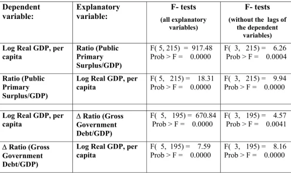
The F- tests presented in Table 2 allow us to reject the defined null hypotheses, accepting,

always at 1% level of significance, the causality between the growth of the real GDP per capita

and the public debt, which is measured by the ratios primary public surplus/GDP and gross

Government debt/GDP. Furthermore, it is clear that this causality is always bi-directional,

which is verified by the results of the two types of F-tests: one including all explanatory

variables (presented in the 3rd column of Table 2) and the other excluding the lags of the

dependent variables (presented in the last column of the same table).

3.4. Estimations without the lags of the dependent variables

To complement our analysis, we now use the more restricted model, estimating equations [3]

and [4] to test causality between the growth of the real GDP per capita and public debt, which,

as before, is represented by the ratio public primary surplus/ GDP, in levels, and the ratio gross

Government debt/ GDP, in first differences.

We continue to use F-tests to conclude about causality, but now we also consider the results of

the different R-squares in order to analyse the heterogeneity between the different OECD

countries included in our panel.

The results reported in Table 3 clearly confirm the bi-directional causality between GDP per

(12)

The R-squares presented in the last column of Table 3 are quite low, reflecting the

characteristics of the data (a panel constructed with data for 20 countries during a period of 14

years).

Therefore, on one hand, and according to the obtained values for the overall R-squared and the

R-squared “between”, we may conclude that there are differences in the behaviour of the

distinct countries, so that they should not be considered as a homogenous set. On the other

hand, looking at the values of the “within” R-squared, we confirm that the equations mainly

report the variations within each of the 20 countries during the considered period of 14 years.

3.5. Robustness analysis

In order to check the robustness of our results, we applied the same methodology using the

ratio net lending, Government/GDP as a measure of public debt. In addition, we tested the

methodology with the first differences of all the included variables. The obtained results are

not very different from those presented in this paper and are available from the author on

request.

4. Concluding remarks and policy implications

This paper empirically explores the Granger-causality relationship between economic

growth and public debt, adapting a methodology that was recently used by Erdil and

(13)

We confirm the existence of Granger causality between the growth of the real GDP per

capita and public debt, here represented by the ratio of the current primary surplus/GDP

and the ratio of the gross Government debt/GDP.

Furthermore, there is clear evidence that this causality is always bi-directional.

This result has important policy implications, since not only does public debt restrain

economic growth, but also real GDP per-capita growth influences the evolution of

public debt.

In addition, our findings point to heterogeneity across the considered OECD countries. These

countries not only face different initial conditions, but may also have heterogeneous relations

both between public debt and economic growth and between economic growth and public debt.

References

Diamond, P. (1965), “National Debt in a Neoclassical Growth Model”, American Economic Review, 55 (5), p. 1126-1150.

Erdil, E. and Yetkiner, I.H. (2008), “The Granger-causality between health care expenditure and output: a panel data approach”, Applied Economics, first published on 23 June 2008.

European Commission (2003), “Public finances in EMU – 2003” European Economy, No. 3/2003.

Holtz-Eakin, D., W. Newey and H. Rosen (1985), “Implementing Causality Tests with Panel Data, with an Example from Local Public Finance”, NBER Technical Working Papers, No. 0048.

Holtz-Eakin, D., W. Newey and H. Rosen (1988), “Estimating Vector Autoregressions with Panel Data”, Econometrica, 56 (6), p. 1371-1396.

Hurlin (2004), “Testing Granger causality in heterogeneous panel data models with fixed coefficients” mimeo, University of Orléans.

Hurlin and Vernet (2001), “Granger causality tests in panel data models with fixed coefficients” Working Paper Eurisco 2001-09, Université Paris IX Dauphine.

(14)

Levin, A, C. Lin and C. Chu (2002), “Unit Root Tests in Panel Data: Asymptotic and Finite Sample Properties”, Journal of Econometrics, No.108, p.1-24.

Mehrotra, A. N. and T. A. Peltonen (2005), Socio-Economic Development and Fiscal Policy – Lessons from the Cohesion Countries for the New Member States, ECB Working Paper Series, No. 467.

Modigliani, F. (1961), “Long-Run Implications of Alternative Fiscal Policies and the Burden of the National Debt”, Economic Journal, 71 (284), p. 730-755.

Nair-Reichert, U. and D. Weinhold (2001), “Causality tests for cross-country panels: a look at FDI and economic growth in less developed countries”, Oxford Bulletin of Economics and Statistics, 63 (2), p. 153-171.

Patillo, C., D. Romer and D. N. Weil (2002), External debt and growth, IMF Working Paper, No. 02/69.

Patillo, C., D. Romer and D. N. Weil (2004), What are the channels through which external debt affects growth?, IMF Working Paper, No. 04/15.

Perroti, R. (2002), Estimating the Effects of Fiscal Policy in OECD Countries, European Network of Economic Policy Research Institutes, Economics Working Papers, No. 015.

Presbitero, A. (2005), The Debt-Growth Nexus: A Dynamic Panel Data Estimation, Quaderno di Ricerca, No. 243, Dipartamento di Economia, Università Politecnica de Marche, Ancona, Italy.

Saint-Paul, G. (1992), “Fiscal policy in an Endogenous Growth Model”, Quartely Journal of Economics, No. 107, p. 1243-1259.

Schclarek, A. (2004), Debt and Economic Growth in Developing Industrial Countries, mimeo, available on-line in http://www.nek.lu.se/publications/workpap/Papers/WP05_34.pdf

Weinhold (1996), “Tests de causalité sur donnés de panel: une application à l’étude de la causalité entre l’investissement et la croissance”, Économie et prévision, 126, p. 163-175.

(15)

Appendix 1 - Descriptive statistics of the series*

Variable Mean Std. Dev. Min Max Observations

Log Real GDP, per capita

overall 2.150615 .8905783 .5022885 4.023911 N = 280 between .9109032 .5623209 3.88983 n = 20 within .0452437 1.992913 2.348052 T = 14

Ratio (Public Primary Surplus/GDP)

overall -.0292843 .0731284 -.9465867 .1179836 N = 280 between .0441778 -.1209672 .0717239 n = 20 within .059051 -.8549038 .0916828 T = 14

∆ Ratio (Gross Government Debt/GDP)

overall -.0055518 .0558991 -.656562 .1721613 N = 260 between .0169441 -.0576711 .0174049 n = 20 within .0533939 -.6274874 .1658475 T = 13

(16)

Table 1 – Panel-unit root tests – Levin-Lin-Chu

Variables lags coefficients t-value t-star P>t N

Log Real GDP, per capita 0 -0.33027 -9.038 -3.67602 0.0001 247 1 -0.49807 -14.246 -8.19794 0.0000 228 2 -0.77832 -17.474 -10.53592 0.0000 209

Ratio (Public Primary

Surplus/GDP) 0 -0.78199 -12.999 -7.69788 0.0000 247 1 -0.84965 - 11.462 - 5.02418 0.0000 228 2 -1.13491 -13.252 -5.87891 0.0000 209

∆ Ratio (Gross Government

(17)

Table 2 – Results for the model including the lags of the dependent variables*

Dependent variable:

Explanatory variable:

F- tests

(all explanatory variables)

F- tests

(without the lags of the dependent

variables)

Ratio (Public Primary

Surplus/GDP)

F( 5, 215) = 917.48 Prob > F = 0.0000

F( 3, 215) = 6.26 Prob > F = 0.0004

Surplus/GDP)

F( 5, 215) = 18.31 Prob > F = 0.0000

F( 3, 215) = 9.94 Prob > F = 0.0000

∆ Ratio (Gross

Government Debt/GDP)

F( 5, 195) = 670.84 Prob > F = 0.0000

F( 3, 195) = 4.57 Prob > F = 0.0041

F( 5, 195) = 7.59 Prob > F = 0.0000

F( 3, 195) = 8.16 Prob > F = 0.0000

(18)

Table 3 – Results for the model without the lags of the dependent variables*

Dependent variable:

Explanatory variable:

F- test R- Squares

Surplus/GDP)

F( 3, 217) = 6.78 Prob > F = 0.0002

within = 0.1561 between = 0.0148 overall = 0.0056

Surplus/GDP)

F( 3, 217) = 26.40 Prob > F = 0.0000

F( 3, 197) = 33.73 Prob > F = 0.0041

F( 3, 217) = 12.08 Prob > F = 0.0000