23 Journal of Applied Biomechanics, 2013, 29, 23-32
© 2013 Human Kinetics, Inc.
Alexandra Laurent and Annie Rouard are with the Sport Science Department, University of Savoie, Chambery, France. Vishvesh-war R. Mantha is with the Engineering Department, University of Trás-os-Montes-e-Alto Douro, Vila Real, Portugal, and with the Research Centre in Sports, Health and Human Development (CIDESD), Vila Real, Portugal. Daniel A. Marinho is with the Research Centre in Sports, Health and Human Development (CIDESD), Vila Real, Portugal, and with the Department of Sport Sciences, University of Beira Interior, Covilhã, Portugal. Antonio J. Silva is with the Engineering Department and with the Department of Sport Sciences, Exercise and Health, Uni-versity of Trás-os-Montes-e-Alto Douro, Vila Real, Portugal. Abel I. Rouboa (Corresponding Author) is with the Engineering Department, University of Trás-os-Montes-e-Alto Douro, Vila Real, Portugal; the Research Centre and Technologies of Agro-Environment and Biological Sciences (CITAB), Vila Real, Portu-gal; and the Department of Mechanical Engineering and Applied Mechanics, University of Pennsylvania, Philadelphia, PA.
The Computational Fluid Dynamics Study
of Orientation Effects of Oar Blade
Alexandra Laurent,1 Annie Rouard,1 Vishveshwar R. Mantha,2,3 Daniel A. Marinho,3,4
Antonio J. Silva,2 and Abel I. Rouboa2,5,6
1University of Savoie; 2University of Trás-os-Montes-e-Alto Douro; 3Research Centre in Sports,
Health and Human Development, Vila Real; 4University of Beira Interior; 5Research Centre and
Technologies of Agro-Environment and Biological Sciences, Vila Real; 6University of Pennsylvania
The distribution of pressure coefficient formed when the fluid contacts with the kayak oar blade is not been studied extensively. The CFD technique was employed to calculate pressure coefficient distribution on the front and rear faces of oar blade resulting from the numerical resolution equations of the flow around the oar blade in the steady flow conditions (4 m/s) for three angular orientations of the oar (45°, 90°, 135°) with main flow. A three-dimensional (3D) geometric model of oar blade was modeled and the kappa-epsilon turbulence model was applied to compute the flow around the oar. The main results reported that, under steady state flow conditions, the drag coefficient (Cd = 2.01 for 4 m/s) at 90° orientation has the similar evolution for the
different oar blade orientation to the direction of the flow. This is valid when the orientation of the blade is perpendicular to the direction of the flow. Results indicated that the angle of oar strongly influenced the Cd
with maximum values for 90° angle of the oar. Moreover, the distribution of the pressure is different for the internal and external edges depending upon oar angle. Finally, the difference of negative pressure coefficient Cp in the rear side and the positive Cp in the front side, contributes toward propulsive force. The results
indi-cate that CFD can be considered an interesting new approach for pressure coefficient calculation on kayak oar blade. The CFD approach could be a useful tool to evaluate the effects of different blade designs on the oar forces and consequently on the boat propulsion contributing toward the design improvement in future oar models. The dependence of variation of pressure coefficient on the angular position of oar with respect to flow direction gives valuable dynamic information, which can be used during training for kayak competition.
Keywords: kayak oar blade, computational fluid dynamics, pressure coefficient, propulsion
Kayak rowing is a competitive sport, and the kayak speed is related to three components: (i) the strength and the coordination of the kayaker which determine the force
transmission from the kayaker to the blade and to the boat (Aitken & Neal, 1992), (ii) the design of the boat which determines the drag (i.e., the force exerted by the water opposite to the boat displacement; Grare, 1985), (iii) the oar-blade system which transmits the force exerted by the kayaker (Mann & Kearney, 1980; Ackland, 2003). Different studies focused on the optimization of the race, concluding to the relationship between boat velocity and cycle parameters (frequency or length) related to kayak-er’s power (Dolnik & Krasnopievtsef, 1981). A few stud-ies were concerned with the kinematics of the blades for various paddling techniques (Plagenhoef, 1979; Issurin, 1980; Issurin et al., 1983; Kendal & Sanders, 1992). They concluded that the path of the blade must be parallel to the axis of the motion with a blade perpendicular to the boat during the propulsive phase. As the blade acts on the water, the blade did not remain fixed but presented slipping movement (Novakova, 1979; Plagenhoef, 1979; Mann & Kearney, 1980; Issurin, 1980; Issurin et al., 1983; Kendal & Sander, 1992; Di Puccio & Mattei, 2008). It was concluded that the flat blade allowed for increasing the boat velocity more quickly at the beginning of the race, whereas the curved blade would allow a gain of boat pace An Official Journal of ISB
www.JAB-Journal.com
during the race (Wargnier, 1990). Moreover, Kendal & Sander (1992) observed that the velocity with a curved blade is related to greater forward attack and to a blade path close to the boat axis. Few studies concerned the force exerted by the blade, which appeared determinant of the boat velocity (Issurin, 1980; Issurin et al., 1983). A few studies are published on the hydrodynamic of the blade although the kayak factories developed different designs with variation of shape, curvature and width.
Kayak paddle can be compared with a swimmer’s hand, which has been investigated from hydrodynamic approach (Marinho et al., 2010). The kayaker's force (or the swimmer’s force) is transmitted to the blade (or the swimmer’s hand), which propels the boat (or the body) through the water. The drag force is perpendicular to the direction of the movement of the hand or of the blade (Issurin, 1980; Issurin et al., 1983).
In swimming, based on kinematics or CFD, the drag force is strongly related to the orientation, the speed of the hand (Schleihauf, 1974; Berger et al., 1997; Rouboa et al. 2006), the size of limbs (Rushall et al., 1994; Berger et al., 1995; Gardano & Dabnichki, 2005; Marinho et al., 2008; Minetti et al., 2009), and the position of the fingers (Schleihauf, 1974; Takagi et al., 2001; Minetti et al., 2009; Marinho et al., 2010). Moreover, the drag coefficient is constant for all flow speed and all sweep back angles (Bixler & Riewald, 2002; Silva et al., 2005; Rouboa et al., 2006; Alves et al., 2007; Marinho et al., 2010). More recently, using 2D-CFD analysis, Gourgou-lis observed that the paddle increased the efficiency of the propulsion and the length of the stroke cycle (Gourgoulis et al., 2008).
In regard to (i) the new blade development, (ii) the lack of study on the hydrodynamic characteristics of the blades and (iii) the previous results obtained in swim-ming, the main goal of the current study is to evaluate the influence of the blade angle on the flow, in particular focusing on the local pressure coefficient using the CFD approach. We hypothesized that (i) the local pressure coefficient is not similar on all the surface of the paddle, with different values between the front and rear faces, (ii) the drag coefficient changes with the angle of the blade (45°, 90°, 135°), with a maximal value for the blade per-pendicular to the boat. These propositions are examined by 3D CFD approach as previous studies underlined the greater precision with 3D approach as compared with 2D approach (Rouboa et al., 2006; Zaidi et al., 2008). Results indicated that irrespective of the oar angle, the three Cp lines of the frontal side of the oar presented the similar shape but presented minor variation in Cp values along the reference line. Greater Cp was observed on the front face of the blade than on the rear one, irrespective the orientation of the blade was (45°, 90° and 135°). The pathlines colored with average flow velocity starting from frontal face of oar blade show recirculation zone at rear face of oar blade and average velocity around the kayak oar with rear side view, the pressure and pressure coefficient on the front side of kayak oar are presented. The pressure and pressure coefficient have maximum values in the central region and gradually fall toward the
both sides. The CFD approach could be a useful tool to evaluate the effects of different blade designs on the oar forces and consequently on the boat propulsion contribut-ing toward the design improvement in future oar models. The dependence of variation of pressure coefficient on the angular position of oar with respect to flow direction gives valuable information, which can be used during training for kayak competition.
Method
The closure problem of the turbulent modeling was arrived at, by using k-ε model with appropriate wall functions (Bixler & Riewald, 2002; Rouboa et al., 2006) using ANSYS FLUENT commercial CFD software. The k-ε model, is extensively applied and validated in the varied industrial applications (Raiesi et al., 2011). The k-ε model has been shown to be useful for free-shear layer flows with relatively small pressure gradients (Bardina et al., 1997). The present study is mainly focused on the variation of pressure coefficient due to angular orientation of oar blade with respect the flow direction excluding detailed flow characteristics (i.e., separation and reattachment of flow) including detailed turbulent effects. The system of equations for solving 3D, incompressible fluid flow in steady-state regimen is as follows: Continuity equation: ∂ ∂xi Ui
( )
= 0 (1) where i = 1, 2, 3.Navier–Stokes (momentum) equations: ∂ ∂xj rUiUj
(
)
= − ∂p ∂xi + ∂ ∂xj m+ mt(
)
∂x∂ j Ui( )
+ ∂ ∂xi Uj( )
⎛ ⎝⎜ ⎞ ⎠⎟− 2 3dijrk ⎡ ⎣ ⎢ ⎢ ⎤ ⎦ ⎥ ⎥ (2) where Ui( )t ≡ Ui+ ui is the component of instantaneous velocity in i-direction (m/s), Ui is the component of time averaged mean velocity in i-direction (m/s), ui is the com-ponent of fluctuating velocity in i-direction (m/s), i, j are the direction vectors, ρ is average fluid density (kg/m3), μis dynamic viscosity of fluid (kg/ms), μt is turbulent
vis-cosity of fluid (kg/ms), p is average pressure, k=1 2
( )
uiui the turbulent kinetic energy per unit mass (m2/s2); ε is adissipation rate of the turbulent kinetic energy per mass unit (m2/s3), d
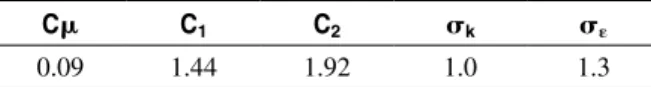
ij the Kronecker delta with the condition that, dij = 1 if i = j and dij = 0 if i ≠ j, the turbulent model constants σk, σε, C1, C2 are shown in Table 1.
Table 1 Modified k-𝛆 model constant
C𝛍 C1 C2 𝛔k 𝛔𝛆
0.09 1.44 1.92 1.0 1.3
Fluid Dynamics Study of Orientation Effects of Oar Blade 25
The equations of turbulence model: ∂k ∂xi rUi
( )
= ∂ ∂xj m+mt sk ⎛ ⎝⎜ ⎞ ⎠⎟ ∂k ∂xj ⎡ ⎣ ⎢ ⎢ ⎤ ⎦ ⎥ ⎥+ Pk− r´ (3) ∂´ ∂xi rUi( )
= ∂ ∂xj m+mt s´ ⎛ ⎝⎜ ⎞ ⎠⎟ ∂´ ∂xj ⎡ ⎣ ⎢ ⎢ ⎤ ⎦ ⎥ ⎥+ C1Pk ´ k− C2r ´2 k (4) The production of kinetic energy term is given as:Pk= −ruiuj ∂Uj
∂xi
= mtS2 (5)
where S the modulus of the mean rate-of-strain tensor is given by
S≡ 2SijSij (6) where the mean strain rate Sij is defined by
Sij= 1 2 ∂Ui ∂xj +∂Uj ∂xi ⎡ ⎣ ⎢ ⎢ ⎤ ⎦ ⎥ ⎥ (7)
The turbulent viscosity is calculated by the following relation:
mt = rCmk
2
´ (8)
To limit numerical dissipation, particularly when the geom-etry is complex inducing an unstructured grid, second-order discretization schemes are used (Figure 1). In generic terms, the convergence of the calculation is checked by the
value of the residuals of the various flow parameters. The convergence criteria in ANSYS FLUENT was set at 10–6.
This criterion is assumed sufficient to ensure the conver-gence of the solution for the current study. The boundary layer was created with aspect ratio algorithm with 4 rows of boundary layer grid cells with transition pattern of 1:1, with first row of grid at 0.01 mm immediately preceding wall grid with last percentage of 50% maintaining internal continuity. The first cell was 0.01 mm away from the blade producing mean y+ value was 1.09 and the tetrahedral grids
had maximum skewness of 0.74 and overall average skew-ness of 0.38. Appropriate number of tetrahedral grids cells in simulation model was arrived, which was an outcome of grid independence test carried out at the beginning of actual simulations. It was found that the difference in solu-tions for the drag coefficients for subsequent refinement in tetrahedral grid were less than 1%, when tested at an angle of 90° to flow direction.
Oar Blade Geometric Model
For this first study on CFD applied on oar motion in water, the most common blade was chosen (Macon model), which presented symmetrical form in relation to the oar axis (Figure 2).
The blade used in the numeric simulation was first modeled using a CAD commercial Software (Solidworks Inc, Concord, USA) to compute the 3D geometrical model (Figure 3). The oar blade front face surface area is 0.12758742 m2, length of blade is 0.72 m, width is 0.2 m.
Figure 1 — The computational mesh model showing boundary condition along with orientation of oar blade for individual case
under study.
26
Figure 3 — Computational geometrical model from SOLIDWORKS software.
Fluid Dynamics Study of Orientation Effects of Oar Blade 27
The 3D model is positioned in a rectangular geo-metrical domain and is meshed in GAMBIT (ANSYS FLUENT Inc, Sacramento, California) commercial meshing software. The boundary conditions were applied, the wall boundary condition of the oar surface, inlet and outlet surface at side surfaces and the symmetric bound-ary condition on the remaining exterior surfaces. Finally, the mesh model was exported to FLUENT software to simulate the flows around the oar.
The flow conditions were considered as following: • for this first approach of CFD in kayak, the flow was
considered as steady state with a horizontal velocity, U of 4 m/s, which corresponds to a Reynolds number (Re = UL/ν, with L denoting the blade’s length of 0.72 m and ν the fluid kinematic viscosity of water). As an initial condition, the water was assumed to be at rest.
• The pressure was set equal to zero for all the sides of the computational domain.
• The fluid was considered incompressible with den-sity of ρ = 996.6 kg·m–3 and dynamic viscosity of
water is 8.90 × 10⁻⁴ Pa·s at 25 °C.
• The action of the gravity force was set at g = 9.81 m·s–2 with the assumption of turbulence intensity of
1% at the inlet.
The oar was positioned stationery in the central part of the domain, the water flowed perpendicular to the oar. To simulate the different phases of the stroke, the flow was modeled for three different positions of the oar: 45°, which corresponded to the catch phase of the water; 90°, the major propulsive phase, which corresponds to the compressive phase (power phase); and 135°, which cor-responds to the end of the aquatic phase (Begon, 2006). The evaluation of the distribution of the local pressure on the oar was carried out along three imaginary lines along the length of oar blade, each on the front and rear sides of the oar blade. The location of these three lines were taken judiciously so as to reflect the average of pressure variation in nearby of three region i.e., internal, middle, external respectively (Figure 2) as per the location of the individual lines, which entailed the detailed analysis of pressure variation. This analysis can contribute in more specific geometric design modifications to decrease the drag by minimization of drag contributing regions of surface area respectively. The FLUENT simulation results allowed to get the Cp for each x-coordinate of each line
(internal, middle, external), for each side (front versus rear) and for each oar angle (45°, 90°, 135°). The study of variation of Cp along the respective lines was carried
out as Cp was most important component contributing
toward total drag coefficient and the propulsion obtained from the oar emerges to be essentially based on this drag component. The drag coefficient is obtained by the fol-lowing Equations (9):
CD= Fdrag
1
2r.V2.Aprojected
(9)
where Fdrag is drag force (about 2143 N), CD is drag
coefficient, ρ the average fluid density, V is average fluid velocity, Aprojected is the average projected cross-section
area (about 0.1333508 m2) in the flow direction, all in S.I.
units. The t test was applied to test for the difference in means for the different lines, the different sides, and the different angles (p < .05) (Ockerman & Goldsman,1999).
Results
Results indicated that irrespective of the oar angle, the three lines of the front side of the oar presented the similar shape of Cp curve along the x-axis (Figure 4).
For the three different orientations (45°, 90°, and 135°) the Cp curve could be divided into three parts. The first
part between 0 and 0.3x, which corresponded to the upper part of the blade (between the end of the handle and the beginning of the blade). For this first part, Cp is
different for the three different lines with a decrease for the middle line, an increase and then a decrease for the external and internal lines of drag coefficient. A constant drag coefficient characterized the second portion of the curve between 0.3 at 0.5x for the three lines (the middle part of the blade). The third part of the curve located between 0.5–0.8x (the end of the blade) presented similar Cp for the three lines with an increase from 0.5 to 0.7x
and decreases from 0.7 to 0.8x. Thus for all lines and all angles (45°, 90°, 135°), superior and unsteady Cp
values were observed at the extremities of the blade, with stable lower Cp for the central part of the blade. These
results clearly indicated a non-uniformity of Cp on the
front face of the paddle especially at the extremities of the oar.
Although there is similarity of the Cp curves
observed for the three oar angles, different values were observed for different angles of orientation with the main flow. The comparison of the stable portion showed greater Cp for an oar angle of 90° compared with 45° and
135° angles. To evaluate these differences, we compared the Cp of the three lines during the steady portion of the
curve (0.3–0.5x) for the front side. Results of the t test indicated significant differences between the Cp at 45°
and 90° (p = .00532), 90° and 135° (p = .0012) and not between 45° and 135° (p = .875). In other words, the oar force is greater, when the oar is perpendicular to the boat with no significant differences among the three lines indicating an homogeneous distribution of Cp values, on
the blade (Figure 5b). For the 45° blade angle, the Cp
was higher for the external line of the blade than for the middle and interior ones (Figure 5a). Opposite results were observed for the 135° blade angle with higher Cp
for the interior line than for the middle and exterior lines (Figure 5c).
The front side, presented minor variation of Cp values
whatever the orientation of the oar, and whatever the line of the oar (Figure 6). Cp is present on the entire front side
of the blade when the pressure appeared to vary only on few areas of the rear side with differences from one line to another. We can also observe that for both sides, the
Figure 4 — Pressure coefficients (Cp) on the x-coordinates
for the three angles (45°, 90°, 135°) for the three lines (interior, middle, exterior) of the front side.
pressure on areas appeared to vary similar whatever the orientation of the blade.
Greater Cp was observed on the front face of the
blade than on the rear one (Figure 7), whatever the ori-entation of the blade was (45°, 90° and 135°).
The pathlines plot colored with average flow velocity starting from frontal face of oar blade showing recircula-tion zone at rear face of oar blade and contour plots of average velocity around the kayak oar with rear side view, the pressure and pressure coefficient on the front side of kayak oar are presented in the Figure 8. The pressure and pressure coefficient have maximum values in the central region and gradually fall toward the both sides.
Discussion
For the first CFD study on kayak, the main goal was to evaluate the influence of blade angle on the flow. We hypothesized that (i) the pressure and the local pressure coefficient were not uniform regarding the surface of the
Figure 5 — Evolution of Cp for three attack angles (45°, 90°,
135°) for the three lines of the front side (interior, middle, exterior) at 4 m/s.
Figure 6 — Presence of the Cp (gray) and Cp null (white) for
the three lines, for both sides (front versus rear) and for three orientations of the oar.
Fluid Dynamics Study of Orientation Effects of Oar Blade 29
blade (internal, middle and external portions) and the side of the blade (front and rear), and (ii) the local pressure coefficient changed with the orientation of the blade with a maximum at 90° orientation angle of the blade.
Results pointed out that even if the fluid flow exerts different pressures on the blade, similar patterns of the local pressure coefficient on the x-axis were observed for the three blade angles (45°, 90°, 135°) and for the three lines (internal, middle, external) of the blade with higher values at the extremities and lower stable values for the central portion for the front side. As observed for the fin fish (Lauder et al., 2007; Zhu et al., 2008), the pressure is not uniform on all the surface of the blade reflecting different flow motions. The greater Cp at the handle-blade
junction is like the greater Cp observed at the fin-body
junction of the fish (Zhu et al., 2008). At this junction, water could not circulate around the handle-blade system (or body-fin for the fish) and, consequently, the pressure increased. The greater Cp at the free extremity could be
due to the smaller rounded surface at the end of the blade. A gradual increase of the local pressure coefficient was observed (Zhang et al., 2006) from the fin base to the fin
tip similar to the observed Cp increase from the top to
the tip of the blade in present study. The stability and the lower Cp in the central portion of the blade could be due
to the greater area and the uniform design of this portion. Despite the same Cp patterns for the three lines and
the three angles, results showed higher values for the blade angle of 90° and lower ones for 45° and 135°. The fluid did not exert the same force at 45°, 90° and 135°. These results were similar to those observed in swim-ming, with higher Cp for an attack hand angle of 90°
either quantified from a kinematic approach (Schleihauf, 1974) or from CFD (Bixler & Riewald, 2002; Rouboa et al., 2006; Marinho et al., 2010). In addition, for 90 °Cp is
not significantly different for all the portions of the blade (internal, middle and external). For this angle, the blade is perpendicular to the fluid flow, so the fluid hits this zone uniformly. In this position, the fluid cannot go around the blade, and consequently no vortex and no lift force can be created. In this case, the only propulsive force is the drag force applied uniformly on all the surface of the blade.
The nonsignificant differences between Cp values for
45° and 135° indicated that the fluid globally exerted the
Figure 7 — Pressure coefficients (Cp) on the x-coordinates for the three lines (interior, middle, exterior) of the front and rear sides
at 90°.
30
Figure 8 — For velocity of 4 m/s and 90 degree angle of oar with respect to the flow direction the (a) pathlines colored with
aver-age velocity starting from frontal face of oar blade, (a) contours of averaver-age velocity around the kayak oar blade, (b) contours of average pressure on kayak oar blade, (c) contours of average pressure coefficient of the kayak oar blade. (The online PDF version of this article contains this figure in color.)
Fluid Dynamics Study of Orientation Effects of Oar Blade 31
same pressure at the beginning and at the end of the oar motion in the water. Despite the similarities of Cp values,
the distribution of the Cp is not the same for 45° and 135°,
with superior Cp for the external edge compared with the
internal one for 45°, and converse by for 135°. These dif-ferences between the internal and external edges could reflect differences in lift forces for these angles and/or differences in vortex productions. Similar results have been observed on the fish locomotion (Liao, 2007). For example, a counter-clockwise vortex is visible at the head when the fish-body presented an angle of 100° with the direction of the fluid. The vortex moved to the middle of the body when the fish was at 180°, i.e., in the same direction as the fluid flow. It was concluded (Zhang et al., 2006) that the pressure is quite small at the leading edge area to reach its maximum at the trailing edge area. Thus, the repartition of Cp values changed with the orientation
of the oar, as did the undulation of the fish.
Finally big differences in Cp values were observed
between the rear and front sides of the oar. For the three blade angles, negative Cp was observed for the rear side
and positive Cp for the front one. Moreover, the rear
side presented some areas without any noticeable drag contributions. Similar results were observed for the swim-mer, for which the boundary layer separation resulted in formation of a low-pressure region behind the body (Naemi et al., 2009) and also on the fish. It was noticed (Dubois et al., 1974) that the pressure was positive in front of the fish and became negative at the back portion. It was concluded (Hirata, 2001) that pressure is negative at the opposite side of the propulsive side when the fish is swimming. The negative pressure can be explained from the Bernoulli principle: the water accelerated to pass around the fish, resulting in a decrease of the pressure (Dubois et al., 1974). The pressure difference between the front and rear sides created a force oriented from the high to the low pressures areas, i.e., from the front to the rear sides contributing to propel the boat.
The present study represented the application of CFD approach of the flow around the oar in kayaking. Results indicated that the angle of the oar strongly influenced the Cp with maximum values for a 90° angle of the oar.
Moreover, the distribution of the pressures is different for the internal and external edges depending of the oar angle. Finally, the difference of negative Cp in the rear side and
the positive ones in the front side contributed to create a propulsive force. The CFD approach could be a useful tool to evaluate the effects of different blade designs on the oar forces and consequently on the boat propulsion contributing toward development of new oar design.
References
Ackland, T.R., Ong, K., Kerr, D.A., & Ridge, B. (2003). Morphological characteristics of Olympic sprint canoe and kayak paddlers. Journal of Science and Medicine in Sport, 6, 285–294. PubMed doi:10.1016/S1440-2440(03)80022-1
Aitken, D.A., & Neal, R.J. (1992). An On-Water Analysis System for Quantifying Stroke Force Characteristics
during Kayak Events. International Journal of Sport Biomechanics, 8, 165–173.
Alves, F., Marinho, D., Leal, L., Rouboa, A., & Silva, A. (2007). 3-D computational fluid dynamics of the hand and fore-arm in swimming. Medicine and Science in Sports and Exercise, 9, 339.
Bardina, J.E., Huang, P.G., & Coakley, T.J. (1997). Tur-bulence Modeling Validation, Testing, and Develop-ment. NASA Technical Report Memorandum, 110446. Retrieved from http://www.ewp.rpi.edu/hartford/~jon gel/~/19970017828_1997026179.pdf
Bégon, M. (2006). Analysis and three-dimensional simulation of cyclical movements in a specific kayak ergometer (Unpublished doctoral dissertation, in French). Univer-sity of Poitier, Graduate School of Science Engineering, France.
Berger, M.A.M., de Groot, G., & Hollander, A.P. (1995). Hydrodynamic drag and lift forces on human hand/arm models. Journal of Biomechanics, 28, 125–133. PubMed doi:10.1016/0021-9290(94)00053-7
Berger, M.A.M., de Groot, G., & Hollander, A.P. (1997). Influ-ence of hand shape on force generation during swimming. In B.O. Eriksson, & L. Gullstrand (Eds.), Proceedings of XII FINA World Congress on Sports Medicine. (pp. 389-396). Goteborg: Chalmers University Reproservice. ISBN 91-630-6228-3.
Bixler, B.S., & Riewald, S. (2002). Analysis of swimmer’s hand and arm in steady flow conditions using computational fluid dynamics. Journal of Biomechanics, 35, 713–717.
PubMeddoi:10.1016/S0021-9290(01)00246-9
Di Puccio, F., & Mattei, L. (2008). Kayak rowing: Kinematic simulation of different techniques. Journal of Biomechan-ics, 41, 425–433. doi:10.1016/S0021-9290(08)70424-X
Dolnik, A., & Krasnopievtsev, I. (1980). Les fréquences de pagayage en canoe-kayak-USSR-Trad. Grebnoj Sport, 589, 39–43 (In Russian).
Dubois, A.B., Cavagna, G.A., & Fox, R.S. (1974). Pressure distribution on the body surface of swimming fish. The Journal of Experimental Biology, 60, 581–591. PubMed
Gardano, P., & Dabnichki, P. (2005). On hydrodynamics of drag and lift of the human arm. Journal of Biomechanics, 39, 2767–2773. PubMeddoi:10.1016/j.jbiomech.2005.10.005
Gourgoulis, V., Aggeloussis, N., Vezos, N., Antoniou, P., & Mavromatis, G. (2008). Estimation of hand forces and propelling efficiency during front crawl swimming with hand paddles. Journal of Biomechanics, 41, 208–215.
PubMeddoi:10.1016/j.jbiomech.2007.06.032
Grare, A. (1985). Study and realization of a data processing system for a flatwater kayak. (Unpublished doctoral dis-sertation, in French). University of Science and Technol-ogy of Lille, France.
Hirata, K. (2001). Principles of the Swimming Fish Robot (Unpublished master thesis). National Maritime Research Institute, Japan. Introduction available at http://www.nmri. go.jp/eng/khirata/fish/general/principle/index_e.html Issurin, V.B. (1980). The mechanism of stroke. Theory and
Practice in Physical Culture, 6, 50–53.
Issurin, V.B., Kransnov, E.A., & Ramuzov, G.G. (1983). Com-parative effectiveness of different variants of the technique of paddling in canoe-kayak. Theory and Practice in Physi-cal Culture, 9, 147–152.
Kendal, S.J., & Sanders, R.H. (1992). The technique of elite flatwater kayak paddlers using the wing paddle. Interna-tional Journal of Sports Biomechanics, 8, 233–250. Lauder, G.V., Anderson, E.J., Tangorra, J., & Madden, P.G.A.
(2007). Fish biorobotics: Kinematics and hydrodynamics
of self propulsion. The Journal of Experimental Biology, 210, 2767–2780. PubMeddoi:10.1242/jeb.000265
Liao, J.C. (2007). A review of fish swimming mechanics and behaviour in altered flows. Philosophical Transactions of the Royal Society B. Biological Sciences, 362, 1973–1993.
PubMeddoi:10.1098/rstb.2007.2082
Mann, R.V., & Kearney, J.T. (1980). A biomechanical analysis of the Olympic-style flatwater kayak stroke. Medicine and Science in Sports and Exercise, 12, 183–188. PubMed doi:10.1249/00005768-198023000-00010
Marinho, D.A. (2008). The study of swimming propulsion using computational fluid dynamics. A three dimensional analysis of the swimmer’s hand and forearm (Unpublished doctoral dissertation). Universidade de Tràs-os-Montes E alto Douro, Vila Real, Portugal.
Marinho, D.A., Barbosa, T.M., Reis, V.M., Kjendlie, P.L., Alves, F.B., Vilas-Boas, J.P., . . . Rouboa, A.I. (2010). Swimming propulsion forces are enhanced by a small finger spread. Journal of Applied Biomechanics, 26, 87–92. PubMed
Minetti, A.E., Machtsiras, G., & Masters, J.C. (2009). The Optimum Finger Spacing In Human Swimming. Journal of Biomechanics, 42, 2188–2190. PubMeddoi:10.1016/j. jbiomech.2009.06.012
Naemi, R., Chockalingam, N., Dunning, D.N., & Chevalier, T.L. (2009). A new method of measuring the Hydrody-namic Glide Efficiency in Swimming. A review. Journal of Science and Medicine in Sport, 13, 444–448. PubMed doi:10.1016/j.jsams.2009.04.009
Novakova, H., & Sukopp, J. (1979). Kinematic analysis of the art of canoe paddling speed. Theory of Physical Education, 27, 234–238 (In Czech).
Ockerman, D.H., & Goldsman, D. (1999). Student t-tests and compound tests to detect transients in simulated time series. European Journal of Operational Research, 116, 681–691. doi:10.1016/S0377-2217(98)00233-1
Plagenhoef, S. (1979). Biomechanical Analysis Of Olympic Flatwater Kayaking and Canoeing. Research Quarterly, 50, 443–459. PubMed
Raiesi, H., Piomelli, U., & Pollard, A. (2011). Evaluation of Turbulence Models Using Direct Numerical and
Large-Eddy Simulation Data. Journal of Fluids Engineering, 133, 193–203. doi:10.1115/1.4003425
Rouboa, A., Silva, A., Leal, L., Rocha, J., & Alves, F. (2006). The effect of swimmer’s hand/forearm acceleration on propulsive forces generation using Computational Fluid Dynamics. Journal of Biomechanics, 39, 1239–1248.
PubMeddoi:10.1016/j.jbiomech.2005.03.012
Rushall, B.S., Sprigings, E.J., Holt, L.E., & Cappaert, J.M. (1994). A re-evaluation of forces in swimming. Journal of Swimming Research, 10, 6–30.
Schleihauf, R.E. (1974). A biomechanical analysis of freestyle. Swimming Technique, 11, 89–96.
Silva, A., Rouboa, A., Leal, L., Rocha, J., Alves, F., Moreira, A., . . . Vilas-Boas, J.P. (2005). Measurement of swim-mer’s hand/forearm propulsive forces generation using computational fluid dynamics. Portuguese Journal of Sport Sciences, 5, 288–297.
Takagi, H., Shimizu, Y., Kurahima, A., & Sanders, R.H. (2001). Effect of thumb abduction and adduction on hydrodynamic characteristics of a model of the human hand. In J. Black-well and R.H. Sanders (Eds.) Proceedings of Swim Ses-sions XIX International Symposium on Biomechanics in Sports (pp. 122–126). San Francisco, California, June 26, 2001.
Wargnier, J.B. (1990). Studies in situ different Kayak Flatwater (Unpublished Master’s Project, in French). Free Institute Superior of EP, France.
Zaidi, H., Taiar, R., Fohano, S., & Polidori, G. (2008). Analysis of the effect of swimmer’s head position swimming per-formance using computational fluid dynamics. Journal of Biomechanics, 41, 1350–1358. PubMeddoi:10.1016/j. jbiomech.2008.02.005
Zhang, Y.H., He, J.H., Yang, J., & Zhang, A.W. (2006). A Computational Fluid Dynamics (CFD) Analysis of an Undulatory Mechanical Fin Driven by Shape Memory Alloy. International. Journal of Automation and Comput-ing, 4, 374–381. doi:10.1007/s11633-006-0374-4
Zhu, Q., & Shoele, K. (2008). Propulsion performance of a skeleton strengthened fin. The Journal of Experimental Biology, 211, 2087–2100. PubMed doi:10.1242/jeb. 016279