A computer vision approach to drone-based traffic analysis of road intersections

(1)

F

ACULDADE DE

E

NGENHARIA DA

U

NIVERSIDADE DO

P

ORTO

A computer vision approach to

drone-based traffic analysis of road

intersections

Gustavo Ramos Lira

Mestrado Integrado em Engenharia Informática e Computação Supervisor: Prof. Daniel Moura

Co-supervisor: Prof. Rosaldo Rossetti

(2)

(3)

A computer vision approach to drone-based traffic

analysis of road intersections

Gustavo Ramos Lira

Mestrado Integrado em Engenharia Informática e Computação

(4)

(5)

Abstract

In recent years, there has been interest in detailed monitoring of road traffic, particularly in in-tersections, in order to obtain a statistical model of the flow of vehicles through them. While conventional methods – sensors at each of the intersection’s entrances/exits – allow for counting, they are limited in the sense that it is impossible to track a vehicle from origin to destination. This data is invaluable to understand how the dynamic of a city’s mobility works, and how it can be improved. Therefore, new techniques must be developed which provide that kind of information. One of the possible approaches to this problem is to analyse video footage of said intersections by means of computer vision algorithms, in order to identify and track individual vehicles. One of the possible ways to obtain this footage is by flying a drone – a small unmanned air vehicle (UAV) – carrying a camera over an intersection.

Some work has been done with this solution in mind, but the usage of a top-down birds-eye perspective, obtained by flying the drone directly above the intersection, rather than at an angle, is limited or inexistent. This approach is interesting because it circumvents the problem of occlusions present in other footage capture set ups. The focus of this dissertation is, then, to develop and apply computer vision algorithms to footage obtained in this way in order to identify and track vehicles across intersections, so that a statistical model may be extracted. This model is based on said association of an origin and a destination. The algorithm employs background subtraction and vehicle tracking with Kalman filters. The most significant challenge was how to compensate for camera movement. Based on the implementation which was developed, this the approach proved useful for tracking cars, buses and trucks under some conditions.

(6)

(7)

Resumo

Recentemente, tem existido interesse na monitorização do tráfego automóvel, particularmente em cruzamentos, com o objectivo de obter um modelo estátistco do fluxo de veículos através dos ditos. Enquanto que os métodos convencionais - sensores em cada uma das entradas/saídas do cruzamento - permitem contar o número de veículos, estes são limitados, dado que não permitem acompanhar um veículo da entrada à saída. Estes dados são preciosos para perceber como funciona a dinâmica de mobilidade de uma cidade, e como pode ser melhorada, pelo que novas técnicas que forneçam esse tipo de informação têm que ser desenvolvidas. Uma das abordagens possíveis a este problema é a análise, por meio de algoritmos de visão por computador, de vídeo capturado dum cruzamento, para identificar e seguir veículos. Uma das formas possíveis de obtenção de vídeo é a utilização de um "drone" - um pequeno veículo aéreo não tripulado - com uma câmera, para voar por cima de um cruzamento e o filmar.

Algum trabalho foi feito com esta ideia em mente, mas a utilização de uma perspectiva vertical birds-eye, em vez de uma perspectiva inclinada, é limitada ou inexistente. Esta abordagem é inter-essante porque controna o problema das oclusões patente noutras formas de captura de imagem. O objectivo desta dissertação é, então, desenvolver e aplicar algoritmos de visão por computador a imagens obtidas desta maneira, para identificar e seguir veículos num cruzamento, para que um modelo estatístico do dito possa ser obtido. Este modelo baseia-se na supracitada associação de entradas a saídas. A solução desenvolvida passa pela utilização de background subtraction e de acompanhamento de veículos usando filtros de Kalman. Com base na implementação que foi de-senvolvida, esta abordagem parece ser útil para carros, autocarros e outros veículos semelhantes, sob determinadas condições.

(8)

(9)

Acknowledgements

I would like to thank my supervisors, Professor Daniel Moura and Professor Rosaldo Rossetti, for their work, dedication and invaluable advice, without which this dissertation would not exist.

I would also like to thank all of the faculty members who have motivated me and taught me over the past five years.

A word of appreciation to my friend Paulo Alcino for letting me bounce ideas off of him when I was stuck and for providing some spectacularly useful ideas himself.

I thank my parents, my friends and Sara for their support.

(10)

(11)

“Engineering stimulates the mind. Kids get bored easily. They have got to get out and get their hands dirty: make things, dismantle things, fix things. When the schools can offer that, you’ll have an engineer for life.”

(12)

(13)

List of Figures

2.1 An example of edge detection [McL10] . . . 7

2.2 An example of corner detection [figa] . . . 8

2.3 An example of blob detection [Guy08] . . . 9

2.4 An example of feature tracking [figb] . . . 10

2.5 Kalman filter being used to track a ball moving from left to right, even when occluded. The point where occlusion ends is marked in red [Kau] . . . 11

2.6 An example of background subtraction. In the lower half, white represents fore-ground and black represents backfore-ground [figc] . . . 12

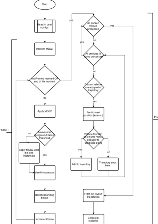
3.1 Flowchart of the general execution of the algorithm . . . 23

3.2 Distortion resulting from attempting to find a transformation matrix (left) and ref-erence frame (right) . . . 24

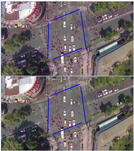
3.3 Same frame before (top) and after (bottom) blob filtering. Note the disappearance of the small blobs identified in the trees, zebra crossings and hanging wires. . . . 24

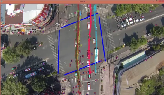
3.4 Example of the GUI being used to show each point in several trajectories . . . . 25

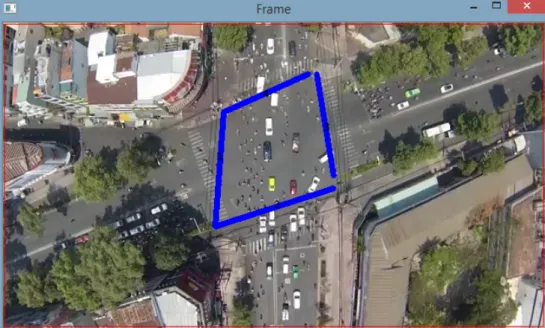
4.1 Identification of the source 1 intersection limits. 1 - left; 2 - bottom; 3 - top; 4 - right 29 4.2 Identification of the source 2 intersection limits. 1 - top left; 2 - bottom left; 3 - right 30 4.3 A group of motorcycles stopped in the middle of the intersection (highlighted in red) 37 4.4 Difference in level of zoom between clips 2 (top), 3 (middle) and 4/5 (bottom) . . 39

(16)

LIST OF FIGURES

(17)

List of Tables

4.1 Ground-truth values. Columns represents entrances and rows represent exits . . . 30

4.5 Distribution of traffic given the ground-truth values . . . 30

4.9 Ground-truth values. Columns represents entrances and rows represent exits . . . 31

4.12 Distribution of traffic given the ground-truth values . . . 31

4.15 Results for clip 1 in 360p . . . 32

4.27 Running times for clip 1 . . . 32

4.40 Running times for the clip 2 . . . 34

(18)

LIST OF TABLES

(19)

Abbreviations

CV Computer Vision MOG Mixture of Gaussians HDD Hard disk drive

(20)

(21)

Chapter 1

Introduction

This dissertation concerns itself with the development of a traffic analysis algorithm based on computer vision techniques, used on footage captured vertically above intersections using a drone. This field is of interest given the high value of gathering data about mobility and traffic patterns in an urban environment, which stems from the possibility of using this data to optimize urban traffic control systems such as traffic lights.

There is previous work regarding gathering data about traffic patterns, of which some has been done thanks to the video capture and subsequent analysis, but there no known implementation of a system where a drone is floated vertically over an intersection, and thus there is a gap in the field which can be worked on.

In the current chapter, the context, motivation and goals of the dissertation are presented, as well as an overview of the structure of the rest of the document.

1.1 Context

This work is positioned in the fields of computer vision and road traffic monitoring. These two fields intersect when one attempts to monitor road traffic by means of analysis of images captured by some video device positioned relative to the road.

Additionally, this research was done within the context of the Future Cities project, an Eu-ropean project that aims at improving the standard of living of cities’ populations by applying information technologies and for which Porto is a living lab.

This work was developed in the Faculty of Engineering of the University of Porto, within the Artificial Intelligence and Computer Science lab.

(22)

Introduction

1.2 Motivation

The motivation for this work is threefold: scientific, applicational and technological. Each of these is further detailed below.

The scientific motivation for this work is twofold: perform a gap analysis and experiment with computer vision techniques applied to road traffic monitoring. The first point equates to looking at the state of the art in these fields, seeing where there is work related to both, and then identifying where this work can be improved. For this purpose, a literature review of both computer vision techniques and road monitoring techniques and models has been done. The second point is related to the scientific interest of applying computer vision algorithms to the vertically captured images in order to identify why this situation might present challenges for those algorithms, and how these challenges could be conquered, if at all.

The applicational motivation is, of the three motivations identified, the one most rooted in real-world needs. The analysis of an intersection’s dynamic and the resulting data have incredi-ble potential: they allow for optimization of traffic signs’ timing, identification of possiincredi-ble bottle necks, prediction of traffic jams and modelling of a cities’ road-users behaviour, as well as the seeding of simulators [PRK11] which can then be used to predict and perfect the aforementioned tasks. This integration into simulators can be taken further, if one considers a whole platform ded-icated to transportation analysis [ROB07], a concept which is predicated on the idea of Artificial Transportation Systems [RLT11] [RE15].

The technological motivation is based around the idea of associating two previously indepen-dent technologies - drones and computer vision - to draw benefits from both and come up with a new system for traffic monitoring as an alternative to more traditional systems, such as road-level sensors.

1.3 Goals

The goal of this dissertation project is to design and implement an algorithm capable of identifying individual vehicles, based on computer vision techniques, and of tracking those vehicles through an intersection, to then build a statistical model of said intersection. Additionally, it is also a goal to test this algorithm with real-world footage to prove its reliability.

The project concerns itself with the development of an algorithm which extracts data from images captured from a top-down perspective. This perspective is interesting because it avoids the problem of occlusions, thus potentially facilitating the identification and tracking process. It has not been previously explored, but shows promise given the preliminary results here obtained.

The input images are assumed to be available already, and their means of capture is outside the scope of the research. Additionally, the camera is considered to remain in an almost fixed position above the intersection, with relatively low amounts of shaking. Traffic is assumed to flow unperturbed by jams or accidents and vehicles are considered to enter the intersection and one limit and exit at a different one, so u-turns shall be ignored.

(23)

Introduction

1.4 Document structure

Beyond this introduction, the current document is divided into another 4 chapters. In chapter2, several computer vision algorithms currently being used are described and analysed, and current road traffic monitoring algorithms are described, with their weaknesses and strong points identi-fied. Chapter3describes the solution which was developed, as well as the process which led to it. Chapter4shows the experimental results which were obtained. Finally, the conclusion can be found in chapter5. It provides an overview of what has been analysed, as well as a look into future work.

(24)

Introduction

(25)

Chapter 2

State of the art

This chapter presents an overview of current techniques in Computer Vision, and current research in traffic monitoring.

2.1 Computer Vision

Computer vision concerns itself with the analysis of visual data (both static and video) to extract information and convert it into some numeric form. It is closely related to the fields of AI, machine learning and mathematics. For this last one, specifically the areas of statistics and geometry.

It is commonly used to extract patterns or features from an image, with the intent of identifying objects which can then be counted or tracked, for various purposes. In the context of the current work, computer vision is interesting to analyse video footage of intersections in order to identify and track vehicles.

There are many computer vision techniques, depending on what kind of processing is to be done to the image. This chapter will focus on feature identification, feature tracking, background subtraction and morphological operations, because these four areas are the most prevalent when dealing with traffic monitoring.

There are also several different computer vision libraries which provide some of the algorithms mentioned further on. Some examples are OpenCV [Ope], VXL [Pro], IVT [IVT], AForge.NET [AFo] and the Mathlab Computer Vision System Toolbox [Mat]. When discussing different algorithms, it will be noted when these are implemented by OpenCV. This is because OpenCV is the library ex-pected to be used during the research phase, given that it is one of the most prevalent and complete ones.

2.1.1 Feature detection

Feature detection is any process by which points of interest (the features) are found on an image. They work by deciding for each pixel if it belongs to a feature or not. What a feature is varies depending on the goal of performing feature detection, because different applications consider different regions "interesting".

(26)

State of the art

Features are usually categorized in 4 different types: edges, corners, blobs and ridges. An edge is a boundary between two regions in an image, and is not necessarily a straight line. A corner is also known as an interest point, and corresponds to some isolated point in the image which differs from its neighbours in some way. Blobs are regions of interest similar to corners but composed of multiple points, rather than just one. Finally, ridges are considered to be sets of connected points where a certain function reaches a local maximum (similar to the geological concept of ridge - a series of elevations which forms an elongated crest). Similarly, a valley can be defined as a set of connected local minima. Further on, the focus will be on the first 3 types, as ridge detection has little to no application in vehicle tracking.

Feature detection is usually one of the first operations in a larger algorithm, so that some regions are isolated and then further analysed with other means. Because of this, it is critical that feature detection algorithms preform well and present good and accurate results. If the features are detected incorrectly, the whole algorithm will, most likely, preform badly.

2.1.1.1 Edge detection

Edge detection (figure 2.1) aims at finding boundaries which separate areas of a image with significantly different brightness. These are important because they usually correspond an object’s boundaries, a change in material or a change in lighting conditions in the source image. Ideally, one wants an edge detector to return a set of connected curves, but in practice this rarely happens because edges have discontinuities and are fragmented. However, this data is still useful and allows for significant reductions in processing time in further steps, because these no longer have to scan the whole image.

Edges are usually defined as sudden changes in brightness. Ziou and Tabbone go into detail regarding the different definitions of edges in [ZT88] but suffice it to say they are identified in one of two ways: either a local maximum in first-order derivative or a zero-crossing in the second-order derivative of the brightness function.

An edge detector can be evaluated according to three criteria defined by John Canny [Can86] 1. Good detection - minimize both false negatives and false positives, which corresponds to

maximizing signal-to-noise ratio;

2. Good localization - the points marked as belonging to an edge should be as close to the center of the edge as possible;

3. Single response - each edge should only be identified once.

In that same paper, Canny proposed his own algorithm for edge detection, which is to date still a very suitable algorithm. Nevertheless an extension was proposed by Deriche [Der87], and several other algorithms have been proposed. Most of these double as corner detectors and will be mentioned later, but one should be noted now: the Sobel operator, based around the notion of convolving the image to acquire an approximation of the derivative, is a filter designed to

(27)

State of the art

Figure 2.1: An example of edge detection [McL10]

emphasize edges in an image [RFW03]. Both the Canny algorithm and the Sobel operator are implemented in OpenCV.

2.1.1.2 Corner detection

Corner detection (see figure 2.2), also called interest point detection, is concerned with finding single, isolated points of interest in an image. These are useful for motion tracking/detection, for 3D modelling and for object recognition. Corners are defined as the intersection of two edges, however most so-called corner detectors actually detect points of interest in general, including isolated points with significant changes in color or brightness, for example.

Moravec defined one of the earliest algorithms designed to detect corners in [Mor80]. This algorithm had limitations pointed out by Moravec himself, and was further improved by Harris and Stephens [HS88]. Their algorithm can also be used to detect edges. It was further improved by Shi and Tomasi in 1994, who managed modify it so that it shows better results [ST94]. These later two algorithms are implemented in OpenCV.

2.1.1.3 Blob detection

Blob detection (see figure 2.3) focus on the identification of regions of interest in an image. A region of interest is defined as a set of connected points which share some common property such as brightness or color. This property can be constant, or vary within a range of values, but it will always be different from other points surrounding the blob.

Detection is usually either intensity-based or structure based. Intensity-based detection is based around the concept of defining the property being analysed as a function of position and then differentiating this function and looking for local maxima and minima, effectively looking for sudden changes in intensity in the picture. Structure-based detection relies on detecting features such as edges, curves and lines and then using this information to estimate where objects are located.

(28)

State of the art

Figure 2.2: An example of corner detection [figa]

Additionally, detectors can also be classified regarding their (in)dependence from scale: they can be fixed scale, scale invariant or affine invariant. These last ones are able of detecting features even when the image is subject to an affine transformation.

A common intensity-based method of blob detection is the Laplace of Gaussian (LoG). A Gaussian filter is first applied to the image. Afterwards, the Laplacian of this filtered image is taken, and blobs are considered to be located where the result takes extreme values (negative values for dark blobs and positive values for bright blobs). This process is analogous to using the Gradient to detect edges, but works for 2D structures [Voo87]. LoG suffers, however, from being sensitive to the size of the kernel used for Gaussian filtering and therefore not being scale invariant. Because of this, it is usually used in a scale-normalized fashion as defined by Lindberg [Lin98].

Lindberg also analysed another way of detecting blobs based around the concept of taking the determinant of the Hessian matrix of the Gaussian-filtered image. Once more, by locating maxima and minima, blobs are identified. [Lin12]

A significantly different approach to blob detection was proposed and used by Matas et al. in [MCUP02] to establish common points between two images taken from different perspectives. Their technique, named "Maximally stable extremal regions" is based around the concept of iden-tifying regions limited by a boundary which remain stable as long as possible when variating a brightness threshold which determines whether a pixel is within a region or not.

All of the aforementioned detectors are intensity-based. However, in 2007 Deng et al. pro-posed a structure-based detector named "Principal Curvature-Based Region Detector for Object Recognition" [DZM+07]. The idea behind PCBR is that while light intensity or color may change and therefore make intensity-based methods inadequate, there are structural elements of objects which can be used to identify them.

(29)

State of the art

Figure 2.3: An example of blob detection [Guy08]

2.1.2 Feature tracking

When dealing with sequences of images (that is, video), it is common that once features have been identified, one wants to track them across multiple frames to detect/describe motion of objects or of the camera, as exemplified in figure 2.4.

A common technique to achieve this is to apply the Lucas-Kanade algorithm [LK81] to esti-mate optical flow - the perceived motion of an object. This algorithm relies on two basic assump-tions [odtb]:

1. A pixel’s intensity remains constant between two consecutive frames. 2. Neighbouring pixels move in a similar fashion.

In fact, the Lukas-Kande algorithm takes the 3x3 matrix of pixels centred on the feature being considered and uses that patch for tracking. This algorithm, however, is only applicable if the motion is small enough. If the motion is too fast, it’s common to apply it iteratively, starting with low-resolution versions of the image and moving onto higher-resolution improving the model obtained with the coarser images [Hoi]. Further improvements have been achieved by carefully choosing the features to track by applying the Shi-Tomasi feature detector which was mentioned earlier. This forms the basis for the Kanade-Lucas-Tomasi feature tracker (often called KLT).

The algorithms described in the previous paragraph apply to tracking a set of sparse features. However, if one wishes to compute the optical flow of a dense set of points (e.g. all of the pixels in a frame), there is another algorithm, described by Farneback [Far03].

(30)

State of the art

Both Lucas-Kanade and Farneback’s algorithms are provided by OpenCV.

A different approach to feature tracking is the usage of a Kalman filter [WB95] to estimate the position of some interesting object. This technique is robust against occlusions (see figure 2.5) and has been used for vehicle tracking with success [SSFD11].

Figure 2.4: An example of feature tracking [figb]

2.1.3 Background subtraction

Background subtraction (see figure 2.6) aims at removing background information from an image, assuming all interesting objects are located in the foreground. It is usually applied to video data, and is based around building a model of the background (often initialized from some sub-set of the frames) and then subtracting that model from the frame being processed. It is useful to exclude useless data, and reduce the complexity of further processing steps. As Piccardi put it,

“Background subtraction is a widely used approach for detecting moving objects from static cameras.”

[Pic04]

The most significant step in background subtraction is the modelling of the background, as the quality of the results directly correlates to this. It is desirable that the model adapts to changes in

(31)

State of the art

Figure 2.5: Kalman filter being used to track a ball moving from left to right, even when occluded. The point where occlusion ends is marked in red [Kau]

illumination, to new objects entering the scene and remaining there and to the background varying in geometry.

Due to the limited computational resources of the past, it was not always possible to guarantee all of these properties. Therefore, methods have evolved over time. The earliest proposed methods simply modelled a pixel’s values over time by fitting a Gaussian probability density function by means of keeping a running average of the pixel’s values [WADP97] [KWH+94]. Later on, it was proposed that it might be more interesting to instead use the median value of the pixel’s last n values [LV01] [CGPP03].

The problem with both of these approaches, however, is that they do not consider the situation where a pixel might actually be inhabited by different background objects alternately (e.g. when foliage covers a building and moves back and forth due to wind). To mitigate this issue, Stauffer and Grimson presented a new method, by modelling each pixel as a mixture of Gaussians, and de-ciding which Gaussians represent background colors. Therefore, pixels are considered foreground if their value does not fit into any of the Gaussians which is considered as modelling a background color for that pixel [SG99].

The original Mixture of Gaussians as proposed by Grimson and Stauffer has been improved and modified over the years. The one proposed in [KB01] improves upon the original’s learning speed and accuracy and introduces shadow differentiation. This algorithm is known as MOG in OpenCV. Another variation, proposed by Zivkovic in [Ziv04], introduces the notion of varying the number of components for the mixture of Gaussians between pixels and over time, and therefore makes the algorithm more adaptable to changing environments. This algorithm is implemented in OpenCV as MOG2 [odta].

(32)

State of the art

Figure 2.6: An example of background subtraction. In the lower half, white represents foreground and black represents background [figc]

A different approach is the one proposed by Godbehere et al. in [GMG12] which is based around inferring which pixels belong to the foreground based on an Histogram of previous pixel values. The algorithm described in the paper also preforms feature tracking, but some implemen-tations are limited to the Background Subtraction portion.

2.1.4 Morphological operations

Morphological operations are binary operations on an image which are related to the shape (mor-phology) of the different structures in the image. In the context of Computer Vision they are normally used to remove noise and make detected features more prominent [Eff00].

They consist in placing a structuring element over all possible positions in an image, and applying some binary operation to the covered pixels based on their values as compared to those in the structuring element. The structuring element can be square, but can also be diamond-shape, cross-shaped, circular, or a myriad of other formats when interesting [Del].

The basic operations are erosion and dilation. Erosion consist in setting all pixels under the area covered by the structuring element to 0 when at least one of them isn’t 1 - effectively removing a layer of outer pixels from all regions in the image. Dilation does the opposite, setting all pixels covered by the structuring element to 1 if at least one of them is 1, and thus adding a layer of pixels.

(33)

State of the art

Erosion and dilation can further be combined to from two other interesting operations: opening and closing. Opening is an erosion followed by a dilation and takes its name from the fact that the resulting image will have any thin connections between elements opened into gaps. Closing is the opposite - a dilation followed by an erosion - and derives its name from closing any internal gaps in elements while keeping the outer size the same.

2.1.5 Overview

There are several areas of Computer Vision, each with different goals. This section looked into those which are considered to be related with the task at hand. Regarding the typical flow of a CV algorithm, generally speaking, one should first apply some sort of information filtering (background subtraction or feature detection), and then process the resulting data to find interesting data about the images being analysed (feature tracking, statistical treatment, etc.).

2.2 Traffic monitoring

Aside from existing Computer Vision techniques, explored in the previous section, it is also im-portant to take a look at existing road traffic monitoring solutions, as well as the associated models. 2.2.1 Road traffic monitoring solutions

Historically, there have been two very distinct ways of detecting road traffic: physical sensors placed on/near the road which detect the presence of a vehicle such as loop sensors, microwave detectors and pressure tubes, and computer vision solutions which apply computer vision algo-rithms to images captured by a camera aimed at the road and detect and count vehicles [Set97].

As established by Setchell, physical sensors provide useful data but are costly and cumbersome to install and maintain, which partially explains the motivation and advent of computer vision based tracking methods. These, in turn, can be divided into two broad categories: those based on fixed cameras and those based on cameras installed in UAVs.

2.2.1.1 Fixed camera

Fixed camera solutions consist in one or more cameras installed in, for example, a light pole or a road sign, in such a way that they can observe a considerable portion of the road. They’re installed at an angle and usually between 5m and 10m high. They may be able of panning, tilting and zooming, but it is not required.

It is worth nothing that the systems being discussed here are based on electronic cameras. There is previous work done with analogue equipment, such as that dome by Greenshields in the 1930s [Kü08] but given that the focus of this current work is to apply computer vision algorithms, this will not be considered.

These systems were first explored in [TSK+82] and then further reviewed by Iñigo in [Ini85] and [Ini89]. In his first paper, Iñigo noted that, at the time, there were no computer vision based

(34)

State of the art

road traffic monitoring systems in place except in Japan, largely because of the lack of compu-tational power and the high cost of cameras at the time. He predicted, however, that these costs would drop and make these solutions feasible. These predictions were reiterated in his second paper, where a CV based system is described, which detected vehicles by detecting changes in illumination along a line perpendicular to a lane being monitored. That same paper also mentions one of the major disadvantages of fixed camera systems: the obligatory presence of occlusions, because the camera is installed at an angle relative to the road. Additionally these systems also suffer from being relatively inflexible in the sense that they can not be easily moved and therefore only observe one specific stretch of road.

Later on, Koller et al. tackled the problem of Occlusion in [KWM94] by introducing a “Occlusion Reasoning” step into the vehicle tracking algorithm. Coifman et al., on the other hand, decided to track features instead of whole vehicles in an attempt to mitigate the same issue [CBMM98]. Rad and Jamzad proposed a solution which tracks vehicles by establishing bounding boxes and predicting where they might be next based on the size of the bounding box and a fixed. They also mitigate occlusion by tracking the centres of the bounding boxes and pre-dicting occlusion when they come too close together [RJ05].

More recently, Hsieh et al. have proposed a novel system which detects lane divisions and then uses that data to more easily distinguish between vehicles. Additionally, their system is also able to distinguish between different types of vehicles [HYCH06]. Also recent is some work which is based upon the idea of taking video streams from the internet and using those as data sources [LRB09].

2.2.1.2 UAV installed camera

An UAV (unmanned air vehicle) is an aircraft which, rather than having a pilot on board, is either controlled remotely or operates autonomously. These types of vehicles have been commonly referred to as “drones”. Although UAVs are commonly associated with military operations, and even though they were first developed with that purpose in mind [Sha], nowadays there are several civil and scientific applications for this kind of vehicle. One such is traffic monitoring, as surveyed by Kanistras et al. in [KMRV13]. Even though some of the solutions mentioned do not rely on video data, only those which do will be considered, given that the others are out of the scope of the current work.

When it comes to acquiring and analysing video data with an UAV, two major dimensions can be considered: whether the UAV moves or not while capturing data, and whether this data is analysed by an on-board computer, or transmitted to be analysed remotely.

The question of movement is important because if the UAV moves, the background will cer-tainly change drastically as the capturing of data goes on, and therefore background subtraction techniques are most likely not appropriate. In these cases, one will have to resort to tracking interesting features, and keeping track of the camera’s position relative to the road is almost a ne-cessity. An interesting algorithm which deals with detecting road features and limits is proposed

(35)

State of the art

in [Kim05]. On the other hand, if an UAV remains stationary over a section of road, background subtraction techniques similar to those used for stationary cameras might be of interest.

As far as data transmission goes, the question which must be asked is whether the available network provides enough throughput to transmit video data in real-time. Even if it does, there might be interest in having the actual UAV doing the processing itself, if one wishes it to react to changing traffic conditions (e.g. follow a traffic jam to locate the cause). If one opts to do the processing on the UAV itself, then the computational resources will most likely not be as plentiful as those available on the ground, so care must be taken to ensure the algorithm can run in real-time. 2.2.2 Models

Once data about how vehicles move is acquired, it is important to know how to use this data to model a section of road. There is some work regarding what these models should describe and how they can be generated.

2.2.2.1 Fundamental diagram of traffic flow

The fundamental diagram of traffic flow is a diagram first used by Greenshields [Kü08] to show the relationship between vehicle Speed, Flow and Density in a stretch of road. Flow is given as vehicles/hour, Density as vehicles/kilometre and Speed as kilometre/hour. Greenshields postulated that Flow = Density * Speed.

2.2.2.2 Statistical traffic models

As far as the generation of statistical models goes, the interesting variables are the aforementioned flow, density and speed, as well as, for intersections, mapping of entrances to exits in terms of numbers of vehicles. There as been some work regarding the generation of these models by Puri et al. [PVK07] and by Coifman et al. [CMM+06].

(36)

State of the art

(37)

Chapter 3

Solution

This chapter presents the algorithm which was designed to tackle to problem at hands, as well as the process which lead to the design choices which were made. Afterwards, the constraints that it imposes on the input data will be presented, as well as the implementation which was used for tests.

3.1 Overview

The general approach to the problem was that vehicles had to first be identified, to then be tracked. The result of the tracking process is a set of trajectories which are then used to build a model of the intersection.

The identification of vehicles is done with background subtraction. However, due to camera sway, sudden movements had to be detected and compensated against. Once that is done, blobs which are classified as foreground are considered vehicles and tracked from frame to frame.

The factors which led to choosing this approach, as well as the development process are de-tailed in section3.2.

3.2 Development process

This section describes the algorithm which was developed, along with the process which led to the choices which were made regarding which algorithms to use. The flowchart of the algorithm is shown in figure3.1.

The first step in developing the algorithm was to find a way to identify vehicles. The most common technique for this which was identified in previous research is background subtraction, so the choice was made to experiment with MOG, more specifically the MOG2 variant as imple-mented by OpenCV [Ziv04], due to its popularity and it being the most recent variation of MOG in that library. With the camera in a stable position this proved to work correctly. However, it was quickly discovered that camera instability led to MOG failing to correctly identifying foreground and background. In extreme cases, the whole frame would be considered foreground, as all of the

(38)

Solution

pixels had moved too far from their original position and none matched the statistical model kept by MOG. This led to the necessity of finding some stabilization technique.

The first attempt was to find some fixed features (such as rooftop details) in the image to be tracked from frame to frame, and to be used to infer a transformation matrix to be applied to the image, so that the image was distorted in order to bring objects back to their relative position before the camera shake. However, this proved unsuccessful, as there were no sufficiently unique features in the image to be tracked from frame to frame when the camera moved suddenly, and therefore the transformation matrix was wrongly inferred. This was observed empirically, by running the algorithm and looking at the transformed frames, which sometimes were grossly distorted, to the point where they were useless, as can be seen in figure3.2.

The second attempt was to calculate the optical flow of the image, to, again, infer a transfor-mation matrix. This too was unsuccessful, as the high amount of rapidly moving vehicles would introduce significant error into the calculation of optical flow.

The solution which, finally, was successful was to identify camera sway by monitoring the ratio of foreground pixels identified by MOG from frame to frame, and considering sway to be occurring when a sudden increase in this ratio was detected (via trial and error, a ratio threshold of 1.05 was found to work well). It should be noted that this increase depends on frame rate, and thus for different frame rates, the ideal value might be something other than the one which was identified. Once sway is identified, the algorithm then waits until the camera stabilizes (that is, the ratio drops below the threshold), and then interpolates between the last stable before instability occurred and the first stable frame following that section.

This choice proved to work well, but led to the choice of making the algorithm work in two phases, as it is first necessary to process the whole of the video to identify sections of instability, interpolate them and identify vehicles. Only once this is done, can the algorithm then move onto identifying the paths the vehicles take. This choice also facilitated the development process, given that it made it possible to first perfect the interpolation phase, and only afterwards move onto vehicle identification and path building.

As far as vehicle identification, the common technique in Computer Vision was used - once the foreground is identified, independent blobs are identified by finding their contours. Empirically, it was found that first running one erosion and two dilations on the frame improved results, as it removed noise and connected vehicles which might be split into two accidentally. This operation lead to, sometimes, two separate vehicles being identified as one single block. That problem is addressed further down.

Unfortunately, the result of the previous operation still proved to have a lot of false positives, so a filter had to be devised. Initially, the attempt was made to restrict the bounding box’s aspect ratio, but unfortunately this caused too many false negatives, as the bounding box would change ratio when vehicles turned, sometimes to values very close to those of the noise blobs’ bounding boxes. The choice was made to impose a restriction on the area of the blob’s bounding box. Because the area of the bounding box will change with the input resolution and the level of zoom

(39)

Solution

of the camera, this value had to be modifiable by the user, so it was included in the configuration file. The result of blob filtering is shown in figure3.3.

Once vehicles are identified, it is then necessary to track them from frame to frame. Because the sections of instability are interpolated, sometimes vehicles will appear to "freeze" and then jump forward. Additionally, sometimes vehicles will be partially occluded, for example, by cables hanging above the intersection. To mitigate these issues, a Kalman filter is used for each vehicle to predict its position in the following frame. This filter is initialized with the vehicle’s position when it first identified and the position of the vehicle closest to it (by Cartesian distance) in the next frame. Afterwards, the Kalman filter is used to predict the position of the vehicle in a following frame. If a vehicle is found sufficiently close to the prediction, it is considered the next vehicle. If it is not, then the prediction is used as the next position and the process continues. However, if no suitable match is found after 5 usages of the subsequent predictions, the trajectory is considered to have ended. This process prevents "losing" vehicles both due to interpolation of frames and due to a vehicle not being detected in a certain frame for whatever reason, but also, due to the limit of subsequent predictions, prevents the algorithm from artificially continuing a trajectory once the vehicle has effectively disappeared.

This process works when vehicles remain roughly on the same trajectory during periods of camera instability. Additionally, this process is also robust against vehicle merges due to proxim-ity, as it keeps a Kalman filter of each vehicle originally identified, and therefore when the vehicles separate each trajectory will be distinguished once again.

After all frames have been processed, only trajectories which intercept at least two limits are considered as being interesting. This eliminates cases where some noise at the edge of the frame or the middle of the intersection was considered to be a vehicle moving erratically. The limit they first intercept is considered the "entrance" they take, and the limit they intercept second is considered the "exit".

Finally, trajectories which differ from one another in less than 5% of their points are condensed into one trajectory. This is done because, sometimes, long vehicles are detected as multiple blobs, due to being partially occluded by cables or moving too fast, and are then tracked as multiple vehicles even if the blobs merge later on. This causes false positives which skew the count. The choice of 5% was based on the fact that these divisions occur, normally, at the entrance of the intersection, which accounts for roughly that amount in a vehicles trajectory.

The algorithm is strong against false positives thanks to the combination of ignoring blobs with nonsensical aspect ratios, as well as ignoring trajectories which do not both enter and exit the intersection or are clear duplicates of others. Ignoring trajectories which do not intersect an entrance, however, means that it does not consider any vehicles which were already inside the intersection when the video started. Therefore the algorithm requires a warm up period. On the other hand, this algorithm may ignore too much and therefore have an high ratio of false negatives, specifically in what concerns bicycles and motor bikes. This drawback could be minimized by improving the heuristic which filters the blobs to be tracked.

(40)

Solution

3.3 Technical details

3.3.1 Input data

The algorithm takes, as input, a video file to be analysed, a configuration file containing the list of lines which delimit the intersection and the expected minimum area in pixels of each vehicle, the number of frames to be skipped at the beginning of execution, the number of frames to be used for the learning phase of MOG, and, optionally, the maximum number of frames to process.

3.3.2 Output data

The algorithm returns, as output, a matrix of X by X (where X is the number of lines delimiting the intersection), containing the mapping of number of vehicles that enter the intersection at a certain limit, and exit at a certain limit.

3.3.3 Configuration file format

Because there are parameters which depend on the input video, such as the intersection’s limits, which are identified manually, it is necessary to feed this information into the algorithm. The choice was made to provide this information via a configuration file, so that these parameters can be stored permanently alongside the video, and to reduce the number of command line arguments. The configuration file is a plain-text file used to identify the limits of the intersection. It has a single number S on the first line, corresponding to the expected minimum area of a vehicle in pixels. It has a single number N on the second line, corresponding to the amount of intersection limits which will be listed, followed by N lines, specifying one limit each. A limit specification has four different numbers separated by spaces, corresponding to the starting x, starting y, ending x and ending y coordinates, respectively. These coordinates are specified in pixels.

3.3.4 Algorithm parameters

The solution uses several computer vision algorithms which take configuration parameters. These are detailed below.

3.3.4.1 MOG

MOG was configured with the following values:

• history: 1 - this value was chosen after preliminary testing suggested this worked well; • varThreshold: 16 - this is the suggested value on the openCV documentation pages; • bShadowDetection: false - there is no interest in detecting shadows;

• learning rate: 0.003 - once again, chosen due to preliminary testing suggesting this was a good value.

(41)

Solution

3.3.4.2 Kalman filter

The Kalman filters for each vehicle were all configured with the same values:

• Dynamic parameters: 4, corresponding to position and velocity in the x and y coordinates; • Measure parameters: 2, corresponding to position and velocity in the x and y coordinates; • Transition matrix:       1 0 1 0 0 1 0 1 0 0 1 0 0 0 0 1       Meaning that x_t+1= xt+ vxt yt+1= yt+ vyt vxt+1 = vxt vyt+1 = vyt

That is, it is assumed the velocity of vehicles traversing the intersection remains constant. • Process noise covariance matrix: 4 × 4 matrix with all values equal to 1 × 104 _-

empiri-cally found to be the lowest value which resulted in accurate predictions. Lower orders of magnitude would result in erratic predictions;

• Measurement noise covariance matrix: 4 × 4 matrix with all values equal to 0, given that measurements are assumed to be exact;

• Posteriori error estimate covariance matrix: 4 × 4 matrix with all values equal to 0. 3.3.4.3 Other parameters

Aside from the parameters of other algorithms which are used, the solution itself also has some parameters namely:

• Minimum area of blob bounding box: this parameter is alterable by the user, as it depends on the specific clip being analysed.

• Maximum distance between two subsequent positions of a vehicle: this value is used to prevent the algorithm from jumping between two unrelated vehicles. 30 pixels was origi-nally found to be a good value for the clip which was used for testing, and was kept as it worked well in all performed tests.

• Maximum number of subsequent predictions: Meaning the maximum amount of sub-sequent times the Kalman filter prediction can be used instead of an actual measurement.

(42)

Solution

5 was chosen because it was found that vehicles usually were not identified at most for 2 subsequent frames, and interpolations were usually, at most, 4 frames long.

3.4 Limitations

Due to the technique used to mitigate camera shake and the hard coding of the intersection limits, the camera must remain relatively static for duration of the video. Any permanent shift in perspec-tive leads to the algorithm not working. Any prolonged shake will cause too many frames to be missed and the tracking phase of the algorithm to not be able to follow the vehicles.

3.5 Implementation

The algorithm was implemented in C++, using the OpenCV library to represent and manipulate video images, as well as for its implementation of several computer vision algorithms which are used - MOG2, contour identification, minimum area rectangle identification and Kalman filters. The complete implementation can be found in

http://paginas.fe.up.pt/~ei10107/VehicleTrack.rar.

Additionally, the implementation has a GUI3.4which allows the user to navigate the results of the execution back and forward, inspecting identified vehicles and trajectories.

(43)

Solution

(44)

Solution

Figure 3.2: Distortion resulting from attempting to find a transformation matrix (left) and reference frame (right)

Figure 3.3: Same frame before (top) and after (bottom) blob filtering. Note the disappearance of the small blobs identified in the trees, zebra crossings and hanging wires.

(45)

Solution

(46)

Solution

(47)

Chapter 4

Experimental results

This chapter describes the process which was used to assess the solution described previously. The success metrics which are used will be considered first, followed by a description of the data set which was fed to the algorithm, and then the corresponding results and their analysis.

4.1 Metrics

One interesting metric for success is the percent of vehicles correctly identified and tracked - the amount of true positives. On the other hand, it is also important to measure the amount of false positives and false negatives as these can skew the statistical model. The analysis of false positives requires looking at the algorithm in action using the GUI which was developed, in order to check which of trajectories being identified don’t actually match a true vehicle.

The relationship between true positives (T P), false positives(FP) and false negatives(FN) is given by the following two formulas:

precision= T P T P+ FP recall= T P

T P+ FN

That is, precision measures how many items are accurate, of those identified, while recall measures how many items are identified, of those which should have been.

Another interesting metric is the distribution of traffic per pair of entrance/exit, based on per-centage of vehicles in that pair per total amount of vehicles counted. This distribution is rep-resented as a square matrix. Two of these distributions can be compared by using the matrix analogous of the Euclidean norm for vectors, given by the following formula:

d= p

tr((M − G)T_{× (M − G))}

nentrances

where M is the measured distribution, G is the ground-truth distribution and tr is the trace of the resulting matrix. This results in d being the square root of the sum of the squares of the differences

(48)

Experimental results

of each element of the matrices, divided by the number of entrances of the intersection. This division is necessary because different intersections have different numbers of entrances and it is desirable to normalize the value of d to compare between such cases.

The final metric is execution time - how fast the algorithm the input data is very important for real world applications. This depends both on the resolution of the input data and its complexity, as scenes with more camera shake or more vehicles are harder to process.

4.2 Setup and test cases

In order to test the algorithm, it would have been ideal to have access to multiple video clips with the desired characteristics (vertical perspective, high stability and considerable length). However, no clips within those parameters could be found beyond the one which was originally identified. To mitigate this issue, some footage was captured manually, emulating the perspective which would result from using an UAV.

Thus, there are two clip sources:

1. Source 1 A UAV-capture clip of a 4-way intersection in Vietnam which was extracted from an online source, and used to build the algorithm, as well as for testing

2. Source 2 A manually captured clip of a 3-way intersection in Porto, which was captured manually, and used exclusively for testing

Each source provided several clips all of which were processed in three different resolutions, all corresponding to a 16:9 aspect ratio:

• 720p - At 1280 by 720 pixels, commonly referred to as "HD"; • 480p - At 854 by 480 pixels;

• 360p - At 640 by 360 pixels;

In all cases, the algorithm was ran using the 250 frames preceding the clip to teach MOG2. All tests were preformed on the same machine - a PC running Microsoft Windows 8 64bit, with an Intel i7 4710HQ (2.50 GHz) processor, 12Gb of memory and reading the data from an HDD. 4.2.1 Source 1

Source 1 shows traffic flowing in a 4-way intersection, with 4 limits, identified in figure4.1. In this sub-section, traffic between 2 and 3 (and vice-versa) will be referred to as "vertical traffic" and traffic between 1 and 4 (and vice-versa) will be referred to as "horizontal traffic".

In order to have some diversity in the tests, this source was used in three different fashions: 1. Clip 1 - The entirety of the footage, which consists of essentially of 1.5 traffic light cycles.

That is, traffic flows vertically, then horizontally, and then vertically once again. The clip is 3 minutes and 10 seconds long, corresponding to 4750 frames;

(49)

Figure 4.1: Identification of the source 1 intersection limits. 1 - left; 2 - bottom; 3 - top; 4 - right

2. Clip 2 - 1000 frames, corresponding to the first 40 seconds, at the beginning of the clip, which consist of the first cycle of vertical traffic;

3. Clip 3 - 1000 frames, corresponding to the last 40 seconds, at the end of the clip, which consist of the second cycle of vertical traffic;

The period with the most horizontal traffic, roughly corresponding to the middle 2.5 minutes coincides with a period of high camera instability, and, at the very end, a very sharp zoom out, which means it is not as interesting to analyse as the other sections. This is why no partial clip was extracted from the middle of the original footage.

4.2.2 Source 2

Source 2 shows traffic flowing in a 3-way intersection which is highly irregular. Traffic flows uncontrolled by traffic lights, therefore vehicles cross paths often. Figure 4.2illustrates the en-trances/exits in this intersection. Two clips resulted from this source:

1. Clip 4 - 1 minute and 15 seconds of low density traffic, distributed nearly uniformly; 2. Clip 5 - 1 minute and 11 seconds of medium density traffic with most vehicles travelling

from entrance 1 to entrance 3

4.3 Characterization of the clips

Table4.1shows the number of trucks, cars and buses passing through the intersection from source 1 during the duration of each clip. Each table has 4 columns and 4 rows, representing each limit

(50)

Figure 4.2: Identification of the source 2 intersection limits. 1 - top left; 2 - bottom left; 3 - right

of the intersection. The number on cell (C,R) where C is the column number and R is the row number, represents the number of vehicles going from entrance C to exit R.

Table4.5shows the distribution of traffic based on the percentage of vehicles (out of the total for that clip) going from a certain entrance to a certain exit.

Table 4.1: Ground-truth values. Columns represents entrances and rows represent exits Table 4.2: Clip 1 1 2 3 4 1 0 0 5 10 2 3 0 23 0 3 0 25 0 0 4 21 4 0 0 Table 4.3: Clip 2 1 2 3 4 1 0 0 1 0 2 0 0 8 0 3 0 13 0 0 4 0 0 0 0 Table 4.4: Clip 3 1 2 3 4 1 0 0 3 0 2 0 0 8 0 3 0 5 0 0 4 0 1 0 0

Table 4.5: Distribution of traffic given the ground-truth values Table 4.6: Clip 1 1 2 3 4 1 5% 11% 2 3% 25% 3 27% 4 23% 4% Table 4.7: Clip 2 1 2 3 4 1 5% 2 36% 3 59% 4 Table 4.8: Clip 3 1 2 3 4 1 18% 2 47% 3 29% 4 6%

The number of motorcycles is not shown because, unfortunately, the detection rate on motor-cycles is close to null. There are a series of reasons for this which will be explored at the end of the current chapter.

(51)

Table4.9 shows the number of vehicles passing through the intersection during the duration of each clip from source 2. Each table has 3 columns and 3 rows, representing each limit of the intersection. The columns and rows have the same meaning as before

Table4.12shows the distribution of traffic based on the percentage of vehicles (out of the total for that clip) going from a certain entrance to a certain exit.

Table 4.9: Ground-truth values. Columns represents entrances and rows represent exits Table 4.10: Clip 4 1 2 3 4 1 0 3 2 2 0 0 1 3 3 2 0 Table 4.11: Clip 5 1 2 3 4 1 0 0 2 2 3 1 0 3 10 1 0

Table 4.12: Distribution of traffic given the ground-truth values Table 4.13: Clip 4 1 2 3 4 1 27% 18% 2 9% 3 27% 18% Table 4.14: Clip 5 1 2 3 4 1 12% 2 18% 6% 3 59% 6%

This data in all of the aforementioned tables is used as the ground-truth in further analysis.

4.4 Results

This section shows the counts obtained by the algorithm for the 5 clips in each of the 3 resolutions. It also shows the amount of true positives and false positives/negatives, as well as the precision and recall measurements.

Additionally, it presents the traffic distributions, and respective comparisons to their analogous in the ground-truth.

The experimental results for source 1 showed very poor detection rate for motorcycles (close to or actually 0%, depending on the clip and resolution). Therefore, the results which follow are mostly based on the detection of cars, trucks and buses. However, because some motorcycles were in fact detected, they need to be accounted for, otherwise the number of false positives would be artificially inflated.

On the other hand, for source 2 motorcycles did not prove to be a challenge, therefore they are not considered a special case and are simply counted normally.

4.4.1 Clip 1

(52)

Table 4.15: Results for clip 1 in 360p

Table 4.16: Vehicle count 1 2 3 4 1 0 1 0 4 2 2 0 4 0 3 1 7 0 3 4 5 1 0 0

Table 4.17: Vehicle distribution

1 2 3 4 1 4% 14% 2 7% 14% 3 4% 25% 11% 4 18% 4% Table 4.18: Measure-ments for clip 1 in 360p

True positives 23 False negatives 68 False positives 3 Motorcycles 2 Precision 88.5% Recall 25.3% d 0.0468 Table 4.19: Results for clip 1 in 480p

1 2 3 4 1 2% 2% 12% 2 2% 17% 5% 3 31% 5% 4 19% 5% Table 4.22: Measure-ments for clip 1 in 480p

True positives 37 False negatives 54 False positives 2 Motorcycles 3 Precision 94.9% Recall 40.7% d 0.0321 Table 4.23: Results for clip 1 in 720p

1 2 3 4 1 6% 3% 21% 2 13% 6% 3 4% 25% 6% 4 11% 3% 4% Table 4.26: Measure-ments for clip 1 in 720p

True positives 49 False negatives 42 False positives 12 Motorcycles 11 Precision 80.3% Recall 53.8% d 0.0591 Table 4.27: Running times for clip 1

Resolution Time (s)

360p 72

480p 122

720p 302

Overall, the accuracy increases with the resolution, but so does the processing time, as ex-pected. The low accuracy for all three resolutions will be explained further on.

(53)

4.4.2 Clip 2

The results for clip 2 are in tables4.28,4.32,4.36and4.40.

1 2 3 4 1 2 40% 3 60% 4 Table 4.31: Measure-ments for clip 2 in 360p

True positives 10 False negatives 12 False positives 0 Motorcycles 0 Precision 100% Recall 45.5% d 0.0148

Table 4.33: 1 Vehicle count 1 2 3 4 1 0 1 0 0 2 1 0 4 0 3 0 6 0 0 4 0 2 0 0

1 2 3 4 1 7% 2 7% 29% 3 43% 4 14% Table 4.35: Measure-ments for clip 2 in 480p

True positives 10 False negatives 12 False positives 2 Motorcycles 2 Precision 83.3% Recall 45.5% d 0.0638

1 2 3 4 1 13% 3% 3% 2 7% 23% 3 43% 4 3% 3% Table 4.39: Measure-ments for clip 2 in 720p

True positives 21 False negatives 1 False positives 5 Motorcycles 4 Precision 80.8% Recall 95.5% d 0.0650 The results for this shorter clip are, overall, better than those for the first clip, and particularly in the case of the 720p version, much better. Again, this will be explored in the analysis section. 4.4.3 Clip 3

(54)

Table 4.40: Running times for the clip 2 Resolution Time (s)

360p 20

480p 33

720p 75

1 2 3 4 1 2 3 100% 4 Table 4.44: Measure-ments for clip 3 in 360p

True positives 1 False negatives 16 False positives 0 Motorcycles 0 Precision 100% Recall 5.9% d 0.2171 Table 4.45: Results for clip 3 in 480p

1 2 3 4 1 2 33% 3 67% 4 Table 4.48: Measure-ments for clip 3 in 480p

True positives 3 False negatives 14 False positives 0 Motorcycles 0 Precision 100% Recall 17.6% d 0.1096 Table 4.49: Results for clip 3 in 720p

1 2 3 4 1 4% 12% 2 32% 4% 3 4% 28% 4% 4 4% 4% 4% Table 4.52: Measure-ments for clip 3 in 720p

True positives 15 False negatives 2 False positives 10 Motorcycles 0 Precision 60% Recall 88.2% d 0.0617

As with clip 2, this clip shows better results than the first one, and better results the higher the resolution. However, the improvement is not quite as noticeable.

(55)

Table 4.53: Running times for clip 3 Resolution Time (s)

360p 21

480p 29

720p 89

4.4.4 Clip 4

The results for clip 4 are in tables4.54,4.58,4.62and4.66.

Table 4.55: Vehicle count 1 2 3 1 0 0 2 2 0 0 0 3 2 0 0

1 2 3

1 50%

2 3 50%

Table 4.57: Measure-ments for clip 4 in 360p

True positives 4 False negatives 7 False positives 0 Precision 100% Recall 36.36% d 0.1728

1 2 3

1 14% 29%

2

3 43% 14%

1 2 3

1 13% 25%

2 13%

3 38% 13%

(56)

360p 32

480p 42

720p 140

4.4.5 Clip 5

The results for clip 5 are in tables4.67,4.71,4.75and4.79. Table 4.67: Results for clip 5 in 360p

1 2 3

1 33%

2

3 50% 17%

1 0 .

1 9%

2 9%

3 73% 9%

True positives 10 False negatives 7 False positives 1 Precision 90.91% Recall 58.82% d 0.0843

Table 4.77: Vehicle distribution 1 2 3 ]

1 17%

2 8% 8%

3 67%

True positives 10 False negatives 7 False positives 2 Precision 83.33% Recall 58.82% d 0.0294 36

(57)

360p 31

480p 42

720p 135

4.5 Analysis of results

First and foremost, it is noticeable that motorcycles tracking success rate is very poor in source 1, as there are several dozens motorcycles traversing the intersection. The author suspects this is due to two main reasons:

1. The fact that motorcycles are physically smaller, and therefore harder to detect. This is supported by the fact that during clip 2 some motorcycles are tracked, while during clip 3 none are, and clip 3 is taken with a lower level of zoom, therefore making the vehicles physically smaller on screen (see figure4.4). The fact that the motorcycle detection rate is also lower on lower resolutions also supports this theory, as well as the fact that motorcycles are tracked correctly in the footage from source 2, in which they occupy a much more significant area on the screen;

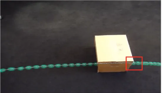
2. The chaotic movement of motorcycles trough the intersection, sometimes even completely stopping in packs in the middle of the road, makes it difficult for the algorithm to track them from frame to frame (see figure4.3).

Figure 4.3: A group of motorcycles stopped in the middle of the intersection (highlighted in red)

On the other hand, the car/truck/bus recall, especially for clips 2 and 3 in high resolutions, is interesting, being above 85% and coupled with precisions sometimes above 80%. Also interesting

A computer vision approach to drone-based traffic analysis of road intersections

F

E

U

P

A computer vision approach to

drone-based traffic analysis of road

intersections

Gustavo Ramos Lira

A computer vision approach to drone-based traffic

analysis of road intersections

Gustavo Ramos Lira

Mestrado Integrado em Engenharia Informática e Computação

Abstract

Resumo

Acknowledgements

Contents

List of Figures

List of Tables

Abbreviations

Chapter 1

Introduction

1.1

Context

1.2

Motivation

1.3

Goals

1.4

Document structure

Chapter 2

State of the art

2.1

Computer Vision

2.2

Traffic monitoring

Chapter 3

Solution

3.1

Overview

3.2

Development process

3.3

Technical details

3.4

Limitations

3.5

Implementation

Chapter 4

Experimental results

4.1

Metrics

4.2

Setup and test cases

4.3

Characterization of the clips

4.4

Results

4.5

Analysis of results