STOXX EUROPE 600 Index – CORPORATE DEBT
MATURITY ANALYSIS
Jorge Augusto Barreiros Magalhães
Master in Finance
Thesis supervisor:
Prof. Doutor Luís Miguel da Silva Laureano, ISCTE Business School, Assistant Professor, Department of Finance
i
Abstract
This dissertation consists of an empirical study about corporate debt maturity structure in STOXX EUROPE 600’ firms. The observation period dates from year 2000 to 2013. Balance sheet yearly observations were used to build firm specific variables (determinants) to use in the model. Through different techniques of regression analysis we assess the changes in the relevance of the determinants in explaining debt maturity by model and throughout the sample period with particular focus to the periods before and after the 2008 subprime crisis. A complementary study on Euro Area yield curve AAA volatility also provides plausible evidence to support main conclusions. The results suggest an optimized structure trend of debt into firm’s balance sheet. A flat amount of debt remains since 2008 but, short-term debt has been replaced by long-term debt, thereby causing an increase of the debt maturity ratio. The specific purpose analysis to Euro Area Yield curve AAA revealed that shorter time interest rates had their volatility in highest levels after the subprime crisis, making riskier for firms to finance themselves using short-term strategies, suggesting this fact to be one plausible cause for the preference for long-term debt. Liquidity determinant dramatically lost his significance after the subprime crisis, while Growth Options determinant increased his. The results also suggested that debt maturity decision is not driven only by firm specific factors, i.e. macro-economic factors also contribute to impact debt maturity, but in a more significant way after the 2008 subprime crisis than before.
Key words: Debt maturity, capital structure, determinants, subprime.
ii
Resumo
Esta dissertação consiste num estudo empírico sobre a estrutura da maturidade da dívida das empresas do índice STOXX EUROPE 600. O período de observação utilizado é 2000 a 2013. Foram utilizados dados contabilísticos de frequência anual para construção dos determinantes a usar no modelo. Usando diferentes técnicas de regressão avaliamos a alteração de importância dos determinantes em termos de capacidade de explicar o comportamento da maturidade da dívida com especial foco para os períodos que antecedem e precedem a crise do subprime. Os resultados sugerem uma tendência para a otimização da estrutura da dívida por parte das empresas. O montante de dívida nos balanços das empresas permanece constante desde 2008 assistindo-se simultaneamente a uma substituição da dívida de curto prazo por dívida de longo prazo resultando num aumento do rácio de maturidade da dívida. A análise complementar da volatilidade da yield curve na Zona Euro de rating AAA revelou que as taxas de juro para períodos de curto prazo registaram grande volatilidade depois do subprime, tornando assim mais arriscado para as empresas usarem estratégias de financiamento de curto prazo e por sua vez tornando preferível o financiamento de longo prazo. O determinante Liquidity perdeu dramaticamente a sua importância depois do subprime e o determinante Growth Options aumentou significativamente o seu impacto. Os resultados sugerem também que outros fatores para além dos específicos, ou seja, fatores macroeconómicos, também contribuem para explicar a maturidade da dívida e de forma mais relevante depois do subprime.
Palavras-Chave: Maturidade da Dívida, estrutura de capital, determinantes, subprime.
iii
Acknowledgements
I would like to thank to my supervisor, Professor Luís Miguel da Silva Laureano for the helpful comments, suggestions and availability demonstrated during this journey.
I would also like to thank to my family for the unconditional support and motivation. To all my friends and colleagues a word of appreciation for the time we spend together.
My special acknowledgement goes to my grandmother for her daily caring and important support given to me.
iv Contents Abstract i Resumo ii Acknowledgements iii Contents iv List of Tables v List of Figures vi 1. Introduction 1 2. Review of Literature 3 2.1. Agency Costs 4
2.2. Taxes Based Model 5
2.3. Liquidity Risk (Credit Risk) 6
2.4. Asymmetric Information and Signaling 7
2.5. Debt/Asset maturity matching 7
2.6. Reference to empirical studies 8
3. Sample and Data Description 11
3.1. STOXX Europe 600 Index 11
3.2. Firm-Specific Variables 12
4. Methodology 15
5. Empirical Results and Discussion 19
5.1. Descriptive Statistics Analysis 19
5.2. Correlation Analysis 22
5.3. Regression Analysis 22
5.3.1. Analysis of Determinants 23
5.4. Final Remarks about subprime impact on debt maturity decision 26 6. Conclusion, limitations and further research 31
Bibliographic References 33
Appendix 1 35
v
List of Tables
Table 1: Overview of data obtained from Bloomberg: number of observation by year and
variable 35
Table 2: Overview of the firm-specific variables presenting the number of observations by
each year and variable 37
Table 3: Descriptive Statistics of firm specific variables for whole period (2000-2013) 28
Table 4: Descriptive Statistics of firm specific variables for sub-period (2000-2007) 28
Table 5: Descriptive Statistics of firm specific variables for sub-period (2008-2013 28
Table 6: Descriptive Statistics of Debt Maturity by year 28
Table 7: Debt maturity average ratios for each year across industry sectors 29
Table 8: Correlation matrix 22
Table 9: Regression coefficients and its statistical significance for all models 23
vi
List of Figures
Figure 1: Distribution of the number of observations for each year 36
Figure 2: Distribution of the number of observations for each variable 36
Figure 3: Disparity of each year to the target value of observations per variable 38
Figure 4: Total number of observations by each variable to include in the model 38
Figure 5: Debt maturity trend for whole sample 20
Figure 6: Decomposition of Total Debt evolution by short and long-term debt across whole
sample 21
Figure 7: Debt Maturity Levels for whole sample by Industry Sectors 30
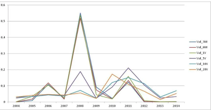
Figure 8: Interest rate daily volatility from 2004 to mid 2014 (rated AAA Euro Zone Yield
1
1. Introduction
This dissertation is focused into firms’ capital structure scope, more specifically debt maturity issues. The topic intends to address how a firm chooses its optimal debt maturity structure or, in other words, what are the main factors that can drive the firm’s debt maturity structure decision.
Capital structure theme has been strongly debated and studied by many academics in the past years since the famous Modigliani and Miller (58, 63). There are many thesis and working papers addressing this theme through time, showing us the relevance and the complexity of the topic to the business world. And, as it is known, the last years since the 2008 crisis have been particularly challenging for the firms to run their business with more constrains regarding financing, more directly debt-financing, (but also equity financing too, because shareholders’ investments many times are financed with loans) as the banking sector got strongly penalized with the subprime crisis.
The subprime affected financial markets and its confidence. Financing became much more difficult and expensive. Financial crisis spread out for all over the world affecting individual countries financial systems where the banks suffered with their exposures. Banks play an important role for the economies and their situation quickly impacted other industries and even more quickly those effects reached societies. Here is when central banks get into the scene. Recently implemented economy “boosting” measures to help several economies recovering, as decreasing interest rates, Quantitative Easing programs, other assets purchase programs, sovereign loans, aiming countries finance themselves more easy and cheaper, avoiding bailouts and fomenting financial institutions to lend money to boost industries and consumption and overall economy. Low inflation (CPI) scenarios are now concerning central banks, new low records in interest rates are observable, and financing has become cheaper. Government and corporate Bond yields are at low levels while S&P 500 is constantly reaching record highs while signs of real economy recovery prevail weak.
The intention of this work is to explore and show what specifically changed in firm’s debt maturity structure in times where the access to financing became much more difficult and the overall credit market is more constrained by comparing periods before and after the subprime crisis and trying to provide empirical evidence of plausible facts that might explain those changes. Also by observing the changes in the relevance of determinants to properly access its
2 importance in Debt Maturity trend before and after de subprime crisis. The empirical study uses as base financial information from STOXX EUROPE 600 index and respective data samples from 2000 to 2013. Two sub-periods will be considered to infer about the impact of subprime on debt maturity structure, 2000-2007 and 2008-2013.
The methodology used in this work is the econometric regression model to estimate the coefficients for the determinants of debt maturity. Fixed-effects regression and random-effects regression were used to better capture both individual effects, time effects and unobserved effects that impact debt maturity as we are working with panel data. We also perform descriptive statistics and correlation analysis.
A specific purpose analysis to Euro Area Yield Curve AAA (spot prices) was performed to support the argument of the decrease of importance of Liquidity determinant after subprime crisis and also to support the observable preference for long-term debt rather than short-term debt also after the subprime. This analysis consists in a yield volatility trend from year 2004 to mid 2014.
Our main results suggest that debt maturity ratio has been increasing since the beginning of our data sample period (year 2000) and it slowed down the pace in 2008 by stabilizing until the end of year 2013. This behavior resulted of a change in the debt maturity structure where firms started to prefer to finance themselves with long-term debt rather than short-term keeping flat the amount of debt in their balance sheets. Our results also suggest that the Liquidity determinant become irrelevant to explain debt maturity after the subprime crisis, whereas the Growth Options determinant increased its power to explain debt maturity. The analysis on Euro Area Yield Curve AAA show that short-term interest rates had their highest levels of volatility in years 2008 and 2011 when the markets were more stressed. We associate this fact with both liquidity determinant loss of importance, and the preference for long-term debt after the subprime crisis.
In chapter 2 it is presented the review of the literature, containing the most relevant works and empirical studies about Debt Maturity. In chapter 3 it is described the sample used and data description. Chapter 4 describes the methodology used to perform the study on debt maturity and specifies each model to use. Chapter 5 presents the empirical results and discussion. And finally chapter 6 presents the final conclusions, limitations and notes to further research.
3
2. Review of Literature
In this section is presented a summary of the main existent literature and empirical studies about Debt Maturity.
The reference to theoretical studies is divided by the theoretical factors associated: Agency
Costs, Taxes, Liquidity Risk, Asymmetric Information and Signaling, and Debt and Asset maturity timing match.
M&M1 Propositions - Introduction
Since the earliest studies on capital structure, authors like Modigliani and Miller, among others, have been gathering explanations, through theoretical and empirical works, for a variety of decisions concerning capital structure.
As referred, Modigliani and Miller (1958) are the authors of two important theoretical propositions: the first one says that the firm’s market value is independent from its capital structure, meaning that no matter the combination between of debt and equity chosen, the value of the firm remains the same; the second one says that the cost of equity is a linear function of the company’s debt/equity ratio, meaning that the cost of equity increases2 3
in such a manner as to exactly offset the increased usage of cheaper debt in order to keep constant the WACC4,thus no matter the amount of chosen debt in capital structure, the cost of capital remains constant. This would be enough, if we were not in an “imperfect world”.
Modigliani and Miller developed this work under the assumption of a “perfect world”, and a
perfect world means, no taxes, no bankruptcy costs, no transaction costs, perfect capital
market, no agency costs, homogeneous expectations and information, amongst other perfect market conditions. Unfortunately, or not, we are in a world with lot of “imperfections” and several studies and theoretical works were further developed since that time till the days of today to better understand the key factors that determine the capital structure decisions and
1 The Modigliani–Miller theorem (of Franco Modigliani, Merton Miller) is a theorem on capital structure,
arguably forming the basis for modern thinking on capital structure. Therefore, the Modigliani–Miller theorem is also often called the capital structure irrelevance principle.
2 The increasing usage of debt financing contributes to rising the cost of equity.
3
The risk of equity depends on two factors: the risk of company’s operations (business risk) and the degree of financial leverage (financial risk).
4 Assuming that the cost of debt is less than the cost of equity and knowing that increasing debt financing
4 other related issues as maturity of debt, and for sure, more that will come. Some of those will be addressed here on this dissertation.
2.1 Agency Costs
When agency costs are discussed, they are referent to the conflicts that usually happens between company’s stakeholders. These conflicts arise when there is significant imbalance of benefits between two or more parties involved. The usual participants are shareholders, debt holders and managers, and the “fight” for the benefits leads to company decisions about its own future potential growth and stability and also its structure. One of the agency problems, the underinvestment is argued by Myers (1977) that can be minimized by the usage of short term debt maturity, because lenders and borrowers end the credit contract before the maturity of investment options.
The underinvestment problem happens, in most cases, when shareholders reject positive net present value projects being reluctant by the fact of most of the project’s value will accrue to debt holders, due to long term debt maturity and its liabilities. The long term debt can be obtained by a roll over strategy5 of short term debt. Although, this option could be risky due to interest rate floating prices that can turn financing expensive in the future, or even the usage of interest rate derivatives can be also much expensive. The choice of debt maturity is affected by growing options due to the underinvestment problem (Myers and Majiluf, 1984).
Barrea, et al. (1980) argue that the use of short term debt can minimize the asset substitution problem, because the short term debt is less sensitive to changes in the value of underlying asset and avoid the shift from the low-risk assets to high-risk investments that often penalizes the bondholders by transferring their value to shareholders. They also provide a possible solution to mitigate this problem providing an ownership structure explanation for convertible bonds and pure debt. They suggest that convertible bonds6 can minimize agency costs that result from information asymmetries, management risk incentives and growth/investment opportunities. Also firm size and business risk are problems that may contribute to agency costs. Smaller firms that have high business-risk are more likely to be downgraded which can
5 Roll over debt strategy is used to mimic the long term debt maturity by overlap sequentially short-term debt to
obtain long-term maturity financing.
6 Convertible bonds can be converted into firm stock if the holder wants to. This tool helps to prevent
5 lead to the increase of debt agency costs. Therefore, is suggested the usage of short term debt to reduce those costs.
To Smith and Warner (1979), in small firms is more likely to exist conflicts between stockholders and creditors than in large firms, (also argued by Petit and Singer, (1985)).
Whited (1992) argues that firms with low proportion of assets as collateral to future investments opportunities are set aside from long term debt maturity financing.
Leland and Thoft (1996) argue that the optimal amount of debt is lower when firms use short term debt maturity. In the model that they developed, it was possible to know the optimal capital structure level if they do know the exact amount of debt and correspondent maturity. They concluded that riskier firms, in the presence of agency costs should issue more short term debt and consequently reducing the optimal amount of debt in their capital structure.
2.2 Taxes Based Model
One of the possible ways to finance projects or the normal activity of a company is through debt. Debt financing has an advantage over equity financing because the interests paid are tax deductible while dividends are not. Although, it is needed to ponder a several couple of questions when borrowing debt as excessive high leverage and expectable bankruptcy costs. In the choice of optimal amount of debt it should be taken into account the trade-off between tax shields from the usage of debt and the respective expected bankruptcy costs. This trade-off is shown by Kraus and Litzemberger (1973) and Scott (1976).
Brick and Ravid (1985) proposed a tax based rational for debt maturity choice. This rational bases on the relationship between the yield curve of interest rates and the maturity of issued debt. They argue that when the term structure of interest rates is upward sloping, the choice of long term debt reduces the present value of expected tax liabilities, which contributes to maximize the firm value. On the other hand, if the yield curve is downward sloping, the firm value is maximized by choosing short term debt.7
Lewis (1990) contradicted the effect of taxes on the debt maturity decision by arguing that if optimal leverage and debt maturity structure are defined simultaneously, taxes have no impact on firm’s value.
6 Brick and Ravid (1991) extend their previous work arguing even in the presence of stochastic interest rates, the issue of long term debt may be preferred in scenarios of flat, or downward interest rate yield curve. Therefore, under interest rate uncertainty it should be used long term debt. This reason lies on the fact that tax shields are higher when principal and interest of debt are also higher, consequently associated to long term debt maturity.
2.3 Liquidity Risk (Credit Risk)
Firms mostly need to refinance their debt and for that, they need to have liquidity to meet their current debt liabilities and to be able to incur in another new debt financing. This is the liquidity risk.
To generate liquidity rapidly may lead some firms to get it inefficiently, being an incentive to borrow long term. Others simply cannot get liquidity in the short term.
Sharp (1991) suggests that borrowing long term avoid inefficient liquidation risk, although it can be a hard effort to carry on. On the other hand he also argues that short term debt contributes to flexibility and gives the lender the possibility to make the price reflect new information and new conditions. Diamond (1991a) also suggests that liquidity risk can incentive firms to choose long term debt, but it can also lead investors to choose the riskier and low quality projects due to the demanding of the acceptance of long term risk due long term debt.8
Diamond’s (1991a) argues that there is a trade-off behind the debt maturity choice. This trade-off relies between the borrower’s desire to issue short term debt and the respective overcoming of the liquidity risk. In his model, high quality firms will choose short term debt because they can benefit from better refinancing conditions9 and low quality firms have no choice but to borrow short term because they cannot generate enough cash flow to face long term debt obligations10. Just medium risk firms are a likely to borrow long term because it reduces the refinancing risk.
8 The investors and shareholders will demand a higher rate of return by choosing riskier and low-quality projects
when faced with more risk coming from a long term debt maturity structure.
9 The conditions are better because the lender can price the loan taking into account new information and
conditions from company, that when good lead to better loan’ conditions.
10
7
2.4 Asymmetric information and Signalling
Very often information about a company and its projects are not equally available between the stakeholders, thus the presence of asymmetric information is a reality where the insiders (managers and others in) have privileged information. The studies about this topic relate the debt maturity’s choice and the degree of asymmetric information between insiders and outsiders.
Flanery (1986) argues that firms quality is signalled through the debt maturity issued. He says that firms with favourable private information issue short term debt to signal their quality. The reason for that is that high quality projects are more valuable in the short term than long term. This signalling of information can be misleading regarding the true quality of a firm. A low quality firm can have an attempt to signal quality having the same behaviour of a high quality firm by issuing short term debt. But when this is not possible, there is a separate equilibrium that justifies it, arguing that the short term refinancing costs might exceed the overvaluation of short term debt. Firms with unfavourable private information are more likely to issue long term debt and firms with no asymmetries of information are expected to be indifferent regarding the debt maturity choice.
2.5 Debt/Asset maturity matching
There are several arguments and explanations arguing the maturity match between firm debt and assets. This match allows reducing the risk of upcoming cash flows fall short to face the liabilities of debt. Owning debt with a maturity inferior to the assets maturity might be risky, because the company may not have enough liquidity to face debt obligations. Also, it may be risky to own debt with a maturity superior to the assets maturity, because the assets no longer generate return when is needed to face debt obligations on time. Thus, synchronizing the maturities of assets and debt can mitigate these risks, as it is argued by Grove (1974), Morris (1976) and Myers (1977).
As other specific determinants about debt maturity, this maturity matching theory allows the reduction of agency problems. Firms with medium and long term assets can have longer debt maturity in their capital structures, and allows firms to increase the maturity on their debt without creating agency problems. Myers (1977) argues that matching the declining value of assets and the debt payments also decreases agency costs.
8
2.6 Reference to empirical studies
Several empirical studies have been developed based on the existent theoretical models. The most relevant empirical papers belong to Barclay and Smith (1995), Stohs and Mauer (1996) and Guedes and Opler (1996). Determinants of debt maturity structure, theoretical hypotheses testing and supply of empirical results were the main purposes of their work. Next will be presented the most relevant conclusions of their studies, and also present and discuss other empirical works related.
Barclay and Smith (1995) used a sample with 39,949 firm-year observations from US traded industrial firms between 1974 and 1992. They argue that firms with high information asymmetry issue more short term debt and suggest what is evidenced by the agency model, that growth firms issue more short term debt while large firms issue long term debt. The author also found very weak evidence for the signalling theory and no evidence for the influence of taxes in the debt maturity choice.
Stohs and Mauer (1996) used data from a set of 328 publicly traded firms from several industries. Their sample period is from 1980 to 1989. Their results show that low risk and large firms with long asset maturities use long term debt. They also conclude that the effective tax rate and unexpected news about firm’s results are negatively related to debt maturity. Mixed evidence for the inverse relation between growth opportunities and maturity of debt was found. A strong support for the relation of bond rating and debt maturity was obtained, as firms with very high or very low rating issue short-term.
Guedes and Opler (1996) examined the impact of credit grade on debt maturity. They found out that companies with good investment grade are more likely to finance with short or long term debt and that companies with speculative grade usually borrow at the middle of the maturity range. These results support the liquidity risk theory that risky firms do not issue short term to avoid inefficient liquidations and refinancing risk.
Antoniou et al. (2006) examine the determinants of debt maturity structure in French, German and British firms. Their results suggest that the debt maturity structure of firms is determined not only by firm-specific factors but also by the countries’ financial and institutional system. Their results support the major debt maturity theories for the British firms. However, they find mixed results for the German and French firms.
9 Ozkan (2000) used a sample of 429 non-financial British firms from 1983 to 1996 period. His results support the theory that firms with higher growing opportunities issue more short-term debt. He also found a negative relation between firm size and debt maturity structure. The matching theory is also supported by the results. No support for the inverse relationship between taxes and debt maturity was found.
Harwood and Manzon, Jr. (2000), examine the maturity structure reflected in the portfolio firms’ outstanding debt at year-end, and tested it in a wide range of firms.
Their objective was to prove that the future value of debt tax shields impact on the debt maturity choice. Their results pointed to firms with higher marginal tax rate use more long term debt. It was settled the expected value of future interest tax shields as a function of anticipated marginal tax rates, and the relation between them is positive, therefore, a strong positive relation between long term debt and marginal tax rate.
Their results were aligned with the theory that firms that expect an efficient use of their future interest tax shield can use long term debt more efficiently because it is less likely to have roll over debt financing charges to meet their obligations at the time.
Laurence Booth, Vojislav Maksimovic, Varouj Azavian and Asli Demirguç-Kunt (2001) analysed the capital structure choices of 10 developing countries and provide evidence that capital structure decisions are affected by the same variables as in developed countries. Their paper’s purpose was to analyse the capital structure choices in companies from developing countries that have different institutional structures. Their data base was collected from IFC11 regarding the 1980-1991 period. They did not have a very consistent data base because many data was not available for most developing countries at the earliest dates.
As the main conclusion they have found that the variables that are relevant to explain the capital structure is US and Europe are also relevant in developing countries12, despite the differences in institutional factors. Other conclusions were found: as the more profitable the company the lower the debt ratio, information asymmetries evidence, no evidence for the
11 IFC stands for International Finance Corp.
10 trade-off model13 and the estimated empirical average tax rate does not seem to affect financing decisions.
In general, they say that debt ratios in developing countries seem affected in the same way by the same type of variables that are significant in developed countries. They show some scepticism because although the independent variable had the expected sign, their overall impact is low and the signs vary across countries, and this may be due to the data problems.
13
11
3. Sample and Data Description
In this section is described the data used to build the firm specific variables, and also these same variables as database to use in the model. Also, are presented the statistical measures performed to infer about the quality of data and its completeness.
3.1 STOXX Europe 600 Index
The STOXX Europe 600 Index is derived from the STOXX Europe Total Market Index (TMI) and is a subset of the STOXX Global 1800 Index. With a fixed number of 600 components, the STOXX Europe 600 Index represents large, mid and small capitalization companies across 18 countries of the European region: Austria, Belgium, Czech Republic, Denmark, Finland, France, Germany, Greece, Ireland, Italy, Luxembourg, the Netherlands, Norway, Portugal, Spain, Sweden, Switzerland and the United Kingdom.14 The STOXX Europe 600 Index firm’s financial data was obtained from Bloomberg data base.
The data obtained was Long Term Borrow, Short and Long Term Debt, Share Price (Year End), Book Value per Share, Price to Book ratio, ROE, Net Fixed Assets, Depreciations & Amortizations, Current Assets, Current Liabilities, Total Assets, Effective Tax Rate, Total Market Capitalization and Total Equity.
These index firm’s financial data cover the period from year 2000 to 2013. From the 600 firms of the index were removed the ones from financial industry sectors according to the GICS15 classification. The total number of firms after removing financials is 460.
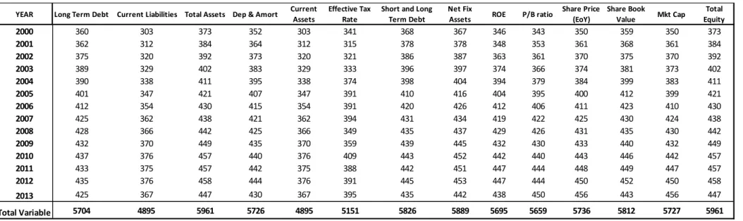
Table 1 present the overview of the data collected from Bloomberg used to build the model variables as its completeness of information for each year and variable. In the table we can see a total number of observations of 78.637.
Figure 1 and Figure 2 present the distribution of observations across the years and across variables. The figures suggest homogeneity and completeness of data.
Considering the most relevant existent literature about debt maturity, we set seven firm-specific variables to use in our model. These are: Debt Maturity (the dependent variable), Growth Options, Firm Quality, Asset Maturity, Liquidity, Firm Size and Effective Tax Rate.
14 Description from www.stoxx.com.
15
12
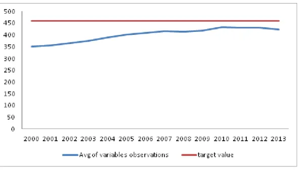
Table 2 presents the overview of the data firm-specific variables to use in the model with a 39,215 total number of observations. Good data base completeness and consistency result would be the number of observations per year close to the number of firms (460) for each variable. This overview is complemented by the Figure 3 which shows graphically the disparity of each year for the target value of observations 460. The value of observations for each year is the average of the number of observations across all the variables considered in our model for its respective year.
It is possible to see that further into to the time we move, more observations we have for each variable in average.
Figure 4 shows the number of observations by each variable. It is easy to observe that
Liquidity and Effective Tax Rate are the ones that have fewer observations when compared
with the other variables.
We consider that the data base and the variables built from it are in equilibrium in terms of distribution of observations and provide a strong balanced and robust data base to run the model and consequently to get solid estimates. The impact of missing data or other lack associated to data base quality is not an issue.
In this work was decided not to clean the extreme outliers of the observations for the simple reason that the quality and robustness of data base is strong and lead us to accept the values as they are, even if the extreme values may drive our estimates to unexpected values (which is not the case). Even though frequency distribution of observations for each firm specific variable was performed to infer about the extreme outliers and their impact on the overall estimates results. In conclusion, the extremes observations are not significant, i.e. they do not occur frequently. Also, cleaning outliers may reduce the quality of the data base as we are reducing its size.
3.2 Firm-Specific Variables Dependent Variable
Debt Maturity. The dependent variable is the maturity of debt. This variable was differently
measured across the authors of several studies. Guedes and Opler (1996) proxy it as maturity of issued bonds, Barclay and Smith (1995) as a percentage of debt that matures after a chosen period and Stohs and Mauer (1996) as a weighted average of all debt obligations. In this hesis
13 we proxy debt-maturity as the maturity that is due beyond 1 year (Long term Debt) to Total Debt (Short and Long Term Debt) as Barclay and Smith approach.
Independent Variables
Growth Options. Used in many relevant works about the topic as Guedes and Opler (1996),
Barclay and Smith (1995) and Stohs and Mauer (1996), the Market-to-Book ratio is a proxy for growth opportunities The ratio is computed as market value of assets, divided by the book value of assets. The market value of assets is determined by the book value of assets, less the book value of equity, plus the market value of equity. If the Market-to-Book ratio is higher than one, i.e. if the market value of its assets is higher than book value it might be expected to have profitable investment opportunities.
According to Myers (1977) and (Myers and Majiluf, 1984), the growth opportunities affect the debt maturity structure decision due to the underinvestment problem, that can be minimized by issuing short-term debt. Thus, Market-to-Book ratio is expected to have a negative coefficient.
Firm Size. Firm size is measured as natural log of the market value of total assets. In Guedes
and Opler (1996) work the authors provide a table16 that shows a summary of empirical predictions using several proxy variables resulting in a positive/negative relation. Regarding the firm size variable the table shows a positive relation between agency costs (underinvestment and asset substitution problem), and negative relation with liquidity risk. The coefficient is expected to be positive.
Firm Quality. The asymmetric information and signalling hypothesis state that managers and
insiders have more privileged information about the value of the firm and its projects than the outsiders and as Flanery (1986) suggested in his work, high (low) quality firms with favourable private (unfavourable private) information tend to signal their quality by issuing short-term (long-term) bonds. We use as a proxy for Firm quality the return on equity (ROE). The coefficient sign is then expected to be negative.
Asset Maturity. As a proxy and following Stohs and Mauer (1996) approach, asset maturity is
measured as the ratio of Gross property, plant and equipment (Fixed Assets) to depreciations and amortizations. As the asset and debt maturity matching hypothesis suggests, the debt
16 Guedes, J. and T. Opler (1996), The Determinants of the Maturity of Corporate Debt Issues, The Journal of
14 maturity tend to be settled to match asset maturity to face its due liabilities. Hence, it is expected a positive sign for the coefficient.
Effective Tax Rate. The effective tax rate is computed as a ratio of Firm’s Total Taxes paid to
firm´s pre-tax income. The higher the tax rate, the greater is the incentive to issue debt to get tax-shields. Either positive or negative coefficient can be expected as the fiscal systems across countries vary and consequently the deductibility of interests from debt. Also even if assuming constant fiscal scenario across countries, deductible interests from financing positive relate to debt issuance, not distinguish from short or long term maturities.
Liquidity. Diamond (1991) argues that by financing with short-term debt firms could face
problems of lack of liquidity in the future, since the cash flows generated may not be sufficient to meet the present obligations of the firm or the maturity of the assets are overset on the long term. Firms with high liquidity levels are expected to have more long term debt. The liquidity variable is computed as the ratio of current assets to current liabilities. A positive coefficient is expected.
15 4. Methodology
In this section is presented the methodology to be used, the description of each econometric model and the rational behind them to support our conclusions.
Our database configures as bi-dimensional data base, as in the first dimension “i” represents the firms and the second dimension “j” represents years. This let us to define our firm-specific variables as Xij. This kind of database configuration leads us to define our analysis as time
series cross-sectional analysis (TSCS), a.k.a. panel data analysis, or longitudinal database analysis. Being so, this database analysis method allows us to take advantage of a particular characteristic: the unobserved information effects. They are the cross sectional information among the firms “i”, and the time-series information reflected within firms over time “j”, as there is constant number of “j” for each “i”.
With Panel Data we are able to control the unobservable variables by observing changes in dependent variable over time. A good example is the Europe GDP, or Europe CPI, or EUR 10-y Bond Yield. These examples are quite good ones given our database of firms from STOXX Europe 600 and the fact that they vary across time but are constant among firms. But we can also explore the effects of variation through firms, or even both simultaneously by using different regression models: firm/time fixed effects models, random effects model or between effects model.
To define our appropriate regression model we must infer about some assumptions behind the models used in the main literature about Debt Maturity topic: the OLS Regression. The OLS is probably the most common estimation model used to regress variables, but when using Panel Data, maybe some assumptions are being violated (Stimson1985, Hicks 1994, Beck and Katz 1995, 1996). The main assumptions are the homoschedasticity17 and the independence of the errors.
In this work, the statistical and econometric tests are performed with STATA software.
In order access the statistical significance of unobservable individual effects we proceed with the Breusch and Pagan Lagrangian Multiplier test (or LM test), which tests the null hypothesis of the unobservable effects are not significant to explain dependent variable
17 Homoschedasticity is a statistical term used to name situations where the variance of the errors (random
16
against the random effects. We reject the null (X2 (1) = 3598.29; p<0.0000), then, we reject the pooled regression hypothesis and we affirm that OLS regression is not the best model to use and we assume the presence of unobservable individual effects.
Then we run the Hausman test to choose between random effects regression or fixed effects regression. The Hausman test tests the null hypothesis that the coefficients estimated by the efficient random effects estimator are the same as the ones estimated by the consistent fixed effects estimator. We reject the null where the random effects regression would be more appropriated and we conclude that the fixed effects model is the most appropriated model (X2 (6) = 116.11; p<0.001).
Given these results we decided to run 4 models in order to access and explore the impact of unobservable effects through different approaches.
The generalized regression mathematical expression for fixed effects (1) and random effects (2) presents as follows:
Yij = β0+β1X1,ij+…+βkXk,ij+ү2E2+…+үnEn+δ2T2+…+δjTj+uij1819 ; (1) Yij = β0+β1X1,ij+…+ βkXk,ij+ uij+
ε
ij20 ; (2)Where:
Yij is the dependent variable (debt maturity), with i=entity and j=time. X1,ij represent the independent variables (determinants).
βk is the coefficient for independent variables. uij is the error term; (between-entity error for RE)
18 “The key insight is that if the unobserved variable does not change over time, then any changes in the dependent variable must be due to influences other than these fixed characteristics”. Stock and Watson, 2003, p.289-290.
19 “In the case of time-series cross-sectional data the interpretation of the beta coefficients would be
…for a given country, as X varies across time by one unit, Y increases or decreases by β units”
Bartels, Brandom, “Beyond “Fixed Versus Random Effects”:” A framework for improving substantive and statistical analysis of panel, time-series cross-sectional, and multilevel data”, Stony Brook University, working paper, 2008).
20 “…the crucial distinction between fixed and random effects is whether the unobserved individual effect
embodies elements that are correlated with the regressors in the model, not whether these effects are stochastic or not” [Green, 2008, p.183]
17
En is the entity n. Since they are binary (dummies) we have n-1 entities included in the
model.
ү2 is the coefficient for the binary regressors (entities).
Tj is time as binary variable (dummy), so model has t-1 time periods. δj is the coefficient for the binary time regressors.
εij is the within-entity error
The models are specified as:
Model 1 – Firm Fixed Effects Regression Model.
This model allows us to control the unobserved effects that differ among firms but are constant over time. Our goal here is estimate coefficients assuming unobservable effects vary across firms and are constant across time, i.e. firm specific characteristics that impact debt maturity.
Model 2 – Industry Fixed Effects Regression Model
Similar to the Model 1, this model allows us to estimate the coefficients assuming now individual industry characteristics.
Model 3 – Time Fixed Effects Regression Model
In this model we control unobserved effects that differ over time but are constant across firms. Exogenous factors that vary with time and are constant over firms could be GDP, CPI, 10y Bond Yield, among others. Our goal is see if changes in debt maturity were impacted by exogenous factors that vary over time.
We also set a dummy variable (YR1) for period analysis as it takes a value of 0 for years 2000 to 2007 and value of 1 for years 2008 and ahead, in order to compare the coefficients before and after 2008 subprime crisis.
Model 4 – Random Effects Regression Model
We believe exogenous variables’ effects are constant over time and vary across firms, and other may vary over time and be constant across firms, thus, random effects model allows us to control for this. GLS regression to random effects was performed in this model.
18
All the estimated regressions were included heteroskedasticity-robust standard errors (a.k.a. Huber/White estimators) and cluster option21 to deal with heteroskedasticity22 (or no homoschedasticity) and autocorrelation, respectively.
Descriptive statistics and correlation coefficients matrix are also performed in this work allowing for a better comprehension of the behaviour and relationship among the variables.
21 STATA option to deal with autocorrelation among the panel variables.
22 Heteroskedasticity is a statistical term used to describe non-constant variance among the estimated regression
19 5. Empirical Results and Discussion
In this section are presented the results of the debt maturity analysis. Different analysis/approaches were developed in order to describe the behaviour of debt maturity and the relevance of its determinants by different models and sample periods. Descriptive statistics, correlation matrix and different regression models were performed and the results are described further on this chapter.
5.1 Descriptive Statistics Analysis
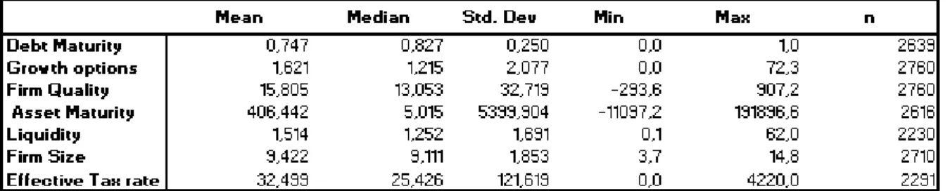
Table 3 and, Table 4 and Table 5 report the descriptive statistics of the dependent and independent variables used for the period 2000-2013, 2000-2007 and 2008-2013, respectively.
Regarding Debt Maturity for the whole period, the average percentage of debt maturing after one year is 70.5%, below its median value of 78.9%. The standard deviation of its values is 26.75 pp. For 2000-2007 period the average and median value are 67.1% and 74.9%, respectively, while, for the 2008-2013 period the average and the median value are 74.7% and 82.7%, respectively. These values suggest an increase of debt maturity ratio from period before subprime crisis to the period after. The standard deviation is higher for 2000-2007 period (27.7pp) than for 2008-2013 period (25pp).
Given these results we might be present an upward trending in the level of the debt maturity. Table 6 and Figure 5 show the evolution of the debt maturity levels across the whole sample period, and the upward trend seems to be a fact.
20
Figure 5 - Debt maturity ratio trend for whole sample.
In 2000 the mean level of debt maturity is 59.41% and in 2013 is 75.8%, representing an increase around 16pp. An interesting observation is that the highest variation on debt maturity level is from year 2008 to 2009, almost 4pp.
To better understand this fact, a more detailed analysis is needed, since there are multiple ways of proxy debt maturity. The proxy to debt maturity level used in this work is the proportion of debt that matures beyond one year of the total debt. Figure 6 presents the evolution of Short-term debt, Long-term Debt and Total Debt23, where is possible to observe the break on an strong upward trend to a flat trend in Long-term debt in 2008, and also a break on the Short-term debt trend in 2007 to a further downtrend to lowest levels of the sample.
23
21
Figure 6 - Decomposition of Total Debt evolution by short and long-term debt across whole sample years.
The upward trend on debt maturity level is then caused by a decreasing preference for short-term debt regarding the post subprime period, rather than the increasing of levels of total debt in firm’s balance sheet as seen in period before the subprime.
Concluding, after 2008, firms are optimizing their levels of debt maturity by decreasing slightly the total amount of debt, as seen the break of the upward trend in Total Debt in 2008 (Figure 6), and they are financing themselves through long-term debt rather short-term debt.
Regarding the independent variables their averages and median values remain almost the same for all periods and sub-periods with exception for the Asset Maturity variable which report a significant decrease of a roughly 50% of its value from 2000-2007 to 2008-2013 period. A possible reason for that could be that firms did not invested in new assets, and depreciations kept going on over those assets.
Figure 7 and Table 7 present the evolution of Debt Maturity clustered by industry sector. This graph presentation provides an analysis that highlights the differences in the debt maturity levels by industry sectors along the whole period. Telecommunication services is the sector who presents highest Debt Maturity ratio before 2008, while Consumer staples presents the lowest, in average terms. A convergence to the same level of Debt Maturity ratio among all sectors is observable further we move to the end of the sample period. It is possible to see in Figure 7 that in the first years of the sample the Debt Maturity ratios were spread wide, meaning that the levels of the ratio were significantly different across sectors. But looking to the period after 2008, the Debt Maturity ratio seem to be converging to a
22
narrow interval between 70% and 80% suggesting an optimizing structure of debt maturity into firm’s balance sheets.
5.2 Correlation Analysis
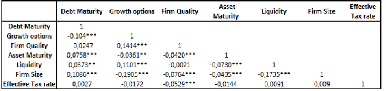
In this section is analysed the correlation coefficients among the variables. Simple correlation method was performed at 99%, 95% and 90% confidence level. Table 8 presents the correlation matrix for the variables.
Table 8 - Correlation matrix.
Only Growth Options (-0.104), Asset Maturity (0.00768) and Firm Size (0.1086) have significant coefficients at 99% level when correlated with Debt Maturity, while Liquidity (0.0373) is significant at 95%. Effective tax rate and Firm Quality have not significant coefficient at any level performed. Their signs are in accordance with the expected and they are similar to those later found in regression analysis. The two strongest coefficients are between Firm Size and Liquidity 0.1735) and between Firm Size and Growth Options (-0.1905), both significant at 99% level, suggesting negative relation between size, liquidity and growth options. Given the low correlation coefficients among the variables the regression models performed will not have multicollinearity problems.
5.3 Regression Analysis
In this section are presented the results and interpretation of the coefficients across all regression models and also the comparison among them. Argumentation and possible explanations for the results are made to address coefficients importance through data sample to explain Debt Maturity trend. All the arguments are supported by the most relevant findings in the literature and support analysis specifically performed for the purpose24. Comparison
24
23
between different periods (pre-subprime and post-subprime) is performed to address the change in importance of coefficients to explain the dependent variable.
5.3. 1. Analysis of determinants
Presenting the equation of Model 3 for whole sample period, the Time Fixed Effects Regression:
Debt Maturityij = 0.5915 – 0.0086Growth Optionsij – 0.00008Firm Qualityij + 0.000023Asset
Maturityij + 0.0187Liquidityij + 0.0134Firm Sizeij + 0.000004Eff Tax Rateij + δjTj+uij ;
All the coefficients are statistically significant at the 1% level (p<0.01) with the exception of Firm Quality and Effective Tax Rate which are not statistically significant.
Table 9 presents the coefficients for all regression models performed. P-values are also presented to observe the statistical significance of coefficients at 1%, 5% and 10% levels.
Adjusted R-squared is presented at the bottom of the table.
24
According to the results of most relevant academic literature on Corporate Finance theme, the expected signs for the coefficients of the determinants are as follows:
Table 10 - Expected signs of the determinants of Debt Maturity. Independent Variables Expected signs of coefficients Growth options +/-Firm Quality Asset Maturity + Liquidity -Firm Size +
Effective Tax rate
+/-The signs of the coefficients presented in Table 9 are aligned with the expected signs from the table above, with the exception of liquidity, which shows positive signs across all models, but this issue is discussed further in this section.
Next is presented the analysis of determinants addressing its relevance across all models.
Growth Options – presents a negative relation and statistical significance at 1% level (p<0.01) across all models except in Model 1 that is statistically significant at 5% level (p<0.05). Comparing firm and time fixed effects regression (Model 1 and Model 3, respectively) for whole period, in Model 1, the coefficient presents a value of -0.0046 meaning that in average, an increasing in firms’ growth options ratio of 1pp leads to a decrease of 0.0046pp in debt maturity ratio. Looking to Model 3 we can see a stronger coefficient, meaning that in average, an increasing in firm’s growth options ratio of 1pp leads to a decrease of 0.0086 pp in debt maturity ratio. This result is consistent with the agency costs theory where increasing opportunities to growth should lead to shorter debt maturity ratios. On other hand, these results do not support the liquidity risk argument suggested by Diamond (Diamond, 1991a) where firms issue long term debt to avoid inefficient liquidation of riskier growth options.
The value of coefficient, or the estimated impact on debt maturity of Growth Options, has its high values in Model 2 (-0.009) and Model 3 (-0.0085) for whole sample period. But we can denote a huge increase on its importance when compared with sub-period 2008-2013 in Model 3 presenting a value of -0.026. This result suggests an increase of its importance after subprime crisis in driving debt maturity across firms.
25
Firm Quality – presents mixed signs on its coefficient and is not statistically significant at any level in any model.
Signaling hypothesis suggests that firms with higher future earnings tend to issue more short-term debt to signal its quality to the market. Although, poor results on this deshort-terminant show that its relevance is week. Other authors also found poor results to this theory, like Ozkan (2000), Antoniou, Guney and Paudyal (2006) and Dennis et al. (2000).
A possible explanation for the obtained results is, like Diamond (1991) suggest, a non-monotonic relationship between debt maturity and firm’s quality may exist, since low and high quality firms choose both short-term debt and medium quality firms opt for long-term debt.
Other explanations could be high quality firms rather prefer a combination of short and long term to avoid inefficient liquidation and, since the Stoxx EUR 600 Index firms are all quoted the asymmetry of information may not be relevant as they are required to constantly realize information to the market they cannot simply pretend its quality through issuance of short term debt.
Asset Maturity – presents positive relation and the coefficient is statistically significant at 1% level in all models with exception the Model 1 where it presents a negative sign but not significant at any level. In general the results are in accordance with the expected and the matching theory between assets and debt maturity finds good support. Among all statistical significant coefficients across all models, Model 3 shows that for the 2000-2007 period the coefficient has the highest value (0.0000342) and 2008-2013 has the lowest (0.0000126) suggesting a decrease of its importance after subprime crisis.
Liquidity – presents positive relation and it is statistically significant at 1% level across all models with exception in Model 3 in 2008-2013 period which is not significant.
For the whole period, Model 1 and Model 4 present the strongest coefficient, 0.078 and 0.065, respectively.
In spite of strong coefficients on this determinant and their statistical significance, they present a contrary sign to the expected. A possible explanation for this contrary sign could be related to non-specific firm features, i.e. macro-economic variables like interest rate term structure volatility. Increasing short-term interest rates volatility could have changed firm’s decisions to finance through long-term debt instead short-term. Even for the high liquidity firms the benefits of cheaper short term financing (or roll over strategies) could not
26
compensate the risk of uncertainty of short term rates in the close future. In Model 3, the coefficient for liquidity in the period 2008-2013 becomes extremely irrelevant to explain debt maturity presenting a P-Value of 0.474 and reduces its value almost seven times when compared to 2000-2007 period. This fact corroborates with the observed increasing volatility on the short-term interest rates after 2007 subprime crisis. Figure 8 (appendix 2) present the evolution of volatility of yield curve interest rates from Euro Zone AAA (spot rates) between 2004 and mid-2014.
Firm Size – presents positive relation and statistically significant coefficient at 1% level across all models being aligned with the expected results found in literature where is shown that large firms tend to have more long-term debt in their debt maturity structure due to low levels of asymmetry and agency problems. Model 1 has the highest coefficient among all models (0.0835). For the whole period Model 1 has a much higher coefficient than Model 3 suggesting unobservable firm specific features explain more the dependent variable than unobservable time specific effects regarding Firm Size variable. Model 3 show us that the relevance of the determinant has decreased from 2000-2007 (0.0135) to 2008-2013 (0.0105) period.
Effective Tax Rate – presents mixed signs on its coefficients and not statistical significance in any model at any level.
Similar to our results, like Ozkan (2000, 2002) findings, effective tax rates do not produce any impact in debt maturity ratios. Antoniou, Guney and Paudyal (2006) also provide similar conclusions for French and English firms. But there are quite different results found in the existing literature about the relevance of this determinant, which could be related to the variety of samples chosen as the fiscal laws are different across countries and industry sectors.
5.4. Final remarks about subprime impact on debt maturity decision
We believe that subprime and its consequences contributed to change the way that debt maturity is driven. In this section are analyzed in more detail the changes in coefficients of determinants between the 2000-2007 and 2008-2013 periods with the intent of wrapping up the main conclusions.
Starting by changes in coefficients statistical significance, only Liquidity determinant lost its significance from one period to another (period 2000-2007: P-value (<0.001) and period 2008-2013: P-value (0.474)). All other coefficients from the determinants kept their
27
significance. A possible explanation for this fact was already addressed in the section above where it is attributed the increasing volatility on short-term interest rates after 2007 as the main factor to drive firm’s decision to finance through long-term debt in substitution of short-term debt, contributing to offset the relevance of Liquidity factor in explaining Debt maturity.
Regarding the values of coefficients, (i.e. their level of impact on debt maturity) the coefficient of Liquidity reduced its value by seven times from period 2000-2007 (0.0326) to period 2008-2013 (0.0047). An increase rounding 300% in Growth Options coefficient is observed from pre-subprime to post-subprime period, both statistically significant at 1% level, suggesting that this determinant became more important to explain the behavior of debt maturity after 2007.
Asset Maturity shows decreasing value on its coefficient by almost 200% from pre-subprime period to post. Firm size determinant reduces its coefficient by 26% from 2000-2007 (0.0135) to 2008-2013 (0.0105) period.
In general, Growth Options increases its importance, while Liquidity, Asset Maturity and Firm Size lost importance in terms of impacting debt maturity behavior. This is consistent with the macro-economic happenings derived from subprime crisis in 2007, where other factors beyond firm-specific determinants had increasing importance to explain debt maturity structure. This can also be confirmed by comparing the Adjusted R-squared25 between
2000-2007 and 2008-2013 periods, where it decreases from 0.0462 to 0.0318, respectively.
25 Adjusted R-squared measures how much the model variables explain the dependent variable, i.e. the quality of
28
SUMMARY OF DESCRIPTIVE STATISTICS
Table 3 - Descriptive Statistics of firm specific variables for whole period (2000-2013)
Table 4 - Descriptive Statistics of firm specific variables for sub-period (2000-2007)
Table 5 - Descriptive Statistics of firm specific variables for sub-period (2008-2013)
29
30
Figure 7 - Debt Maturity Levels for whole sample by Industry Sectors.
0 0,1 0,2 0,3 0,4 0,5 0,6 0,7 0,8 0,9 2000 2001 2002 2003 2004 2005 2006 2007 2008 2009 2010 2011 2012 2013 Consumer Discretionary Consumer Staples Energy Health Care Industrials Information Technology Materials Telecommunication Services Utilities
31 6. Conclusion, limitations and further research
The results of this empirical work seem to be aligned with the most relevant academic works on debt maturity scope. The models used in our methodology and the specific purpose analysis performed provide plausible evidence to support the conclusions presented.
It is straightforward to observe that Debt Maturity ratio has an increasing behavior over our sample. At the beginning of the sample, in year 2000, the value of this ratio is in average 59.41%, while at the end, in year 2013, this ratio has a value of 75.8%. In the first four years of our sample (2000-2004) this ratio increased 11 pp to a value of 70.4% (2004), marking this period as the one who had a faster pace on the increasing behavior of Debt Maturity.
The analysis suggests that after 2007 there was a change in the structure of debt into firm’s balance sheets where firms started to replace short-term debt for long-term debt. This preference might be explained by the highest levels of volatility regarding short-term interest rates after 2007 as suggested in the specific purpose analysis performed on Yield Curve Euro Area AAA. Facing this short-term interest rate volatility scenario, firms avoided interest rate risk on their short-term financing strategies by financing through long-term debt. Nevertheless, the behavior of Debt Maturity ratio kept increasing.
The determinants of Debt Maturity used in this work have the expected signs observed from the main literature and empirical works on this scope with exception for Liquidity, where the sign is positive across all models being in discordance with liquidity theory that states that high liquidity firms tend to issue short-term debt maintaining their Debt Maturity ratio low. Sharp (1991) suggests that borrowing long-term avoid inefficient liquidation risk, and this could be one plausible reason even for high liquidity firms borrow long-term.
Regarding the impact of subprime crisis on Debt Maturity firm specific drivers, our analysis suggests that Liquidity become irrelevant to explain Debt Maturity after 2007, whereas Growth Options increased significantly its power after subprime. Our results also suggest that other factors beyond firm specific ones, i.e. macro-economic factors, became more important to explain Debt Maturity ratio after 2007.
In general, STOXX EUR 600 Index’ firms are now holding more debt in their balance sheets than they were at the beginning of new millennium, but a preference for long-term debt rather than short-term debt is been seen since the subprime crisis in 2007 leading to an optimization of debt maturity structure.
32
Naturally, are identified some limitations on this work. The methods used to proxy and measure the determinants are a good example, as we measure Debt Maturity ratio as the proportion of debt that matures after one year, or Firm Quality measured by ROE might not be the best proxies to use. Also, we only use firm specific determinants in our models to explain the dependent variable, known that macro-economic determinants are also important to describe Debt Maturity behavior.
In the near future credit market may suffer some changes and become more challenging for firms. Basel III regulations on financial institutions regarding liquidity risk bring up some ratios to be implemented in 2015 known as LCR26 and further others like NSFR27. These ratios have minimum targets to be achieved and as part of this, the Banks are required to improve the quality of capital by investing in HQLA (high quality liquid assets) and to seek for more stable sources of funding. An immediate consequence would be less available capital to invest in corporate bond market that pays a higher yield than government bond market. Corporate firms are about to find more difficult in the near future to finance themselves by simply issuing debt or borrow from banks as they are accustomed. This fact could be important in the future regarding credit market and how the financial market will figure a solution to respond to the firm’s need of capital. Given the importance and role of banks in the economy, an interesting theme for further research could be how are related financial institution’s liquidity management and corporate firm’s debt maturity.
26 Liquidity Coverage Ratio
27
33 Bibliographic References
Barclay, M. and C. Smith (1995), The Maturity Structure of Corporate Debt, The Journal
of Finance 50, Issue 2, 609-631.
Barnea, A., R. A. Haugen and L. W. Senbet (1980), A Rationale for Debt Maturity Structure and Call Provisions in the Agency Theory Framework”, The Journal of Finance 35, Issue 5, 1223-1234.
Bartels, Brandom, “Beyond “Fixed Versus Random Effects”: A framework for improving substantive and statistical analysis of panel, time-series cross-sectional, and multilevel data”, Stony Brook University, working paper, 2008.
Brick, I. and S. A. Ravid (1985), On the Relevance of Debt Maturity Structure, The
Journal of Finance 40, Issue 5, 1423-1437.
Brick, I. and S. A. Ravid (1991), Interest Rate Uncertainty and the Optimal Debt Maturity Structure, Journal of Financial and Quantitative Analysis 26, Issue 1, 63-81.
Diamond, D. (1991a), Debt Maturity Structure and Liquidity Risk, Quarterly Journal of
Economics 106, Issue 3, 709-737.
Elaine Harwood and Gil B. Manzon, Jr., (2000), Taxes Clienteles and Debt Maturity, The Journal of American Association Taxation, 22-39.
Flannery, M. (1986), Asymmetric Information and Risky Debt Maturity Choice, The
Journal of Finance 41, Issue 1, 19-37.
Franco Modigliani and Merton H. Miller (1958), The Cost of Capital, Corporation Finance and the Theory of Investment¸The American Economic Review, Vol. 48, No. 3 (Jun., 1958), pp. 261-297
Franco Modigliani and Merton H. Miller (1963), Corporate Income Taxes and the Cost of Capital: A Correction, The American Economic Review, Vol. 53, No. 3 (Jun., 1963), pp. 433-443
Guedes, J. and T. Opler (1996), The Determinants of the Maturity of Corporate Debt Issues, The Journal of Finance 51, Issue 5, 1809-1833.
Junesuh Yi, (2005), A Study on Debt Maturity Structure, Journal of American Academy of Business, Cambridge, 277-285.
Kraus, A. and R. Litzenberger (1973), State Preference Model of Optimal Financial Leverage, The Journal of Finance 28, Issue 4, 911-922.
Leland, H. E. and K. B. Thoft (1996), Optimal Capital Structure, Endogenous Bankruptcy, and the Term Structure of Credit Spreads, The Journal of Finance 51, Issue 3, 987-1019.