Government spending efficiency, measurement and applications : a cross-country efficiency dataset

(1)

REM WORKING PAPER SERIES

Government Spending Efficiency, Measurement and

Applications: a Cross-country Efficiency Dataset

António Afonso, João Tovar Jalles, Ana Venâncio

REM Working Paper 0147-2020

November 2020

REM – Research in Economics and Mathematics

Rua Miguel Lúpi 20,

1249-078 Lisboa, Portugal

ISSN 2184-108X

Any opinions expressed are those of the authors and not those of REM. Short, up to two paragraphs can be cited provided that full credit is given to the authors.

(2)

REM – Research in Economics and Mathematics

Rua Miguel Lupi, 20 1249-078 LISBOA Portugal Telephone: +351 - 213 925 912 E-mail: rem@iseg.ulisboa.pt https://rem.rc.iseg.ulisboa.pt/ https://twitter.com/ResearchRem https://www.linkedin.com/company/researchrem/ https://www.facebook.com/researchrem/

(3)

1

Government Spending Efficiency,

Measurement and Applications: a

Cross-country Efficiency Dataset

*

António Afonso

$

João Tovar Jalles

#

Ana Venâncio

#

November 2020

Abstract

This chapter conducts a review of the literature dealing with overall public sector performance and efficiency, it defines a methodology to assess public sector efficiency and it creates a novel and large cross-sectional panel dataset of government indicators and public sector efficiency scores. The focus is on a balanced sample covering all 36 OECD countries over the time period between 2006 and 2017. First, we define a set of economic and sociodemographic metrics necessary to construct performance composite indicators. Second, we calculate and report a full set of (input and output oriented) efficiency scores based on the performance indicators previously computed.

JEL: C14, C23, H11, H21, H50

Keywords: government spending efficiency, public sector performance, non-parametric estimation, DEA, OECD

*_{The authors acknowledge support by the FCT (Fundação para a Ciência e a Tecnologia) [grant numbers} UIDB/05069/2020 and UIDB/ 04521/2020. The opinions expressed herein are those of the authors and not necessarily those of their employers. This is a draft version of a chapter to appear in the Handbook on Public Sector Efficiency, published by Edward Elgar Publishing.

$_{ISEG, Universidade de Lisboa; REM/UECE. Rua Miguel Lupi 20, 1249-078 Lisbon, Portugal. email:}

aafonso@iseg.ulisboa.pt.

#_{Instituto Superior de Economia e Gestão (ISEG), Universidade de Lisboa, Rua do Quelhas 6, 1200-781 Lisboa,} Portugal. Research in Economics and Mathematics (REM) and Research Unit on Complexity and Economics (UECE), ISEG, Universidade de Lisboa, Rua Miguel Lupi 20, 1249-078 Lisbon, Portugal. Economics for Policy and Centre for Globalization and Governance, Nova School of Business and Economics, Universidade Nova de Lisboa, Rua da Holanda 1, 2775-405 Carcavelos, Portugal. IPAG Business School, 184 Boulevard Saint-Germain, 75006 Paris, France. Email: joaojalles@gmail.com

#_{ISEG, Universidade de Lisboa; ADVANCE/CSG. Rua Miguel Lupi 20, 1249-078 Lisbon, Portugal email:}

(4)

2 1. Introduction

A country´s performance is, in part, dictated by the size of its public sector and the efficiency level with which it uses its (typically scarce) resources.1 It is, therefore, important from both an economic and policy points of view to evaluate the performance of the public sector and understand the determinants of public sector efficiency so as to maximize welfare but also to optimize investment projects and, in that way, propel growth forward. There has been an ongoing debate in the literature over the role and size of the government (Afonso and Schuknecht, 2019), mostly motivated by the substantial heterogeneity across countries in terms of the government spending.2 This issue is even more relevant when governments face strict government budget constraints and most western economies are living in the secular stagnation phase for several years now, notably in the context of economic downturns and of scarce public resources.

In this chapter, we do a systematic review of the literature dealing with the overall public sector performance and efficiency, we define a methodology to compute public sector efficiency and we create a novel and large cross-country panel dataset of government indicators and public sector efficiency scores. We cover a sample of 36 OECD countries over the 2006-2017 time period. More specifically, firstly, we start by defining a set of economic and sociodemographic metrics and we construct composite performance indicators. Previous papers on this topic have typically studied a very limited number of countries over a one or two-year time span, which is a gap we are trying to cover with this work. Secondly, we compute and report a full set of (input and output oriented) efficiency scores on the basis of the performance indicators previously calculated, relating performance outputs and input measures of government spending.

The remainder of the chapter is organized as follows. Section 2 reviews the relevant literature. Section 3 presents some of methods used to obtain public sector efficiency measures. Section 4 discusses recent empirical applications. The last section concludes.

1_{The analysis of the government size with respect to the economic growth has recently received a larger attention of} empirical analysis. The existence of a relationship between the both variables was firstly postulated by the German political economist Adolph Wagner (1911). Lamartina and Zaghini (2011) provided empirical evidence for a positive relationship between government size and GDP per capita using panel of 23 OECD countries.

2_{The government intervenes in the economy in four ways (Labonte, 2010). First, it produces goods and services, such} as infrastructure, education, and national defense. Second, it transfers income, both vertically across income levels and horizontally among groups with similar incomes and different characteristics. Third, it taxes to pay for its outlays, which can lower economic efficiency by distorting behavior. Finally, government regulation alters economic activity.

(5)

3 2. Literature Review

The efficient provision of services and goods by governments has become one of the key issues discussed in the public finance literature in the last 20 years (see for example the works by Gupta and Verhoeven, 2001; Tanzi and Schuknecht, 1997, 2000; Afonso et al., 2005).

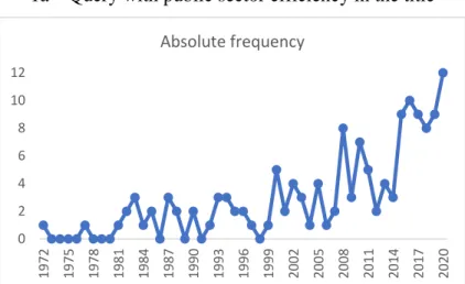
In this section, we review the main studies on public sector efficiency by applying the following methodology. We search the Web of Science3 for English language articles published after 1970 in academic, peer-reviewed journals. To identify relevant publications, we searched for works using two queries: i) with “public sector efficiency” in the tile, and ii) with “public sector” or “efficiency” in the title and “public sector efficiency” in the title, text, abstract, or keywords. The exact search strings were: i) TI = (public sector efficiency) and ii) ALL = “public sector efficiency” AND TI = (public sector OR efficiency). As a result of the search, a total of 142 and 55 articles were identified for queries i) and ii) respectively. Then, we screened these articles to evaluate the topic fit and eliminated those that evaluated local government performance and the performance of a specific public service provided by the local and central governments.4 In doing this, we also evaluated the study subject, research question and findings.

Figure 1 shows the number of publications published per year, using both sets of queries. We observe an increasing trend in publications since 2000, with peaks in the period 2008-2010 and in the period 2019-2020. This reflects the growing interest of academic research in this particular area, which may have been prompted notably by the fiscal institutional setup, for example, in the EU. Indeed, after the creation of the Economic and Monetary Union in the EU in the early 1990s, accrued fiscal coordination and surveillance ensued, with increased awareness of the relevance of fiscal sound behaviour. In addition, the driver and the need to implement fiscal consolidations in the EU (due to convergence criteria needed to be met) raised the bar in terms of assessing how much and what quality of public services are the government providing, while economic crisis also

3_{The Web of Science was chosen as it represents one of the major academic search engines in social sciences and} facilitates a wide-ranging identification of relevant publications.

4_{Within the public sector literature, some studies has evaluated government performance of a specific government} function or the performance of local governments. In terms of local governance performance, see for instance Van den Eeckaut et al. (1993), De Borger et al. (1994) and De Borger and Kerstens (1996, 2000) for Belgium; Athanassopoulos and Triantis (1998) and Doumpos and Cohen (2014) for Greece; Worthington (2000) for Australia; Prieto and Zofio (2001), Balaguer-Coll et al. (2002) and Benito et al. (2010) for Spain; Storto (2015) for Italy; Waldo (2001) for Sweden; and Sampaio and Stosic (2005) for Brazil. In Portugal, we highlight the studies of Afonso and Fernandes (2006, 2008), Afonso and Scaglioni (2007), Cruz and Marques (2014) and Afonso and Venâncio (2016).

(6)

4

shed attention of the use of scarce public resources. Hence, both performance and efficiency started playing a bigger role in the 2000s in the EU case.5

Figure 1 – Yearly publications on the topic of Public Sector Efficiency in Web of Science 1a – Query with public sector efficiency in the title

1b – Query with public sector efficiency in the title, text, abstract and keywords

Source: Web of Science and own elaboration.

5_{“The need to improve competitiveness, concerns about fiscal sustainability and growing demands by taxpayers to} get more value for public money as well as the need to reconsider the scope for state intervention in the economy has prompted efforts to increase the focus of budgets on more growth-enhancing activities and gear the tax mix and the allocation of resources within the public sector towards better efficiency and effectiveness.” (EC, 2007, p. 9).

0 2 4 6 8 10 12 1972 1975 1978 1981 1984 1987 1990 1993 1996 1999 2002 2005 2008 2011 2014 2017 2020 Absolute frequency 0 2 4 6 8 10 12 1983 1985 1987 1989 1991 1993 1995 1997 1999 2001 2003 2005 2007 2009 2011 2013 2015 2017 2019 Absolute frequency

(7)

5

Journals that more frequently show up in the abovementioned sample extractions are Applied

Economics, European Journal of Operational Research, European Journal of Political Economy, Journal of Public Economics, and Public Choice.

Several studies assess public sector efficiency looking at different sample and time spans but most tend to focus on OCDE and European countries (Adam at al., 2011; Duti and Sicari, 2016; Afonso and Kazemi, 2017; Antonelli and de Bonis, 2019). Much less evidence is available about government relative efficiency in other areas of the world such as Africa, Asia or Latin America. That said, some studies report some first empirical explorations for Latin American and Caribbean countries (see e.g. Afonso et al., 2013).

Two key results emerge from this literature: i) public spending efficiency can be improved; and ii) specific factors are associated with efficiency. These cross-country aggregated efficiency studies are very useful to compare the performance of different countries, nevertheless it is important to take into account the underlying institutional, cultural, political and economic factors (Mandl et al., 2008). To account for these issues, studies have resorted to two-stage models.6 Results suggest that education, income level, quality of the institutions and country’s governance are positively and statistically significantly associated with performance (Afonso et al., 2006; Hauner and Kyobe, 2008; Antonelli and de Bonis, 2019). Others report that political variables, such as having a right-wing and a strong government and also high voter participation rates and decentralization of the fiscal systems, are positively associated with more efficient public sectors (Adam et al., 2011). More recently, Afonso et al. (2019, 2020) evaluated the role of tax structures and tax reforms on explaining cross-country efficiency differences. Table 1 provides a short summary of results of these papers assessing overall public sector performance and efficiency.

[insert Table 1]

3. Data and Variables

Our novel data set includes 36 OECD countries7 for the period between 2006 and 2017. We gather data from several publicly available sources, such as World Economic Forum, World

6_{For instance, Ruggiero (2004) and Simar and Wilson (2007) provide an overview of this issue.}

7_{The 36 OECD countries considered are: Australia, Austria, Belgium, Canada, Chile, Czech Republic, Denmark,} Estonia, Finland, France, Germany, Greece, Hungary, Iceland, Ireland, Israel, Italy, Japan, Korea, Latvia, Lithuania,

(8)

6

Bank, World Health Organization, IMF World Economic Outlook and OECD database. When data was not available for a specific year, we assumed that the data was equal to that of the previous year.

Government spending can have many (often-competing) objectives (promoting stability, allocation, and redistribution) and any definition of efficiency must be understood in this Musgravian sense. Following the related literature, we use a set of metrics to construct a composite indicator of Public Sector Performance (PSP), as suggested by Afonso et al. (2005, 2019). PSP is then computed as the average between opportunity and Musgravian indicators.

First, opportunity indicators reflect governments’ performance in the administration, education, health and infrastructure sectors. The administration sub-indicator includes the following measures: corruption, burden of government regulation (red tape), judiciary independence, shadow economy and the property rights. To measure the education sub-indicator, we use the secondary school enrolment rate, quality of educational system and PISA scores. For the health sub-indicator, we compile data on the infant survival rate, life expectancy and survival rate from cardiovascular diseases (CVD), cancer, diabetes or chronic respiratory diseases (CRD). The infrastructure sub-indicator is measured by the quality of overall infrastructure.

Second, Musgravian indicators include three sub-indicators: distribution, stability and economic performance. To measure income distribution and inequality, we use the Gini coefficient. For the stability sub-indicator, we use the coefficient of variation for the 5-year average of GDP growth and the rolling overlapping standard deviation of 5 years inflation rate. To measure economic performance, we include the 5-year average of real GDP per capita, real GDP growth and unemployment rate. Accordingly, both opportunity and Musgravian indicators result from the average of the measures included in each sub-indicator. To ensure a convenient benchmark, each sub-indicator measure is normalized by dividing the value of a specific country by the average of that measure for all countries in the sample. Table 2 lists all sub-indicators to construct the PSP indicators and provides further information on the sources and variable construction.

[insert Table 2]

Luxembourg, Mexico, the Netherlands, New Zealand, Norway, Poland, Portugal, Slovak Republic, Slovenia, Spain, Sweden, Switzerland, Turkey, the United Kingdom, and the United States.

(9)

7

Our input measure, Public Expenditure (PE) is expressed in percentage of GDP and it considers each area of government expenditure. More specifically, we consider government consumption as input for administrative performance, government expenditure in education as input for education performance, health expenditure as input for health performance and public investment as input for infrastructure performance. For the distribution indicator, we consider expenditures on transfers and subsidies. The stability and economic performance are related to the total expenditure. Table 3 includes data on various governments’ expenditures and provides further information on the sources and variable construction.

[insert Table 3]

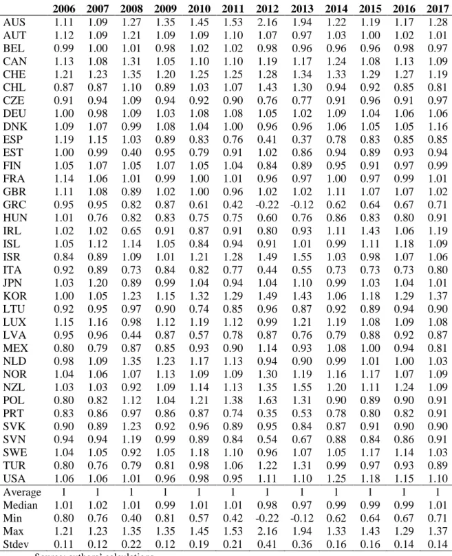
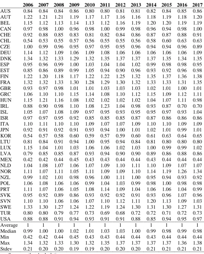
Tables 4 and 5 show the evolution of the standardized PSP and PE indicators, respectively, normalised to one in each year. For instance, the overall dispersion of the PSP indicator, although not too different between 2006 and 2017, increased during the European debt crisis of 2011-2013. Note that Greece presented a negative performance on the stability and economic performance sub-indicators in years 2012 and 2013 and, consequently, the “Musgravian” and the overall PSP score are negatives.

[insert Table 4] [insert Table 5]

4. Methodology

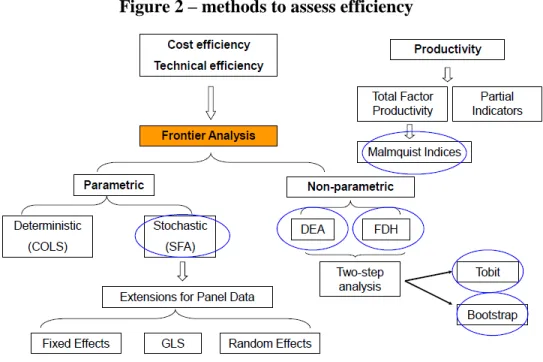
To compute efficiency, previous surveyed papers use several parametric and non-parametric methodologies. Parametric approaches include corrected ordinary least squares (OLS) and stochastic frontier analysis (SFA). Among the non-parametric techniques, data envelopment analysis (DEA) and free disposal hull (FDH) have been widely applied in the literature. Most of the studies estimate a non-parametrically production function frontier and derive efficiency scores based on the relative distances of inefficient observations from the frontier. Figure 2 illustrates some of the possible methods available to assess efficiency.

(10)

8

Figure 2 – methods to assess efficiency

Source: own elaboration.

Following the literature, in order to compute public sector efficiency scores, we use a DEA approach,8 which compares each observation with an optimal outcome. DEA is a non-parametric technique that uses linear programming to compute the production frontier. For each country i out of 36 advanced economies, we consider the following function:

𝑌_𝑖 = 𝑓(𝑋_𝑖), 𝑖 = 1, … ,36 (2)

where 𝑌is the composite output measure (Public Sector Performance, PSP) and 𝑋 is the composite input measure (Public Expenditure, PE), namely government spending to GDP ratio.

In Equation (2), inefficiency occurs if 𝑌_𝑖 < 𝑓(𝑋_𝑖), implying that for the observed input level, the actual output is smaller than the best attainable one.

In computing the efficiency scores, we assume variable-returns to scale (VRS), to account for the fact that countries might not operate at their optimal scale.

8_{DEA is a non-parametric frontier methodology, which draws from Farrell’s (1957) seminal work and that was further} developed by Charnes et al. (1978). Coelli et al. (2002) and Thanassoulis (2001) offer introductions to DEA.

(11)

9

We use two orientations: input and output orientation. The input orientation allows us to measure the proportional reduction in inputs while holding output constant. Using the input approach, efficient scores are computed through the following linear programming problem:

min 𝜃,𝜆 𝜃 𝑠. 𝑡. − 𝑦𝑖+ 𝑌𝜆 ≥ 0 𝜃𝑥_𝑖− 𝑋𝜆 ≥ 0 𝐼1’𝜆 = 1 𝜆 ≥ 0 (3)

where 𝑦_𝑖 is a column vector of outputs, 𝑥_𝑖 is a column vector of inputs, 𝜃 is the input efficiency score, 𝜆 is a vector of constants, 𝐼1’ is a vector of ones, 𝑋 is the input matrix and 𝑌 is the output matrix..

In equation (3), 𝜃 is a scalar (that satisfies 0 ≤ 𝜃 ≤ 1) and measures the distance between a country and the efficiency frontier, defined as a linear combination of the best practice observations. With 𝜃 < 1, the country is inside the frontier, it is inefficient, while 𝜃 = 1 implies that the country is on the frontier and it is efficient.

Conversely the output orientation allow us to measure the proportion increase in outputs holding inputs constant. In this approach, the efficiency scores are computed through the following linear programming problem:

max φ φ,𝜆 𝑠. 𝑡. − 𝜑𝑦_𝑖 + 𝑌𝜆 ≥ 0 𝑥_𝑖 − 𝑋𝜆 ≥ 0 𝐼1’𝜆 = 1 𝜆 ≥ 0 (4)

In equation (4),  is a scalar (that satisfies 1≤  ≤ +∞), and -1 is the proportional increase in outputs that could be achieved by each country with input quantities held constant. In (4), 1/defines the technical output efficiency score, varying between zero and one.

(12)

10

Both input and output approaches, deliver the same frontier in terms of the same set of efficient countries, but the magnitude of inefficiency per country may differ between the two approaches.

5. Public Sector Performance and Efficiency Scores

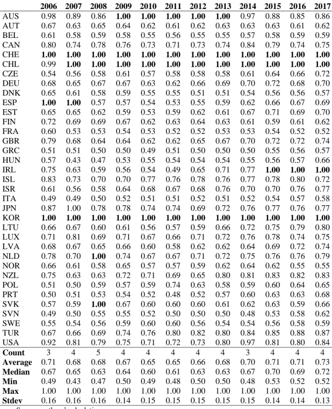
We performed the DEA considering three models: baseline model (Model 0), which includes only one input (PE as percentage of GDP) and one output (PSP); Model 1 uses one input, governments’ normalized total spending (PE) and two outputs, the opportunity PSP and the “Musgravian” PSP scores; and Model 2 assumes two inputs, governments’ normalized spending on opportunity and on “Musgravian” indicators and one output, total PSP scores.

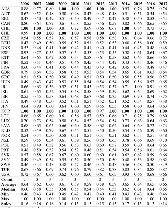
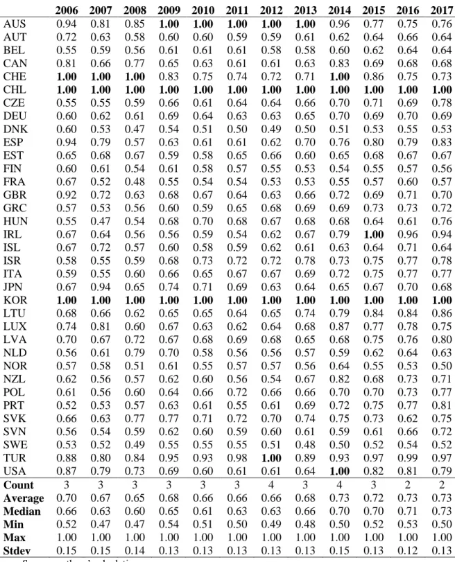
The detailed input efficient scores are illustrated on Tables 6, 7 and 8. In this analysis, we exclude Mexico because the country is efficient by default,9 and data heterogeneity is quite important for the country sample analysis. In addition, Table 9 provides a summary of the DEA results for the three models using an input-oriented assessment. The purpose of an input-oriented assessment is to study by how much input quantities can be proportionally reduced without changing the output quantities produced. The average efficiency score throughout the period is around 0.6 for the 1 input and 1 output model (Model 0) and around 0.7 in the alternative models (Models 1 and 2). Interestingly, the average input efficiency scores have increased slightly between 2006 and 2017. Nevertheless, these results imply that some possible efficiency gains could be achieved with around less 30% government spending, on average, without changing the PSP outputs. [insert Table 6] [insert Table 7] [insert Table 8] [insert Table 9]

(13)

11

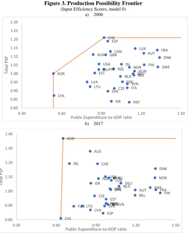
Figure 3. Production Possibility Frontier

(Input Efficiency Scores, model 0) a) 2006

b) 2017

Source: authors’ calculations.

Note: Figure 3 plots the production possibility frontiers for Model 0 for the years 2006 and 2017. In the vertical axis we have the total Public Sector Performance (PSP) composite indicator AUS – Australia; AUT- Austria; BEL – Belgium; CAN – Canada; CHE – Switzerland; CHL – Chile; CZE – Czech Republic; DEU – Germany; DNK – Denmark; ESP – Spain; EST – Estonia; FIN – Finland; FRA – France; GBR – United kingdom; GRC – Greece; HUN – Hungary; IRL – Ireland; ISL – Iceland; ISR – Israel; ITA – Italy; JPN – Japan; KOR – South Korea; LTU – Lithuania; LUX – Luxembourg; LVA – Latvia; MEX – Mexico; NLD – Netherlands; NOR – Norway; NZL – New Zealand; POL – Poland; PRT – Portugal; SVK – Slovak Republic; SVN – Slovenia; SWE – Sweden; TUR – Turkey; USA – United States of America.

AUS AUT BEL CAN CHE CHL CZE DEU DNK ESP EST FIN FRA GBR GRC HUN IRL ISL ISR ITA JPN KOR LTU LUX LVA NLD NOR NZL PRT SVK SVN SWE USA 0.80 0.85 0.90 0.95 1.00 1.05 1.10 1.15 1.20 1.25 1.30 0.30 0.60 0.90 1.20 1.50 To ta l PSP

Public Expenditure-to-GDP ratio

AUS AUT BEL CAN CHE CHL CZE DEU DNK ESP EST FIN FRA GBR HUN IRL ISL ISR JPN KOR LTU LUX LVA NLD NOR NZL POL_PRT SVK SVN SWE TUR USA 0.80 0.90 1.00 1.10 1.20 1.30 1.40 0.30 0.60 0.90 1.20 1.50 Tot al PSP

(14)

12

Figure 3 illustrates the production possibility frontier for the baseline model (Model 0), for 2006 (first year of our sample) and for 2017 (last year of our sample), pinpointing notably the countries that define the frontier: Switzerland and Korea in 2006, and Chile and Korea in 2017. For all the other countries inside the frontier, theoretically there would be room for improvement regarding efficiency gains.

Tables 10, 11 and 12 present the efficiency scores considering the output perspective. By computing output-oriented measures, one can assess how much output quantities can be proportionally increased without changing the input quantities used. Note that since Greece’s PSP score is negative in 2012 and 2013, we cannot compute its efficiency score for Model 0 and 1.

[insert Table 10] [insert Table 11] [insert Table 12]

Finally, Table 13 provides a summary of the DEA results for the three models using output oriented models. The average output efficiency score is approximately 1.50 for Models 0 and 1 and 1.16 for Model 3 suggesting that outputs could be increased by approximately 50% or 16%. The output efficiency scores for Models 0 and 1 where somewhat higher and seemed to have peaked in the period 2011-2013, and then they decreased.

[insert Table 13]

6. Conclusion

In this study, we provided a review of the literature dealing with overall public sector performance and efficiency. Moreover, we outlined a methodology to assess public sector efficiency and we have created a novel and large cross-country panel dataset of government indicators and public sector efficiency scores, covering all 36 OECD countries over the 2006-2017 time period. In practice, we used economic and sociodemographic indicators to construct performance composite indicators, and then we computed input and output oriented efficiency scores solving the several DEA problems.

(15)

13

The average input efficiency score in the period 2006-2017 was found to be around 0.6-0.7 implying that some efficiency gains could be achieved with around less 30-40% government spending, on average without changing the overall level of performance. The average output efficiency score was found to be between 1.16 and 1.50 suggesting that outputs could be increased by approximately 16-50%.

With this study, we fulfilled a gap in the literature, by providing a cross-country data set of public sector performance indicators and efficiency scores, which can be useful for further research by other authors.

References

Adam, A., Delis, M., Kammas, P. (2011). “Public sector efficiency: leveling the playing field between OECD countries”, Public Choice, 146, 163–183.

Afonso, A., Furceri, D. (2010). “Government Size, Composition, Volatility and Economic Growth”, European Journal of Political Economy, 26 (4), 517-532.

Afonso, A., Jalles, J. (2016). “Economic Performance, Government Size, and Institutional Quality”, Empirica, 43 (1), 83-109.

Afonso, A., Kazemi, M. (2017). “Assessing Public Spending Efficiency in 20 OECD Countries”, in Inequality and Finance in Macrodynamics (Dynamic Modeling and Econometrics in Economics and Finance), Bettina Bökemeier and Alfred Greiner (Editors). Springer.

Afonso, A., Romero, A., Monsalve, E. (2013). “Public Sector Efficiency: Evidence for Latin America Public”. Inter-American Development Bank, 80478, Inter-American Development Bank.

Afonso, A., St. Aubyn (2006). “Cross-country Efficiency of Secondary Education Provision: a Semi-parametric Analysis with Non-discretionary Inputs,” Economic Modelling, 23 (3), 476-491.

Afonso, A., St. Aubyn, M. (2013). “Public and Private Inputs in Aggregate Production and Growth: A Cross-country Efficiency Approach”, Applied Economics, 45 (32), 4451-4466. Afonso, A.; Schuknecht, L., Tanzi, V. (2005). “Public Sector Efficiency: An International

Comparison,” Public Choice, 123 (3-4), 321-347.

Afonso, A.; Schuknecht, L., Tanzi, V. (2010). “Public Sector Efficiency: Evidence for New EU Member States and Emerging Markets”, Applied Economics, 42 (17), 2147-2164.

(16)

14

Afonso, A., Venâncio, A. (2019). “Local Territorial Reform and Regional Spending Efficiency”, Local Government Studies, forthcoming.

Amaglobeli, D., Crispolti, V., Dabla-Norris, E., Karnane, P., Misch. F. (2018). “Tax Policy Measures in Advanced and Emerging Economies: A Novel Database”, IMF WP 18/110. Antonelli, M., de Bonis, V. (2019). “The efficiency of social public expenditure in European

countries: a two-stage analysis”, Applied Economics, 51 (1), 47-60.

Armey, D. (1995). “The freedom revolution: the new republican house majority leader tells why big governments failed, why freedom works and how we will rebuild America”, Washington, DC, Regnery Publishing Inc.

Auerbach, A., Gorodnichenko. Y. (2013). “Output Spillovers from Fiscal Policy”, American Economic Review, 103 (3), 141-46.

Chan, S.-G., Ramly, Z., Karim, M. (2017). “Government Spending Efficiency on Economic Growth: Roles of Value-added Tax”, Global Economic Review, 46 (2), 162-188.

Dutu, R., Sicari, P. (2016). “Public Spending Efficiency in the OECD: Benchmarking Health Care, Education and General Administration”, OECD Economics Department Working Papers 1278.

EC (2007). The EU economy: 2007 review, Moving Europe's productivity frontier. November, European Commission.

Hauner, D., Kyobe, A. (2010). “Determinants of Government Efficiency”, World Development, 38 (11), 1527–1542.

Henderson, D., Russel, R. (2005). “Human capital and convergence: a production-frontier approach”, International Economic Review, 46 (4), 1167-1205.

Herrera, S., Ouedraogo, A. (2018). Efficiency of Public Spending in Education, Health, and Infrastructure: An International Benchmarking Exercise, World Bank Policy Research Working Paper 8586.

Jorda, O. (2005). “Estimation and inference of impulse responses by local projections”. American Economic Review, 95(1), 161–182.

Krüger, J. (2003). “The global trends of total factor productivity: evidence from the nonparametric Malmquist index approach”, Oxford Economic Papers, 55, 265-286.

(17)

15

Kumar, S., Russell, R. (2002). “Technological Change, Technological Catch-up, and Capital Deepening: Relative Contributions to Growth and Convergence”, American Economic Review, 92 (3), 527-548.

Labonte, M. (2010), “The Size and Role of Government: Economic Issues”, Congressional Research Service 7-5700, RL32162.

Lamartina, S., Zaghini, A. (2011), “Increasing Public Expenditure: Wagner's Law in OECD Countries”, German Economic Review, 12(2), 149-164.

Montes, G., Bastos, J., de Oliveira, A. (2019). “Fiscal transparency, government effectiveness and government spending efficiency: Some international evidence based on panel data approach”, Economic Modelling, 79, 211-225.

Mohanty, R., Bhanumurthy, N. (2018). “Assessing Public Expenditure Efficiency at Indian States”, National Institute of Public Finance and Policy, New Delhi, NIPFP Working Paper 225.

Pesaran, M., (2006). “Estimation and inference in large heterogeneous panels with a multifactor error structure”, Econometrica, 74 (4), 967-1012.

Pesaran, M., Shin, Y., Smith, R. (1999). “Pooled mean group estimation of dynamic heterogeneous panels”, Journal of American Statistical Association, 94, 31-54.

Qazizada, W, Stockhammer, E. (2015). “Government spending multipliers in contraction and expansion”, International Review of Applied Economics, 29 (2), 238-258.

Simar, L., Wilson, P., (2007). “Estimation and Inference in Two-Stage, Semi-Parametric Models of Production Processes”. Journal of Econometrics, 136 (1), 31-64.

(18)

16

Table 1: Overall public sector efficiency

Authors Sample Methods Results

Afonso,

Schuknecht, Tanzi (2005)

23 OECD countries FDH The average input efficiency score of the 15 EU countries is 0.73 (around 27% could be reduced).

Adam, Delis, Kammas (2011) 19 OECD countries,1980-2000 Stochastic DEA

Countries with right-wing and strong governments, high voter participation rates and decentralized fiscal systems, are expected to have higher PSE.

Afonso, Romero, Monsalve (2013)

Latin American and Caribbean countries, 2001-2010

DEA Output efficiency scores higher than input efficiency scores. PSE is inversely correlated with the size of the government, while the efficiency frontier is defined by Chile, Guatemala, and Peru.

Dutu, Sicari (2016) 35 OECD countries, 2012 DEA Wide dispersion in efficiency measures across OECD, health care, education, general administration.

Chan et al. (2017) 115 countries Panel GMM VAT system enhances the effect of efficient government spending on the economic growth.

Herrera, Ouedrago (2018)

175 countries for 2006-2016 on education, health, infrastructure

FDH, DEA The efficiency of capital spending is correlated with regulatory quality and perception of corruption.

Mohanty, Bhanumurthy (2018)

27 Indian States, 2000-2015 DEA Higher efficiency on education than on health and overall social spending. Governance and growth affects the efficiency.

Montes, Bastos, Oliveira (2019)

68 developing and 14 developed countries, 2006– 2014

Panel, GMM Fiscal transparency affects government spending efficiency.

Antonelli, de Bonis (2019)

22 EU countries, 2013 Median voter model

More efficient have higher education and GDP levels, smaller population size, lower degree of selectivity of their welfare systems and a lower corruption level.

(19)

17

Table 2: DEA Output Components

Sub Index Variable Source Series

Opportunity Indicators

Administration Corruption Transparency International’s

Corruption Perceptions Index (CPI) (2006- 2017)

Corruption on a scale from 10 (Perceived to have low levels of corruption) to 0 (highly corrupt), 2006-2011; Corruption on a scale from 100 (Perceived to have low levels of corruption) to 0 (highly corrupt), 2012-2017.

Red Tape World Economic Forum: The Global competitiveness Report (2006-2017)

Burden of government regulation on a scale from 7 (not burdensome at all) to 1 (extremely burdensome). Judicial

Independence

World Economic Forum: The Global competitiveness Report (2006-2017)

Judicial independence on a scale from 7 (entirely independent) to 1 (heavily influenced).

Property Rights World Economic Forum: The Global competitiveness Report (2006-2017)

Property rights on a scale from 7 (very strong) to 1 (very weak).

Shadow Economy Schneider (2016) (2006-2016)10 _{Shadow economy measured as percentage of official GDP.}

Reciprocal value 1/x.

Education Secondary School

Enrolment

World Bank, World Development Indicators (2006-2017)

Ratio of total enrolment in secondary education. Quality of

Educational System

Quality of educational system on a scale from 7 (very well) to 1 (not well at all).

PISA scores PISA Report (2003, 2006, 2009, 2012, 2015)

Simple average of mathematics, reading and science scores for the years 2015, 2012, 2009; Simple average of mathematics and reading for the year 2003. For the missing years, we assumed that the scores were the same as in the previous years.

Health Infant Survival

Rate

World Bank, World Development Indicators (2006-2017)

Infant survival rate = (1000-IMR)/1000. IMR is the infant mortality rate measured per 1000 lives birth in a given year. Life Expectancy World Bank, World Development

Indicators (2006-2017)

Life expectancy at birth, measured in years. CVD, cancer,

diabetes or CRD Survival Rate

World Health Organization, Global Health Observatory Data

Repository (2000, 2005, 2010, 2015, 2016)

CVD, cancer and diabetes survival rate =100-M. M is the mortality rate between the ages 30 and 70. For the missing years, we assumed that the scores were the same as in the previous years.

Public Infrastructure

Infrastructure Quality

Infrastructure quality on a scale from 7 (extensive and efficient) to 1 (extremely underdeveloped)

Standard Musgravian Indicators

Distribution Gini Index Eurostat, OECD (2006-2016)11 _{Gini index on a scale from 1(perfect inequality) to 0 (perfect}

equality). Transformed to 1-Gini.

Stabilization Coefficient of

Variation of Growth

IMF World Economic Outlook (WEO database) (2006-2017)

Coefficient of variation=standard deviation/mean of GDP growth based on 5 year data. GDP constant prices (percent change). Reciprocal value 1/x.

Standard Deviation of Inflation

Standard deviation of inflation based on 5-year consumer prices (percent change) data. Reciprocal value 1/x.

Economic Performance

GDP per Capita IMF World Economic Outlook (WEO database) (2006-2017)

GDP per capita based on PPP, current international dollar. GDP Growth IMF World Economic Outlook

(WEO database) (2006-2017)

GDP constant prices (percent change). Unemployment IMF World Economic Outlook

(WEO database) (2006-2017)

Unemployment rate, as a percentage of total labor force. Reciprocal value 1/x.

10_{For Chile, Iceland, Israel, South Korea and Mexico, we use the data available in Medina and Schneider (2017).} 11_{For Switzerland, we were only able to collect data for the period between 2009 and 2016.}

(20)

18

Table 3: Input Components

Sub Index Variable Source Series

Opportunity Indicators

Administration

Government Consumption

General government final consumption expenditure (% of GDP) at current prices

Education

Education Expenditure

UNESCO Institute for Statistics (2005-2016)12

Expenditure on education (% of GDP)

Health

Health

Expenditure OECD database (2005-2016)

Expenditure on health (% of GDP) Public Infrastructure Public Investment

European Commission, AMECO (2005-2016)13

General government gross fixed capital formation (% of GDP) at current prices Standard Musgravian Indicators Distribution Social Protection

Expenditure OECD database (2005-2016)14

Aggregation of the social transfers (% of GDP) Stabilization/

Economic Performance

Government Total

Expenditure OECD database (2005-2016)15

Expenditure total expenditure (% of GDP)

12_{From IMF World Economic Outlook (WEO database), we retrieved data for Greece for the period between 2006} and 2012 and for the USA for the period 2005 and 2007.

13_{We were not able to collect data on the following countries: Australia, Canada, Mexico, New Zealand, Chile, Israel} and South Korea.

14_{From IMF World Economic Outlook (WEO database), we retrieved data for New Zealand for the period 2005 and} 2012. For Turkey, we retrieve data from European Commission, AMECO database. For Chile and Iceland, we were only able to collect data for the period between 2013 and 2016. For Turkey, we were only able to get data for the period between 2009 and 2015. We were not able to collect data for Canada.

15_{From IMF World Economic Outlook (WEO database), we retrieved data for Canada for the period between 2005} and 2012 and for New Zealand for the period 2009 and 2012. For Turkey, we retrieve data from European Commission, AMECO database. We were not able to collect data for Mexico. For Chile and Iceland, we were only able to collect data for the period between 2013 and 2016. For New Zealand, we were only able to collect data for the period between 2009 and 2016. For Japan, we were only able to collect data for the period between 2005 and 2016.

(21)

19

Table 4: PSP Standardized Indicator

2006 2007 2008 2009 2010 2011 2012 2013 2014 2015 2016 2017 AUS 1.11 1.09 1.27 1.35 1.45 1.53 2.16 1.94 1.22 1.19 1.17 1.28 AUT 1.12 1.09 1.21 1.09 1.09 1.10 1.07 0.97 1.03 1.00 1.02 1.01 BEL 0.99 1.00 1.01 0.98 1.02 1.02 0.98 0.96 0.96 0.96 0.98 0.97 CAN 1.13 1.08 1.31 1.05 1.10 1.10 1.19 1.17 1.24 1.08 1.13 1.09 CHE 1.21 1.23 1.35 1.20 1.25 1.25 1.28 1.34 1.33 1.29 1.27 1.19 CHL 0.87 0.87 1.10 0.89 1.03 1.07 1.43 1.30 0.94 0.92 0.85 0.81 CZE 0.91 0.94 1.09 0.94 0.92 0.90 0.76 0.77 0.91 0.96 0.91 0.97 DEU 1.00 0.98 1.09 1.03 1.08 1.08 1.05 1.02 1.09 1.04 1.06 1.06 DNK 1.09 1.07 0.99 1.08 1.04 1.00 0.96 0.96 1.06 1.05 1.05 1.16 ESP 1.19 1.15 1.03 0.89 0.83 0.76 0.41 0.37 0.78 0.83 0.85 0.85 EST 1.00 0.99 0.40 0.95 0.79 0.91 1.02 0.86 0.94 0.89 0.93 0.94 FIN 1.05 1.07 1.05 1.07 1.05 1.04 0.84 0.89 0.95 0.91 0.97 0.99 FRA 1.14 1.06 1.01 0.99 1.00 1.01 0.96 0.97 1.00 0.97 0.99 1.01 GBR 1.11 1.08 0.89 1.02 1.00 0.96 1.02 1.02 1.11 1.07 1.07 1.02 GRC 0.95 0.95 0.82 0.87 0.61 0.42 -0.22 -0.12 0.62 0.64 0.67 0.71 HUN 1.01 0.76 0.82 0.83 0.75 0.75 0.60 0.76 0.86 0.83 0.80 0.91 IRL 1.02 1.02 0.65 0.91 0.87 0.91 0.80 0.93 1.11 1.43 1.06 1.19 ISL 1.05 1.12 1.14 1.05 0.84 0.94 0.91 1.01 0.99 1.11 1.18 1.09 ISR 0.84 0.89 1.09 1.01 1.21 1.28 1.49 1.55 1.03 0.98 1.07 1.06 ITA 0.92 0.89 0.73 0.84 0.82 0.77 0.44 0.55 0.73 0.73 0.73 0.80 JPN 1.03 1.20 0.89 0.99 1.04 0.94 1.04 1.10 0.99 1.03 1.04 1.01 KOR 1.00 1.05 1.23 1.15 1.32 1.29 1.49 1.43 1.06 1.18 1.29 1.37 LTU 0.92 0.95 0.97 0.90 0.74 0.85 0.96 0.87 0.92 0.89 0.94 0.90 LUX 1.15 1.16 0.98 1.12 1.19 1.12 0.99 1.21 1.19 1.08 1.09 1.08 LVA 0.95 0.96 0.44 0.87 0.57 0.78 0.87 0.76 0.79 0.88 0.92 0.87 MEX 0.80 0.79 0.87 0.85 0.93 0.90 1.14 0.93 1.08 1.00 0.94 0.81 NLD 0.98 1.09 1.35 1.23 1.17 1.13 0.94 0.90 0.99 1.01 1.00 1.03 NOR 1.04 1.06 1.07 1.13 1.09 1.09 1.30 1.19 1.16 1.17 1.07 1.09 NZL 1.03 1.03 0.92 1.09 1.14 1.13 1.35 1.55 1.20 1.11 1.24 1.09 POL 0.80 0.82 1.12 1.04 1.21 1.38 1.63 1.31 0.90 0.89 0.90 0.91 PRT 0.83 0.86 0.97 0.86 0.87 0.74 0.35 0.53 0.78 0.80 0.82 0.91 SVK 0.90 0.89 1.23 0.92 0.96 0.89 0.95 0.84 0.87 0.91 0.90 0.90 SVN 0.94 0.94 1.19 0.99 0.89 0.84 0.54 0.67 0.88 0.84 0.86 0.91 SWE 1.04 1.05 0.92 1.05 1.18 1.10 0.96 1.07 1.05 1.17 1.14 1.03 TUR 0.80 0.76 0.79 0.81 0.98 1.06 1.22 1.31 0.99 0.97 0.93 0.89 USA 1.06 1.06 1.01 0.96 0.98 0.95 1.11 1.10 1.25 1.18 1.15 1.10 Average 1 1 1 1 1 1 1 1 1 1 1 1 Median 1.01 1.02 1.01 0.99 1.01 1.01 0.98 0.97 0.99 0.99 0.99 1.01 Min 0.80 0.76 0.40 0.81 0.57 0.42 -0.22 -0.12 0.62 0.64 0.67 0.71 Max 1.21 1.23 1.35 1.35 1.45 1.53 2.16 1.94 1.33 1.43 1.29 1.37 Stdev 0.11 0.12 0.22 0.12 0.19 0.21 0.41 0.36 0.16 0.16 0.14 0.14

(22)

20

Table 5: PE Standardized Indicator

2006 2007 2008 2009 2010 2011 2012 2013 2014 2015 2016 2017 AUS 0.84 0.84 0.84 0.86 0.80 0.80 0.81 0.81 0.82 0.84 0.85 0.86 AUT 1.22 1.21 1.21 1.19 1.17 1.17 1.16 1.16 1.18 1.19 1.18 1.20 BEL 1.15 1.12 1.13 1.14 1.13 1.12 1.16 1.19 1.20 1.20 1.19 1.19 CAN 0.97 0.98 1.00 0.96 0.98 1.00 0.99 0.98 0.96 0.94 0.98 1.00 CHE 0.92 0.88 0.85 0.83 0.81 0.82 0.84 0.86 0.87 0.87 0.88 0.91 CHL 0.54 0.53 0.55 0.57 0.56 0.55 0.55 0.56 0.58 0.60 0.63 0.63 CZE 1.00 0.99 0.96 0.95 0.97 0.95 0.95 0.96 0.94 0.94 0.96 0.89 DEU 1.14 1.12 1.09 1.06 1.09 1.08 1.06 1.06 1.06 1.06 1.06 1.09 DNK 1.34 1.32 1.33 1.29 1.32 1.35 1.37 1.37 1.37 1.35 1.34 1.35 ESP 0.95 0.96 0.99 1.00 1.03 1.04 1.04 1.02 0.99 0.98 0.98 0.95 EST 0.85 0.86 0.89 0.99 1.05 0.94 0.90 0.96 0.93 0.92 0.96 0.98 FIN 1.22 1.20 1.18 1.17 1.22 1.22 1.25 1.32 1.35 1.37 1.36 1.38 FRA 1.32 1.32 1.33 1.30 1.28 1.29 1.30 1.32 1.33 1.33 1.31 1.35 GBR 0.93 0.97 0.98 1.01 1.01 1.03 1.03 1.03 1.02 1.01 1.00 1.01 GRC 1.06 1.10 1.10 1.15 1.14 1.08 1.10 1.12 1.15 1.09 1.12 1.11 HUN 1.15 1.21 1.16 1.08 1.02 1.02 1.02 1.02 1.04 1.07 1.11 0.98 IRL 0.88 0.90 0.98 1.10 1.08 1.23 1.04 0.98 0.93 0.87 0.70 0.70 ISL 1.05 1.07 1.08 1.09 0.97 0.95 0.93 0.95 0.95 0.97 0.93 1.04 ISR 0.97 0.97 0.95 0.92 0.85 0.85 0.85 0.87 0.87 0.86 0.86 0.86 ITA 1.10 1.11 1.10 1.10 1.09 1.07 1.07 1.09 1.10 1.10 1.09 1.09 JPN 0.92 0.91 0.92 0.91 0.93 0.94 1.00 1.01 1.02 1.01 0.99 1.01 KOR 0.54 0.57 0.58 0.60 0.59 0.57 0.59 0.60 0.61 0.63 0.64 0.65 LTU 0.81 0.84 0.91 0.94 1.00 0.95 0.94 0.84 0.81 0.80 0.80 0.80 LUX 1.15 1.04 1.01 1.03 1.06 1.06 1.02 1.03 1.00 0.99 0.99 1.02 LVA 0.79 0.85 0.85 0.87 0.93 0.94 0.90 0.90 0.89 0.86 0.88 0.86 MEX 0.42 0.42 0.44 0.45 0.43 0.43 0.44 0.44 0.43 0.44 0.44 0.44 NLD 1.04 1.08 1.07 1.06 1.07 1.09 1.10 1.11 1.10 1.09 1.07 1.07 NOR 1.11 1.07 1.11 1.05 1.11 1.09 1.09 1.10 1.14 1.19 1.26 1.34 NZL 0.99 1.02 1.01 0.98 0.96 1.00 1.11 1.00 0.95 0.94 0.93 0.92 POL 1.06 1.08 1.06 1.06 0.99 1.04 1.03 0.99 0.98 1.00 0.98 0.98 PRT 1.11 1.07 1.06 1.05 1.08 1.14 1.09 1.04 1.06 1.06 1.04 0.99 SVK 0.95 0.92 0.89 0.86 0.93 0.92 0.92 0.91 0.93 0.96 1.07 0.96 SVN 1.10 1.10 1.06 1.06 1.07 1.10 1.12 1.11 1.20 1.13 1.09 1.03 SWE 1.33 1.30 1.27 1.24 1.22 1.19 1.24 1.30 1.31 1.30 1.27 1.31 TUR 0.80 0.80 0.79 0.77 0.73 0.69 0.68 0.72 0.72 0.71 0.72 0.73 USA 0.88 0.88 0.91 0.94 0.93 0.91 0.91 0.88 0.85 0.94 0.95 0.97 Average 1 1 1 1 1 1 1 1 1 1 1 1 Median 0.99 1.00 1.00 1.02 1.01 1.03 1.03 1.00 0.99 0.98 0.99 0.98 Min 0.42 0.42 0.44 0.45 0.43 0.43 0.44 0.44 0.43 0.44 0.44 0.44 Max 1.34 1.32 1.33 1.30 1.32 1.35 1.37 1.37 1.37 1.37 1.36 1.38 Stdev 0.21 0.20 0.20 0.19 0.19 0.20 0.20 0.20 0.21 0.21 0.21 0.21

(23)

21

Table 6: Input-oriented DEA VRS Efficiency Scores Model 0

2006 2007 2008 2009 2010 2011 2012 2013 2014 2015 2016 2017 AUS 0.88 0.77 0.80 1.00 1.00 1.00 1.00 1.00 0.93 0.76 0.75 0.76 AUT 0.62 0.52 0.48 0.50 0.48 0.47 0.48 0.48 0.51 0.51 0.54 0.54 BEL 0.47 0.50 0.49 0.51 0.50 0.49 0.47 0.47 0.48 0.50 0.53 0.54 CAN 0.80 0.64 0.77 0.61 0.58 0.55 0.56 0.57 0.82 0.66 0.65 0.65 CHE 1.00 1.00 1.00 0.81 0.72 0.69 0.66 0.67 1.00 0.84 0.73 0.71 CHL 0.99 1.00 1.00 1.00 1.00 1.00 1.00 1.00 1.00 1.00 1.00 1.00 CZE 0.54 0.55 0.57 0.61 0.57 0.58 0.58 0.58 0.61 0.64 0.66 0.72 DEU 0.47 0.49 0.50 0.55 0.52 0.51 0.52 0.53 0.60 0.58 0.60 0.59 DNK 0.53 0.46 0.41 0.46 0.42 0.41 0.40 0.41 0.44 0.45 0.48 0.48 ESP 0.93 0.77 0.55 0.57 0.54 0.53 0.53 0.55 0.58 0.61 0.64 0.67 EST 0.64 0.65 0.62 0.58 0.53 0.58 0.61 0.58 0.62 0.65 0.66 0.65 FIN 0.52 0.51 0.46 0.51 0.46 0.45 0.44 0.42 0.43 0.43 0.46 0.46 FRA 0.60 0.44 0.41 0.45 0.44 0.43 0.43 0.42 0.45 0.45 0.48 0.47 GBR 0.79 0.64 0.56 0.58 0.55 0.53 0.54 0.54 0.65 0.61 0.63 0.64 GRC 0.51 0.50 0.50 0.50 0.49 0.51 0.50 0.50 0.50 0.55 0.56 0.57 HUN 0.49 0.43 0.47 0.53 0.55 0.54 0.54 0.54 0.55 0.56 0.57 0.65 IRL 0.66 0.63 0.56 0.52 0.51 0.45 0.53 0.57 0.71 1.00 0.91 0.92 ISL 0.61 0.65 0.52 0.54 0.58 0.58 0.59 0.59 0.62 0.64 0.69 0.62 ISR 0.55 0.55 0.58 0.64 0.68 0.67 0.68 0.75 0.69 0.70 0.74 0.75 ITA 0.49 0.48 0.50 0.52 0.51 0.51 0.52 0.51 0.52 0.54 0.57 0.58 JPN 0.64 0.90 0.60 0.64 0.60 0.59 0.55 0.55 0.58 0.60 0.64 0.63 KOR 1.00 1.00 1.00 1.00 1.00 1.00 0.97 1.00 1.00 1.00 1.00 1.00 LTU 0.66 0.65 0.60 0.61 0.56 0.57 0.59 0.66 0.71 0.75 0.79 0.80 LUX 0.70 0.73 0.54 0.58 0.54 0.52 0.54 0.54 0.73 0.63 0.64 0.63 LVA 0.68 0.65 0.65 0.66 0.60 0.58 0.62 0.62 0.64 0.69 0.72 0.74 NLD 0.52 0.59 0.79 0.67 0.54 0.51 0.50 0.50 0.54 0.56 0.59 0.60 NOR 0.54 0.54 0.50 0.58 0.51 0.51 0.51 0.51 0.62 0.53 0.51 0.48 NZL 0.59 0.55 0.54 0.61 0.59 0.56 0.50 0.65 0.78 0.66 0.69 0.70 POL 0.51 0.49 0.52 0.56 0.58 0.63 0.60 0.57 0.59 0.60 0.64 0.65 PRT 0.48 0.50 0.52 0.54 0.52 0.48 0.51 0.54 0.54 0.56 0.61 0.64 SVK 0.57 0.58 0.67 0.67 0.60 0.60 0.60 0.61 0.62 0.62 0.59 0.66 SVN 0.49 0.49 0.54 0.55 0.52 0.50 0.50 0.50 0.48 0.53 0.58 0.62 SWE 0.46 0.44 0.43 0.48 0.47 0.46 0.45 0.43 0.46 0.48 0.50 0.49 TUR 0.67 0.66 0.69 0.74 0.76 0.79 0.82 0.78 0.83 0.84 0.88 0.87 USA 0.72 0.67 0.60 0.62 0.60 0.60 0.61 0.63 0.93 0.66 0.68 0.66 Count 2 3 3 3 3 3 2 3 3 3 2 2 Average 0.64 0.62 0.60 0.61 0.59 0.58 0.58 0.59 0.65 0.64 0.65 0.66 Median 0.60 0.58 0.55 0.58 0.55 0.54 0.54 0.55 0.62 0.61 0.64 0.65 Min 0.46 0.43 0.41 0.45 0.42 0.41 0.40 0.41 0.43 0.43 0.46 0.46 Max 1.00 1.00 1.00 1.00 1.00 1.00 1.00 1.00 1.00 1.00 1.00 1.00 Stdev 0.16 0.16 0.16 0.14 0.15 0.15 0.15 0.15 0.17 0.15 0.13 0.14

(24)

22

2006 2007 2008 2009 2010 2011 2012 2013 2014 2015 2016 2017 AUS 0.94 0.81 0.85 1.00 1.00 1.00 1.00 1.00 0.96 0.77 0.75 0.76 AUT 0.72 0.63 0.58 0.60 0.60 0.59 0.59 0.61 0.62 0.64 0.66 0.64 BEL 0.55 0.59 0.56 0.61 0.61 0.61 0.58 0.58 0.60 0.62 0.64 0.64 CAN 0.81 0.66 0.77 0.65 0.63 0.61 0.61 0.63 0.83 0.69 0.68 0.68 CHE 1.00 1.00 1.00 0.83 0.75 0.74 0.72 0.71 1.00 0.86 0.75 0.73 CHL 1.00 1.00 1.00 1.00 1.00 1.00 1.00 1.00 1.00 1.00 1.00 1.00 CZE 0.55 0.55 0.59 0.66 0.61 0.64 0.64 0.66 0.70 0.71 0.69 0.78 DEU 0.60 0.62 0.61 0.69 0.64 0.63 0.63 0.65 0.70 0.69 0.70 0.69 DNK 0.60 0.53 0.47 0.54 0.51 0.50 0.49 0.50 0.51 0.53 0.55 0.53 ESP 0.94 0.79 0.57 0.63 0.61 0.61 0.62 0.70 0.76 0.80 0.79 0.83 EST 0.65 0.68 0.67 0.59 0.58 0.65 0.66 0.60 0.65 0.68 0.67 0.67 FIN 0.60 0.61 0.54 0.61 0.58 0.57 0.55 0.53 0.54 0.55 0.57 0.56 FRA 0.67 0.52 0.48 0.55 0.54 0.54 0.53 0.53 0.55 0.57 0.60 0.57 GBR 0.92 0.72 0.63 0.68 0.67 0.64 0.63 0.66 0.72 0.69 0.71 0.70 GRC 0.57 0.53 0.56 0.60 0.59 0.65 0.68 0.69 0.69 0.73 0.73 0.72 HUN 0.55 0.47 0.54 0.68 0.70 0.68 0.67 0.68 0.68 0.64 0.61 0.76 IRL 0.67 0.64 0.56 0.56 0.59 0.54 0.62 0.67 0.79 1.00 0.96 0.94 ISL 0.67 0.72 0.57 0.60 0.58 0.59 0.62 0.61 0.63 0.64 0.71 0.64 ISR 0.58 0.55 0.59 0.68 0.73 0.72 0.72 0.78 0.73 0.75 0.77 0.78 ITA 0.59 0.55 0.60 0.66 0.65 0.67 0.67 0.69 0.72 0.75 0.77 0.77 JPN 0.67 0.94 0.65 0.74 0.71 0.69 0.63 0.64 0.65 0.67 0.70 0.68 KOR 1.00 1.00 1.00 1.00 1.00 1.00 1.00 1.00 1.00 1.00 1.00 1.00 LTU 0.68 0.66 0.62 0.65 0.65 0.64 0.65 0.74 0.79 0.84 0.84 0.86 LUX 0.74 0.81 0.60 0.67 0.63 0.62 0.64 0.68 0.87 0.77 0.78 0.75 LVA 0.70 0.67 0.72 0.67 0.68 0.69 0.68 0.65 0.68 0.75 0.76 0.80 NLD 0.56 0.61 0.79 0.70 0.58 0.56 0.56 0.57 0.59 0.62 0.64 0.63 NOR 0.57 0.58 0.51 0.61 0.55 0.57 0.57 0.56 0.64 0.55 0.53 0.50 NZL 0.62 0.56 0.57 0.62 0.60 0.56 0.54 0.67 0.82 0.68 0.73 0.71 POL 0.61 0.56 0.60 0.64 0.66 0.72 0.66 0.66 0.70 0.70 0.73 0.77 PRT 0.52 0.53 0.57 0.63 0.61 0.55 0.61 0.69 0.72 0.75 0.77 0.81 SVK 0.66 0.63 0.77 0.77 0.71 0.72 0.70 0.74 0.75 0.73 0.62 0.75 SVN 0.56 0.54 0.59 0.62 0.60 0.59 0.60 0.61 0.59 0.61 0.66 0.72 SWE 0.53 0.52 0.49 0.55 0.55 0.55 0.51 0.48 0.50 0.52 0.54 0.52 TUR 0.88 0.80 0.84 0.95 0.93 0.98 1.00 0.89 0.93 0.97 0.99 0.97 USA 0.87 0.79 0.73 0.69 0.60 0.61 0.61 0.64 1.00 0.82 0.81 0.79 Count 3 3 3 3 3 3 4 3 4 3 2 2 Average 0.70 0.67 0.65 0.68 0.66 0.66 0.66 0.68 0.73 0.72 0.73 0.73 Median 0.66 0.63 0.60 0.65 0.61 0.63 0.63 0.66 0.70 0.70 0.71 0.73 Min 0.52 0.47 0.47 0.54 0.51 0.50 0.49 0.48 0.50 0.52 0.53 0.50 Max 1.00 1.00 1.00 1.00 1.00 1.00 1.00 1.00 1.00 1.00 1.00 1.00 Stdev 0.15 0.15 0.14 0.13 0.13 0.13 0.13 0.13 0.15 0.13 0.12 0.13

(25)

23

2006 2007 2008 2009 2010 2011 2012 2013 2014 2015 2016 2017 AUS 0.98 0.89 0.86 1.00 1.00 1.00 1.00 1.00 0.97 0.88 0.85 0.86 AUT 0.67 0.63 0.65 0.64 0.62 0.61 0.62 0.63 0.63 0.63 0.61 0.62 BEL 0.61 0.58 0.59 0.58 0.55 0.56 0.55 0.55 0.57 0.58 0.59 0.59 CAN 0.80 0.74 0.78 0.76 0.73 0.71 0.73 0.74 0.84 0.79 0.74 0.75 CHE 1.00 1.00 1.00 1.00 1.00 1.00 1.00 1.00 1.00 1.00 1.00 1.00 CHL 0.99 1.00 1.00 1.00 1.00 1.00 1.00 1.00 1.00 1.00 1.00 1.00 CZE 0.54 0.56 0.58 0.61 0.57 0.58 0.58 0.58 0.61 0.64 0.66 0.72 DEU 0.68 0.65 0.67 0.67 0.63 0.62 0.66 0.69 0.70 0.72 0.68 0.70 DNK 0.65 0.61 0.58 0.59 0.55 0.55 0.51 0.51 0.54 0.56 0.56 0.57 ESP 1.00 1.00 0.57 0.57 0.54 0.53 0.55 0.59 0.62 0.66 0.67 0.69 EST 0.65 0.65 0.62 0.59 0.53 0.59 0.62 0.61 0.67 0.71 0.69 0.70 FIN 0.72 0.69 0.69 0.67 0.62 0.63 0.64 0.63 0.61 0.59 0.61 0.62 FRA 0.60 0.53 0.53 0.54 0.53 0.52 0.52 0.53 0.53 0.54 0.52 0.52 GBR 0.79 0.68 0.64 0.64 0.62 0.62 0.65 0.67 0.70 0.72 0.72 0.74 GRC 0.51 0.51 0.50 0.50 0.49 0.51 0.50 0.50 0.50 0.55 0.56 0.57 HUN 0.57 0.43 0.47 0.53 0.55 0.54 0.54 0.54 0.55 0.56 0.57 0.66 IRL 0.75 0.63 0.59 0.56 0.54 0.49 0.65 0.71 0.77 1.00 1.00 1.00 ISL 0.83 0.73 0.70 0.70 0.77 0.76 0.78 0.76 0.77 0.78 0.80 0.72 ISR 0.61 0.56 0.58 0.64 0.68 0.67 0.68 0.76 0.70 0.70 0.76 0.77 ITA 0.49 0.49 0.50 0.52 0.51 0.51 0.52 0.51 0.52 0.54 0.57 0.58 JPN 0.87 1.00 0.78 0.78 0.74 0.74 0.69 0.72 0.76 0.77 0.76 0.77 KOR 1.00 1.00 1.00 1.00 1.00 1.00 1.00 1.00 1.00 1.00 1.00 1.00 LTU 0.66 0.67 0.60 0.61 0.56 0.57 0.59 0.66 0.72 0.75 0.79 0.80 LUX 0.71 0.81 0.69 0.71 0.67 0.66 0.71 0.72 0.76 0.78 0.74 0.75 LVA 0.68 0.67 0.65 0.66 0.60 0.58 0.62 0.62 0.64 0.69 0.72 0.74 NLD 0.78 0.70 1.00 0.74 0.67 0.67 0.71 0.72 0.75 0.76 0.76 0.79 NOR 0.66 0.61 0.58 0.65 0.57 0.57 0.59 0.62 0.64 0.62 0.55 0.55 NZL 0.75 0.63 0.63 0.72 0.71 0.69 0.65 0.80 0.81 0.83 0.82 0.83 POL 0.51 0.50 0.59 0.57 0.59 0.74 0.63 0.58 0.59 0.60 0.64 0.65 PRT 0.50 0.51 0.53 0.54 0.52 0.48 0.52 0.57 0.60 0.63 0.63 0.68 SVK 0.57 0.59 1.00 0.67 0.60 0.60 0.60 0.61 0.62 0.63 0.59 0.66 SVN 0.49 0.50 0.55 0.55 0.52 0.50 0.50 0.50 0.48 0.53 0.58 0.62 SWE 0.55 0.54 0.56 0.59 0.60 0.60 0.56 0.54 0.54 0.56 0.58 0.59 TUR 0.67 0.66 0.69 0.74 0.76 0.80 0.82 0.80 0.84 0.85 0.88 0.87 USA 0.92 0.81 0.79 0.75 0.71 0.72 0.73 0.80 0.97 0.81 0.80 0.84 Count 3 4 5 4 4 4 4 4 3 4 4 4 Average 0.71 0.68 0.68 0.67 0.65 0.65 0.66 0.68 0.70 0.71 0.71 0.73 Median 0.67 0.65 0.63 0.64 0.60 0.61 0.63 0.63 0.67 0.70 0.69 0.72 Min 0.49 0.43 0.47 0.50 0.49 0.48 0.50 0.50 0.48 0.53 0.52 0.52 Max 1.00 1.00 1.00 1.00 1.00 1.00 1.00 1.00 1.00 1.00 1.00 1.00 Stdev 0.16 0.16 0.16 0.14 0.15 0.15 0.15 0.15 0.15 0.14 0.14 0.13

(26)

24

Table 9 – Summary of DEA results (input efficiency scores)

2006 2007 2008 2009 2010 2011 2012 2013 2014 2015 2016 2017

Model 0 Efficient 2 3 3 3 3 3 2 3 3 3 2 2

Name CHE; KOR

CHE; CHL; KOR CHE; CHL; KOR AUS; CHL; KOR AUS; CHL; KOR AUS; CHL; KOR AUS; KOR AUS; CHL; KOR CHE; CHL; KOR CHL; IRL; KOR CHL; KOR CHL; KOR Average 0.64 0.62 0.60 0.61 0.59 0.58 0.58 0.59 0.65 0.64 0.65 0.66 Median 0.60 0.58 0.55 0.58 0.55 0.54 0.54 0.55 0.62 0.61 0.64 0.65 Min 0.46 0.43 0.41 0.45 0.42 0.41 0.40 0.41 0.43 0.43 0.46 0.46 Max 1.00 1.00 1.00 1.00 1.00 1.00 1.00 1.00 1.00 1.00 1.00 1.00 Stdev 0.16 0.16 0.16 0.14 0.15 0.15 0.15 0.15 0.17 0.15 0.13 0.14 Model 1 Efficient 3 3 3 3 3 3 4 3 4 3 2 2 Name CHE; CHL; KOR CHE; CHL; KOR CHE; CHL; KOR AUS; CHL; KOR AUS; CHL; KOR AUS; CHL; KOR AUS; CHL; KOR; TUR AUS; CHL; KOR CHE; CHL; KOR; USA CHL; IRL; KOR CHL; KOR CHL; KOR Average 0.70 0.67 0.65 0.68 0.66 0.66 0.66 0.68 0.73 0.72 0.73 0.73 Median 0.66 0.63 0.60 0.65 0.61 0.63 0.63 0.66 0.70 0.70 0.71 0.73 Min 0.52 0.47 0.47 0.54 0.51 0.50 0.49 0.48 0.50 0.52 0.53 0.50 Max 1.00 1.00 1.00 1.00 1.00 1.00 1.00 1.00 1.00 1.00 1.00 1.00 Stdev 0.15 0.15 0.14 0.13 0.13 0.13 0.13 0.13 0.15 0.13 0.12 0.13 Model 2 Efficient 3 4 5 4 4 4 4 4 3 4 4 4

Name CHE; ESP; KOR CHE; CHL; ESP; KOR CHE; CHL; KOR; NLD; SVK AUS; CHE; CHL; KOR AUS; CHE; CHL; KOR AUS; CHE; CHL; KOR AUS; CHE; CHL; KOR AUS; CHE; CHL; KOR CHE; CHL; KOR CHE; CHL; IRL; KOR CHE; CHL; IRL; KOR CHE; CHL; IRL; KOR Average 0.71 0.68 0.68 0.67 0.65 0.65 0.66 0.68 0.70 0.71 0.71 0.73 Median 0.67 0.65 0.63 0.64 0.60 0.61 0.63 0.63 0.67 0.70 0.69 0.72 Min 0.49 0.43 0.47 0.50 0.49 0.48 0.50 0.50 0.48 0.53 0.52 0.52 Max 1.00 1.00 1.00 1.00 1.00 1.00 1.00 1.00 1.00 1.00 1.00 1.00 Stdev 0.16 0.16 0.16 0.14 0.15 0.15 0.15 0.15 0.15 0.14 0.14 0.13

(27)

25

Table 10: Output-oriented DEA VRS Efficiency Scores Model 0

2006 2007 2008 2009 2010 2011 2012 2013 2014 2015 2016 2017 AUS 1.05 1.10 1.06 1.00 1.00 1.00 1.00 1.00 1.05 1.18 1.10 1.07 AUT 1.08 1.14 1.11 1.24 1.32 1.39 2.03 1.99 1.29 1.44 1.26 1.36 BEL 1.22 1.23 1.33 1.38 1.41 1.51 2.20 2.03 1.38 1.50 1.31 1.41 CAN 1.07 1.14 1.03 1.29 1.32 1.40 1.82 1.65 1.07 1.33 1.14 1.25 CHE 1.00 1.00 1.00 1.11 1.16 1.23 1.68 1.44 1.00 1.11 1.01 1.15 CHL 1.15 1.00 1.00 1.00 1.00 1.00 1.00 1.00 1.00 1.00 1.00 1.00 CZE 1.32 1.32 1.24 1.44 1.57 1.70 2.86 2.51 1.46 1.50 1.41 1.41 DEU 1.21 1.26 1.24 1.31 1.34 1.42 2.06 1.89 1.22 1.37 1.21 1.30 DNK 1.11 1.15 1.37 1.25 1.39 1.52 2.26 2.01 1.26 1.36 1.23 1.18 ESP 1.02 1.07 1.31 1.52 1.75 2.01 5.26 5.18 1.70 1.72 1.51 1.62 EST 1.17 1.24 3.40 1.43 1.82 1.68 2.13 2.25 1.42 1.60 1.38 1.45 FIN 1.15 1.15 1.29 1.26 1.38 1.47 2.59 2.19 1.41 1.58 1.33 1.39 FRA 1.06 1.17 1.34 1.37 1.44 1.51 2.25 1.99 1.33 1.48 1.31 1.36 GBR 1.09 1.15 1.52 1.33 1.45 1.60 2.12 1.89 1.20 1.34 1.20 1.35 GRC 1.27 1.29 1.64 1.56 2.37 3.69 2.13 2.25 1.91 1.92 HUN 1.19 1.62 1.65 1.63 1.92 2.04 3.61 2.54 1.55 1.73 1.60 1.50 IRL 1.16 1.21 2.09 1.48 1.67 1.68 2.69 2.07 1.20 1.00 1.21 1.15 ISL 1.15 1.10 1.18 1.29 1.72 1.63 2.39 1.91 1.34 1.29 1.09 1.25 ISR 1.44 1.39 1.23 1.34 1.20 1.19 1.45 1.25 1.29 1.46 1.21 1.30 ITA 1.32 1.38 1.84 1.61 1.77 2.00 4.95 3.50 1.81 1.97 1.77 1.71 JPN 1.18 1.03 1.52 1.36 1.39 1.63 2.08 1.76 1.34 1.39 1.24 1.35 KOR 1.00 1.00 1.00 1.00 1.00 1.00 1.03 1.00 1.00 1.00 1.00 1.00 LTU 1.25 1.27 1.39 1.50 1.94 1.81 2.27 2.23 1.37 1.52 1.36 1.53 LUX 1.06 1.06 1.37 1.21 1.22 1.37 2.20 1.59 1.12 1.32 1.19 1.27 LVA 1.20 1.27 3.04 1.56 2.56 1.97 2.49 2.54 1.69 1.62 1.39 1.58 NLD 1.23 1.13 1.00 1.10 1.24 1.35 2.30 2.14 1.34 1.42 1.29 1.32 NOR 1.17 1.17 1.27 1.19 1.32 1.40 1.66 1.62 1.15 1.22 1.21 1.25 NZL 1.18 1.20 1.47 1.24 1.27 1.36 1.61 1.25 1.11 1.29 1.03 1.26 POL 1.52 1.50 1.21 1.30 1.20 1.11 1.33 1.48 1.48 1.61 1.43 1.50 PRT 1.45 1.43 1.39 1.58 1.66 2.08 6.12 3.66 1.70 1.79 1.57 1.51 SVK 1.35 1.38 1.09 1.46 1.51 1.71 2.27 2.31 1.54 1.57 1.43 1.53 SVN 1.29 1.31 1.14 1.37 1.63 1.83 3.98 2.89 1.50 1.71 1.49 1.51 SWE 1.16 1.18 1.47 1.28 1.23 1.40 2.25 1.82 1.27 1.23 1.13 1.33 TUR 1.43 1.57 1.68 1.58 1.44 1.33 1.45 1.32 1.18 1.32 1.38 1.53 USA 1.13 1.16 1.33 1.40 1.47 1.61 1.94 1.77 1.05 1.22 1.12 1.24 Count 2 3 3 3 3 3 2 3 3 3 2 2 Average 1.19 1.22 1.43 1.34 1.49 1.59 2.39 2.05 1.34 1.44 1.30 1.37 Median 1.17 1.18 1.33 1.34 1.41 1.51 2.20 1.95 1.33 1.42 1.26 1.35 Min 1 1 1 1 1 1 1 1 1 1 1 1 Max 1.52 1.62 3.40 1.63 2.56 3.69 6.12 5.18 2.13 2.25 1.91 1.92 Stdev 0.13 0.16 0.51 0.17 0.35 0.47 1.16 0.83 0.25 0.27 0.21 0.19

(28)

26

2006 2007 2008 2009 2010 2011 2012 2013 2014 2015 2016 2017 AUS 1.02 1.07 1.03 1.00 1.00 1.00 1.00 1.00 1.02 1.12 1.10 1.07 AUT 1.08 1.14 1.11 1.24 1.32 1.39 2.03 1.99 1.29 1.44 1.26 1.36 BEL 1.22 1.23 1.33 1.38 1.41 1.51 2.20 2.03 1.38 1.50 1.31 1.41 CAN 1.07 1.14 1.03 1.29 1.32 1.40 1.82 1.65 1.07 1.33 1.14 1.25 CHE 1.00 1.00 1.00 1.10 1.14 1.18 1.64 1.44 1.00 1.07 1.01 1.15 CHL 1.00 1.00 1.00 1.00 1.00 1.00 1.00 1.00 1.00 1.00 1.00 1.00 CZE 1.32 1.32 1.24 1.44 1.57 1.70 2.86 2.51 1.46 1.50 1.41 1.41 DEU 1.21 1.26 1.24 1.31 1.34 1.42 2.06 1.89 1.22 1.37 1.21 1.30 DNK 1.11 1.15 1.37 1.25 1.39 1.52 2.26 2.01 1.26 1.36 1.23 1.18 ESP 1.02 1.07 1.31 1.52 1.75 2.01 5.26 5.18 1.64 1.72 1.51 1.62 EST 1.14 1.19 3.33 1.43 1.82 1.68 2.13 2.25 1.42 1.55 1.38 1.45 FIN 1.15 1.15 1.29 1.26 1.38 1.47 2.59 2.19 1.41 1.58 1.33 1.39 FRA 1.06 1.17 1.34 1.37 1.44 1.51 2.25 1.99 1.33 1.48 1.31 1.36 GBR 1.03 1.15 1.52 1.33 1.45 1.60 2.12 1.89 1.20 1.34 1.20 1.35 GRC 1.27 1.29 1.64 1.56 2.37 3.69 2.13 2.25 1.91 1.92 HUN 1.19 1.62 1.65 1.63 1.92 2.04 3.61 2.54 1.55 1.73 1.60 1.50 IRL 1.15 1.21 2.09 1.48 1.67 1.68 2.69 2.07 1.18 1.00 1.21 1.15 ISL 1.15 1.10 1.18 1.29 1.72 1.63 2.39 1.91 1.34 1.26 1.09 1.25 ISR 1.44 1.39 1.23 1.34 1.19 1.17 1.41 1.25 1.28 1.41 1.21 1.30 ITA 1.32 1.38 1.84 1.61 1.77 2.00 4.95 3.50 1.81 1.97 1.77 1.71 JPN 1.17 1.03 1.52 1.33 1.39 1.62 2.08 1.76 1.34 1.39 1.24 1.35 KOR 1.00 1.00 1.00 1.00 1.00 1.00 1.00 1.00 1.00 1.00 1.00 1.00 LTU 1.24 1.25 1.39 1.50 1.94 1.81 2.27 2.18 1.35 1.51 1.36 1.53 LUX 1.06 1.06 1.37 1.21 1.22 1.37 2.20 1.59 1.10 1.32 1.19 1.27 LVA 1.19 1.24 2.94 1.53 2.56 1.96 2.49 2.54 1.69 1.57 1.39 1.58 NLD 1.23 1.13 1.00 1.10 1.24 1.35 2.30 2.14 1.34 1.42 1.29 1.32 NOR 1.17 1.17 1.27 1.19 1.32 1.40 1.66 1.62 1.15 1.22 1.21 1.25 NZL 1.17 1.20 1.47 1.24 1.27 1.36 1.61 1.25 1.11 1.23 1.03 1.26 POL 1.52 1.50 1.21 1.30 1.20 1.11 1.33 1.48 1.48 1.61 1.43 1.50 PRT 1.45 1.43 1.39 1.58 1.66 2.08 6.12 3.66 1.70 1.79 1.57 1.51 SVK 1.31 1.37 1.08 1.40 1.51 1.67 2.23 2.25 1.49 1.57 1.43 1.53 SVN 1.29 1.31 1.14 1.37 1.63 1.83 3.98 2.89 1.50 1.71 1.49 1.51 SWE 1.16 1.18 1.47 1.28 1.23 1.40 2.25 1.82 1.27 1.23 1.13 1.33 TUR 1.31 1.44 1.60 1.44 1.37 1.23 1.00 1.22 1.12 1.26 1.38 1.53 USA 1.04 1.07 1.28 1.35 1.47 1.61 1.94 1.77 1.00 1.09 1.12 1.24 Count 3 3 3 3 3 3 4 3 4 3 2 2 Average 1.18 1.21 1.43 1.33 1.49 1.58 2.37 2.04 1.33 1.43 1.30 1.37 Median 1.17 1.18 1.31 1.33 1.39 1.51 2.20 1.95 1.33 1.41 1.26 1.35 Min 1 1 1 1 1 1 1 1 1 1 1 1 Max 1.52 1.62 3.33 1.63 2.56 3.69 6.12 5.18 2.13 2.25 1.91 1.92 Stdev 0.13 0.15 0.50 0.17 0.35 0.47 1.18 0.83 0.26 0.28 0.21 0.19

(29)

27

2006 2007 2008 2009 2010 2011 2012 2013 2014 2015 2016 2017 AUS 1.01 1.05 1.05 1.00 1.00 1.00 1.00 1.00 1.02 1.08 1.09 1.01 AUT 1.05 1.06 1.05 1.05 1.06 1.07 1.08 1.08 1.09 1.11 1.12 1.14 BEL 1.13 1.13 1.13 1.14 1.15 1.14 1.14 1.14 1.14 1.16 1.14 1.17 CAN 1.07 1.08 1.03 1.08 1.07 1.08 1.08 1.09 1.06 1.11 1.12 1.11 CHE 1.00 1.00 1.00 1.00 1.00 1.00 1.00 1.00 1.00 1.00 1.00 1.00 CHL 1.01 1.00 1.00 1.00 1.00 1.00 1.00 1.00 1.00 1.00 1.00 1.00 CZE 1.28 1.31 1.21 1.30 1.29 1.28 1.28 1.31 1.31 1.30 1.31 1.27 DEU 1.08 1.08 1.08 1.09 1.10 1.10 1.09 1.09 1.10 1.10 1.12 1.12 DNK 1.03 1.03 1.05 1.06 1.06 1.05 1.09 1.11 1.09 1.09 1.10 1.06 ESP 1.00 1.00 1.24 1.25 1.23 1.22 1.20 1.19 1.21 1.23 1.24 1.25 EST 1.16 1.23 1.25 1.23 1.21 1.20 1.21 1.21 1.20 1.22 1.21 1.21 FIN 1.02 1.02 1.02 1.04 1.04 1.03 1.02 1.02 1.03 1.05 1.04 1.04 FRA 1.06 1.09 1.10 1.11 1.10 1.10 1.11 1.11 1.13 1.14 1.16 1.17 GBR 1.09 1.12 1.16 1.17 1.15 1.12 1.11 1.11 1.12 1.12 1.12 1.14 GRC 1.26 1.25 1.38 1.39 1.40 1.41 1.42 1.39 1.38 1.41 1.43 1.44 HUN 1.18 1.38 1.44 1.42 1.37 1.37 1.37 1.36 1.35 1.40 1.46 1.36 IRL 1.13 1.19 1.21 1.19 1.19 1.16 1.11 1.11 1.11 1.00 1.00 1.00 ISL 1.02 1.05 1.06 1.05 1.05 1.06 1.07 1.09 1.10 1.10 1.08 1.11 ISR 1.20 1.22 1.23 1.27 1.19 1.16 1.17 1.15 1.29 1.28 1.19 1.17 ITA 1.31 1.35 1.46 1.43 1.41 1.41 1.41 1.34 1.36 1.41 1.40 1.40 JPN 1.06 1.00 1.09 1.10 1.10 1.09 1.10 1.08 1.07 1.07 1.09 1.10 KOR 1.00 1.00 1.00 1.00 1.00 1.00 1.00 1.00 1.00 1.00 1.00 1.00 LTU 1.24 1.21 1.38 1.36 1.36 1.35 1.33 1.31 1.27 1.24 1.25 1.24 LUX 1.05 1.03 1.11 1.08 1.07 1.08 1.08 1.07 1.07 1.09 1.11 1.11 LVA 1.18 1.18 1.43 1.39 1.38 1.39 1.37 1.34 1.32 1.32 1.36 1.35 NLD 1.06 1.06 1.00 1.03 1.07 1.06 1.04 1.04 1.04 1.03 1.05 1.05 NOR 1.11 1.12 1.15 1.10 1.14 1.15 1.11 1.12 1.12 1.11 1.14 1.11 NZL 1.10 1.13 1.15 1.10 1.10 1.09 1.06 1.02 1.07 1.08 1.02 1.10 POL 1.47 1.49 1.10 1.25 1.13 1.03 1.27 1.30 1.38 1.38 1.39 1.34 PRT 1.23 1.23 1.25 1.23 1.23 1.22 1.20 1.19 1.18 1.20 1.23 1.21 SVK 1.34 1.36 1.00 1.36 1.38 1.43 1.42 1.46 1.45 1.42 1.41 1.38 SVN 1.29 1.29 1.11 1.23 1.25 1.28 1.27 1.29 1.30 1.32 1.33 1.32 SWE 1.11 1.09 1.09 1.07 1.06 1.07 1.10 1.10 1.13 1.12 1.11 1.11 TUR 1.42 1.43 1.48 1.41 1.30 1.23 1.20 1.19 1.17 1.22 1.23 1.24 USA 1.04 1.08 1.09 1.10 1.11 1.12 1.12 1.11 1.02 1.09 1.09 1.07 Count 3 4 5 4 4 4 4 4 3 4 4 4 Average 1.14 1.15 1.16 1.17 1.16 1.16 1.16 1.16 1.16 1.17 1.18 1.17 Median 1.10 1.12 1.11 1.11 1.13 1.12 1.11 1.11 1.12 1.12 1.12 1.14 Min 1 1 1 1 1 1 1 1 1 1 1 1 Max 1.47 1.49 1.48 1.43 1.41 1.43 1.42 1.46 1.45 1.42 1.46 1.44 Stdev 0.13 0.14 0.15 0.14 0.13 0.13 0.13 0.13 0.13 0.13 0.14 0.13

(30)

28

Table 13 – Summary of DEA results (output efficiency scores)

2006 2007 2008 2009 2010 2011 2012 2013 2014 2015 2016 2017

Model 0 Efficient 2 3 3 3 3 3 2 3 3 3 2 2

Name CHE; KOR

CHE; CHL; KOR CHE; CHL; KOR AUS; CHL; KOR AUS; CHL; KOR AUS; CHL; KOR AUS; KOR AUS; CHL; KOR CHE; CHL; KOR CHL; IRL; KOR CHL; KOR CHL; KOR Average 1.19 1.22 1.43 1.34 1.49 1.59 2.39 2.05 1.34 1.44 1.30 1.37 Median 1.17 1.18 1.33 1.34 1.41 1.51 2.20 1.95 1.33 1.42 1.26 1.35 Min 1.00 1.00 1.00 1.00 1.00 1.00 1.00 1.00 1.00 1.00 1.00 1.00 Max 1.52 1.62 3.40 1.63 2.56 3.69 6.12 5.18 2.13 2.25 1.91 1.92 Stdev 0.13 0.16 0.51 0.17 0.35 0.47 1.16 0.83 0.25 0.27 0.21 0.19 Model 1 Efficient 3 3 3 3 3 3 4 3 4 3 2 2 Name CHE; CHL; KOR CHE; CHL; KOR CHE; CHL; KOR AUS; CHL; KOR AUS; CHL; KOR AUS; CHL; KOR AUS; CHL; KOR; TUR AUS; CHL; KOR CHE; CHL; KOR; USA CHL; IRL; KOR CHL; KOR CHL; KOR Average 1.18 1.21 1.43 1.33 1.49 1.58 2.37 2.04 1.33 1.43 1.30 1.37 Median 1.17 1.18 1.31 1.33 1.39 1.51 2.20 1.95 1.33 1.41 1.26 1.35 Min 1.00 1.00 1.00 1.00 1.00 1.00 1.00 1.00 1.00 1.00 1.00 1.00 Max 1.52 1.62 3.33 1.63 2.56 3.69 6.12 5.18 2.13 2.25 1.91 1.92 Stdev 0.13 0.15 0.50 0.17 0.35 0.47 1.18 0.83 0.26 0.28 0.21 0.19 Model 2 Efficient 3 4 5 4 4 4 4 4 3 4 4 4

Name CHE; ESP; KOR CHE; CHL; ESP; KOR CHE; CHL; KOR; NLD; SVK AUS; CHE; CHL; KOR AUS; CHE; CHL; KOR AUS; CHE; CHL; KOR AUS; CHE; CHL; KOR AUS; CHE; CHL; KOR CHE; CHL; KOR CHE; CHL; IRL; KOR CHE; CHL; IRL; KOR CHE; CHL; IRL; KOR Average 1.14 1.15 1.16 1.17 1.16 1.16 1.16 1.16 1.16 1.17 1.18 1.17 Median 1.10 1.12 1.11 1.11 1.13 1.12 1.11 1.11 1.12 1.12 1.12 1.14 Min 1.00 1.00 1.00 1.00 1.00 1.00 1.00 1.00 1.00 1.00 1.00 1.00 Max 1.47 1.49 1.48 1.43 1.41 1.43 1.42 1.46 1.45 1.42 1.46 1.44 Stdev 0.13 0.14 0.15 0.14 0.13 0.13 0.13 0.13 0.13 0.13 0.14 0.13