WO R K I N G PA P E R S E R I E S

(1)

W O R K I N G PA P E R S E R I E S

N O 6 0 1 / A P R I L 2 0 0 6

EXCESS BURDEN AND

THE COST OF INEFFICIENCY

IN PUBLIC SERVICES

PROVISION

(2)

In 2006 all ECB publications will feature a motif taken from the €_{5 banknote.}

W O R K I N G PA P E R S E R I E S

N O 6 0 1 / A P R I L 2 0 0 6

This paper can be downloaded without charge from http://www.ecb.int or from the Social Science Research Network electronic library at http://ssrn.com/abstract_id=887097

EXCESS BURDEN AND

THE COST OF INEFFICIENCY

IN PUBLIC SERVICES

PROVISION

1

by António Afonso

2

and Vítor Gaspar

3

(3)

© European Central Bank, 2006

Address Kaiserstrasse 29

60311 Frankfurt am Main, Germany

Postal address Postfach 16 03 19

60066 Frankfurt am Main, Germany

Telephone +49 69 1344 0

Internet http://www.ecb.int

Fax

+49 69 1344 6000

Telex 411 144 ecb d

Any reproduction, publication and reprint in the form of a different publication, whether printed or produced electronically, in whole or in part, is permitted only with the explicit written authorisation of the ECB or the author(s).

The views expressed in this paper do not necessarily reflect those of the European Central Bank.

(4)

C O N T E N T S

Abstract 4

Non-technical abstract 5

1. Introduction 7

2. Some stylised facts of government spending

and revenue 9

2.1 General government spending in the EU 10

2.2 General government revenues in the EU 12

3. Inefficiency in the provision of public services 18

3.1 The theoretical production possibility

frontier 18

3.2 Efficient provision of public services:

some evidence 22

4. The simplest theoretical framework 25

4.1 Direct and indirect costs of inefficiency 26

4.2 Costs of inefficiency in public services

provision 30

5. Conclusion 34

Appendix A – Demand functions 36

Appendix B – Alternative simulations 38

References 40

(5)

Abstract

In this paper we revisit the literature on the economic consequences from inefficiency in public services provision. Following Dupuit (1844) and Pigou (1947) we argue that it is important to take the financing side explicitly into account. The fact that public expenditure financing must rely on distortional taxation implies that both direct and indirect costs are relevant when estimating the economic impacts of inefficiency in public services provision. Using Hicks’ compensating variation (following Diamond and McFadden (1974) and Auerbach (1985)) we show that these magnification mechanisms are not only conceptually relevant, they are also important from a quantitative point of view. Specifically, we rely on a range of estimates of public sector efficiency (from Afonso, Schuknecht and Tanzi (2005, 2006)) to illustrate numerically that the relative importance of indirect costs of public sector provision inefficiency, linked to financing through distortional taxation increases with the magnitude of the inefficiency.

Keywords: Government efficiency, excess burden, taxes, spending.

(6)

Non-technical summary

In recent years there has been much research focusing on effectiveness and efficiency

of public sector activities (see Afonso, Schuknecht and Tanzi (2005) for a brief

overview and references). Results suggest that there is ample scope to reduce public

spending. However, the literature also stresses that for significant efficiency gains to

materialize it is necessary to enact deep changes in public sector management and to

transfer activities to the private sector.

The size of government, as measured by the spending-to-GDP ratio, is significantly

higher in the euro area or in the European Union than in the US or Japan. Since public

expenditure must be financed, taxation is also considerably higher in Europe. Prescott

(2004) has recently emphasized that an important reason for lower levels of GDP per

capita in Europe when compared with the US, is lower average hours worked, and not

productivity differentials. France, for example, has higher output per hour than the

US. Again according to Prescott the main determinant of relative labour supplies is

differences in tax burdens. Changes in taxation also account for changes in labour

supply over time. Thus, it is clear that the financing of public sector activities has

allocation effects, over and above those related to the level and composition of public

expenditures.

In Public Economics the importance of the financing side of the budget has long been

recognized. The French engineer Jules Dupuit as early as in 1844 made the classical

contribution (see Dupuit (1844)). A century later, Arthur Pigou (1947), in his classical

textbook on Public Finance, emphasized that, when evaluating the cost of public

goods to the households’ sector, it is crucial to take into account the indirect cost

associated with the excess burden of taxation.

When governments raise additional revenue, implied by inefficiency in public

services’ provision, the required increase in tax rates is more than proportional. In

addition, the excess burden increases with the square of the tax rate. The

accumulation of these two effects amplifies the impact of inefficiencies in public

services’ provision, on the economy. Using Hicks’ compensating variation (following

(7)

magnification mechanisms are not only conceptually relevant, they are also important

from a quantitative point of view.

In this paper we present available empirical evidence on public sector efficiency and

we discusse the implications from Dupuit’s and Pigou’s intuition for the evaluation of

the costs associated with inefficiency in public services provision. The analysis

concentrates exclusively on the financing side. The provision of public goods is taken

as fixed. Increased inefficiency translates into higher taxes. Following Pigou, we

argue that a true measure of the cost must take into account the “direct and the

indirect damage”. We also argue that for reasonable parameter values and given

available estimates on public sector efficiency the “indirect damage” is likely

significant. Such indirect damage is the higher the greater the provision of public

services and the lesser the efficiency in their provision, as illustrated numerically

using a simple parameterised example.

Specifically, we rely on a range of estimates of public sector efficiency, for Portugal

(from Afonso, Schuknecht and Tanzi, 2005, 2006) to illustrate numerically that the

relative importance indirect costs of public sector provision inefficiency, linked to

financing through distortional taxation increases with the magnitude of the

inefficiency. Given our parameters, for a situation where tax revenues (including

social security contributions) are around 37 per cent of GDP and almost 60 per cent of

private consumption, and a use of roughly 27 per cent more resources than the

minimum required, taking into account indirect costs of inefficiency increases the

estimated magnitude of the loss due to distortionary taxation by about 20 per cent.

Our results should be interpreted with care and should not be taken to be in any way

accurate. Nevertheless, they illustrate the potential magnitude of the relevant effects.

Thus, we conclude that taking direct and indirect costs into account is crucial for the

(8)

1. Introduction

In recent years there has been much research focusing on effectiveness and efficiency

of public sector activities (see Afonso, Schuknecht and Tanzi (2005) for a brief

overview and references). Results suggest that there is ample scope to reduce public

spending. However, the literature also stresses that for significant efficiency gains to

materialize it is necessary to enact deep changes in public sector management and to

transfer activities to the private sector.

The interest is justified, namely, by the sharp secular increase in the relative

importance of public spending as a percentage in GDP. In the late XIX century, in

industrialized countries, the average share of government spending, as a percentage of

GDP, was little above 10 per cent. One hundred years later it was about 45 per cent

(see Tanzi and Schuknecht (2000) for a survey of the literature and for bibliography).

Growth in the size of government raises key issues of governance and accountability.

The Public Choice School forcefully stresses that there was no empirical basis for

assuming that governments would always and everywhere operate in a benevolent

way. Instead, public choice argues that public sector officials, like all economic

agents, respond to incentives associated with the environment they operate in.

The size of government, as measured by the spending-to-GDP ratio, is significantly

higher in the euro area or in the European Union than in the US or Japan. Since public

expenditure must be financed, taxation is also considerably higher in Europe. Prescott

(2004) has recently emphasized that an important reason for lower levels of GDP per

capita in Europe when compared with the US, is lower average hours worked, and not

productivity differentials. France, for example, has higher output per hour than the

US. Again according to Prescott the main determinant for relative labour supplies is

differences in tax burdens. Changes in taxation also account for changes in labour

supply over time. Therefore, it is clear that the financing of public sector activities has

allocation effects, over and above those related to the level and composition of public

expenditures. Thus, it is clear that it is crucial to consider financing costs when

(9)

In Public Economics the importance of the financing side of the budget has long been

recognized. The French engineer Jules Dupuit as early as in 1844 made the classical

contribution (see Dupuit (1844)). A century later, Arthur Pigou (1947), in his classical

textbook on Public Finance, emphasized that, when evaluating the cost of public

goods to the households’ sector, it is crucial to take into account the indirect cost

associated with the excess burden of taxation:

“Where there is indirect damage, it ought to be added to the direct loss of satisfaction involved in the withdrawal of the marginal unit of resources by taxation, before this is balanced against the satisfaction yielded by the marginal expenditure. It follows that, in general, expenditure ought not be carried so far as to make the real yield of the last unit of resources expended by the government equal to the real yield of the last unit in the hands of the representative citizen.”

As stated above, for the purpose of our paper the necessary ingredients were already

present in Dupuit (1844) as “some of the general properties of taxes which it is well

to bear in mind in questions concerning public undertakings, since the latter always

and necessarily give rise to a tax or a toll.”(page 276). These general properties of

taxes are: “The heavier the tax, the less it yields relatively. The loss of utility increases with the square of the tax.” (page 281).

The first of the two propositions refers to the Dupuit-Laffer curve. Dupuit’s

account of it deserves quotation in full:

“If a tax is gradually increased from zero up to the point where it becomes prohibitive, its yield is at first nil, then increases by small stages until it reaches a maximum, after which it gradually declines until it becomes zero again. It follows that when the state requires to raise a given sum by means of taxation, there are always two rates of tax which fulfil the requirement, one above and one below that which would yield the maximum. There may be a very great difference between the amounts of utility lost through these taxes which yield the same revenue.”(page 278)

In our context, the first proposition means that when government requires additional

financing required by inefficiency in public services’ provision the implied increase in

tax rates is more than proportional to the required addition to tax revenue (even on the

upward sloping segment of the Dupuit-Laffer curve, the relation between tax rates and

(10)

increases with the square of the tax rate. Both effects amplify the impact of

inefficiencies in public services’ provision on the economy.

The paper has a very limited scope. In modern societies the presence of government

in economic life is pervasive. Institutions, laws, administrative procedures and

enforcement practices are key in shaping opportunities and incentives open to the

private sector. Arguably, through all these channels, inefficiency in public services

may have far-reaching consequences throughout the economy. Clearly they are one

important determinant of the costs of doing business in a particular location. Most of

these are outside the scope of our paper as we concentrate on costs associated with the

financing through taxation.

The remainder of the paper is organized as follows. Section two reviews some stylised

fiscal facts for the EU, both in terms of spending and tax items. Section three presents

available empirical evidence on public sector efficiency. Section four discusses the

implications from Dupuit’s and Pigou’s intuition for the evaluation of the costs

associated with inefficiency in public services provision. The analysis concentrates

exclusively on the financing side. The provision of public goods is taken as fixed.

Increased inefficiency translates into higher taxes. Following Pigou, we will argue

that a true measure of the cost must take into account the “direct and the indirect

damage”. This section then argues that for reasonable parameter values and given

available estimates on public sector efficiency the “indirect damage” is likely

significant. Such indirect damage is the higher the greater the provision of public

services and the lesser the efficiency in their provision, as illustrated numerically.

Section five concludes.

2. Some stylised facts of government spending and revenue

In this section we review some trends regarding total general government spending

and tax revenues in the European Union, in the last four decades. This overview helps

to illustrate notably how significant the share of government spending, as a

(11)

2.1. General government spending in the EU

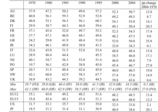
Over the past three decades public spending has been on an upward trend in the EU15

countries with a significant increase in the expenditures-to-GDP ratio from 1970 until

the beginning of the 1990s, from 35.8 per cent of GDP in 1970 to 51.3 per cent of

GDP in 1995. Expenditure-to-GDP ratios then first decreased to 46.8 per cent in 2000

but increased again to 48.0 per cent in 2004. For instance, the share of expenditures in

GDP for individual countries increased from 32.6, 37.1 and 42.1 per cent respectively

in Italy, France and Sweden in 1970, to 53.8, 49.7 and 58.5 per cent in 1990 (see

Table 1).

Table 1 – Total public expenditure as a % of GDP (General government)

1970 1980 1985 1990 1995 2000 2004 pp change

2004-1970

AU _{37.9 47.2 50.2 49.6 57.2 52.3 50.7 12.8}

BE _{40.8 56.1 59.3 52.9 52.8 49.2 49.5 8.7}

DK _{40.8 53.1 56.3 56.1 60.3 54.1 55.0 14.1}

FI _{29.9 38.7 44.3 46.0 59.6 49.1 50.4 20.5}

FR _{37.1 45.4 52.0 49.7 55.2 52.5 54.5 17.4}

GE _{37.7 47.1 46.0 44.1 49.6 48.2 47.5 9.8}

GR _{24.2 29.0 41.9 48.4 51.0 52.0 50.0 25.8}

IR _{34.2 46.1 49.0 38.0 41.5 32.0 34.3 0.1}

IT _{32.6 43.0 51.5 53.8 53.4 48.0 48.4 15.8}

LU _{28.9 48.4 44.4 45.5 38.5 46.0 17.1}

NE _{40.1 54.7 56.3 53.0 51.4 46.0 48.0 7.9}

PO _{19.7 36.1 42.8 38.8 45.0 45.4 46.7 27.0}

SP _{20.7 31.5 40.4 42.6 45.0 40.0 40.5 19.8}

SW 42.1 60.0 62.9 58.5 67.7 57.4 57.0 14.9

UK _{36.9 43.2 44.3 39.2 44.5 39.8 43.6 6.6}

Min 19.7 (PO) 29.0 (GR) 40.4 (SP) 38.0 (IR) 41.5 (IR) 32.0 (IR) 34.3 (IR) 0.1 (IR)

Max 42.1 (SW) 60.0 (SW) 62.9 (SW) 58.5 (SW) 67.7 (SW) 57.4 (SW) 57.0 (SW) 27.0 (PO)

EU12 35.1 45.0 49.2 48.2 51.6 48.2 48.5 13.4 EU15 35.8 45.4 49.1 47.4 51.3 46.8 48.0 12.2

US _{31.7 33.1 35.7 35.5 35.0 32.5 33.8 2.1}

JP _{18.5 31.2 31.4 31.1 36.9 40.9 38.6 20.1}

Source: AMECO Database, updated on 4 April 2005.

Up to 1995 expenditures-to-GDP ratios kept on rising for most countries, reaching

more than half of GDP for nine EU countries and going above 60 per cent of GDP for

Sweden and Denmark. The aforementioned general trend in public expenditures is

reflected in the overall increase of 12.2 percentage points of GDP for the EU15

(12)

increase in Ireland to a maximum increase of 27 percentage points of GDP in

Portugal.

Nevertheless, the limitations imposed by sustainability of public finances led most EU

countries to curb down expenditure growth from the mid-1990s onwards. Indeed, the

expenditure-to-GDP ratio in the EU15 was reduced from 51.3 per cent in 1995 to 46.8

per cent in 2000, halting therefore the raising trend of public expenditures in the EU.

More particularly, the ratio of public expenditures-to-GDP declined between 1995

and 2000 for all EU countries, with the exception of Greece and Portugal, where that

ratio increased by 1.0 and 0.4 percentage points of GDP respectively. Additionally,

France and Germany had the lowest decreases of the expenditures-to-GDP ratio

between 1995 and 2000, respectively 2.5 and 1.4 percentage points (pp) of GDP while

the overall reduction was 3.4 pp of GDP in the EU12 and 4.5 pp of GDP in the EU15.

On the other hand only two countries in the EU reported an increase of the respective

expenditure-to-GDP ratio between 1995 and 2004: Luxembourg and Portugal (see

Table 1).

The increase in total expenditures must be seen against a background where

governments gradually tried to focus economic policy towards a better fulfilment of

the usually defined “Musgravian” goals: macroeconomic stabilisation, income

redistribution, and more efficient resource allocation.1 In fact, it was during the 1970s and 1980s that most industrialised countries increased the coverage of social

programmes such as unemployment insurance. On the other hand, pensions related to

public pension programmes, even if introduced in the end of the 19th in Germany, France and Italy were also reinforced in the 1970s and in the 1980s in most European

countries. Additionally, population ageing played a major role in pushing up these

spending items.

The increase in social transfers in the EU15, during the 1970s and 1980s (some 5 pp

of GDP between 1970and 1990 for the EU15), was generalised to every country.

Moreover, for the period 1970-2004 significant increases were recorded in the social

1

(13)

transfers-to-GDP ratio in Portugal (11.3 pp), Greece (10.2 pp), Finland (8.8 pp),

Denmark and Sweden (6.9 pp), and Germany (6.6 pp).

Regarding another important current expenditure category, compensation of

employees, its share in GDP increased roughly 1.1 percentage points of GDP for the

EU15 countries, between 1970 and 2004. Nevertheless, it is important to mention the

existence of large differences both among countries and through time in this

expenditure category. For instance, one can notice that the compensation of

employees as a share of GDP in 1980 ranged from to 9.4 per cent in Greece and Spain

to 18.0 and 20.2 per cent in Denmark and Sweden. On the other hand, in 2004 the

lower values for those ratios were 7.6, 8.6 and 8.7 per cent respectively in Germany,

Luxembourg and Ireland, while the higher reported values were 13.8 per cent in

Finland, 14.7 per cent in Portugal, 16.3 per cent in Sweden and 17.8 in Denmark.

In spite of the moderate general increase in the share of compensation of employees in

GDP, in the EU15, that ratio did increase more significantly in six countries: Portugal,

Denmark, Greece, Spain, Finland, and France. The biggest increases during that

period occurred in Portugal, Denmark and Greece, with respectively changes of 7.5,

4.4 and 4.3 percentage points. On the other hand, compensation of employees as a

share of GDP decreased between 1970 and 2004 in three countries: Ireland, Germany

and Austria, and remained at the same level in the UK.

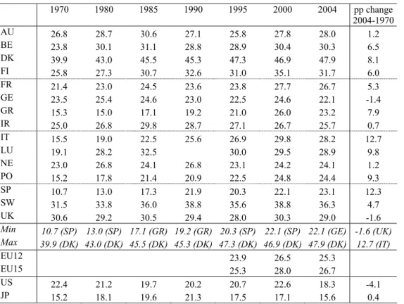
2.2. General government revenues in the EU

During the last four decades tax revenues as a share of GDP increased in most

countries of the EU, as can be seen from Table 2. For instance, this was notably the

case of Italy, Spain, Luxembourg, and Portugal, where the aforementioned ratio

increased by more than nine percentage points. Small decreases in the tax burdens

were observed throughout that period in the UK and in Germany. In 2004 the tax

burden ranged from a minimum of 22.1 per cent in Germany to 47.9 per cent in

Denmark. Indeed, Denmark alongside with Sweden always depicted tax revenues

(14)

Table 2 – Tax revenues as a % of GDP (General government)

1970 1980 1985 1990 1995 2000 2004 pp change

2004-1970

AU _{26.8 28.7 30.6 27.1 25.8 27.8 28.0 1.2}

BE _{23.8 30.1 31.1 28.8 28.9 30.4 30.3 6.5}

DK _{39.9 43.0 45.5 45.3 47.3 46.9 47.9 8.1}

FI _{25.8 27.3 30.7 32.6 31.0 35.1 31.7 6.0}

FR _{21.4 23.0 24.5 23.6 23.8 27.7 26.7 5.3}

GE _{23.5 25.4 24.6 23.0 22.5 24.6 22.1 -1.4}

GR _{15.3 15.0 17.1 19.2 21.0 26.0 23.2 7.9}

IR _{25.0 26.8 29.8 28.7 27.1 26.7 25.7 0.7}

IT _{15.5 19.0 22.5 25.6 26.9 29.8 28.2 12.7}

LU _{19.1 28.2 32.5 30.0 29.5 28.9 9.8}

NE 23.0 26.8 24.1 26.8 23.1 24.2 24.1 1.2

PO _{15.2 17.8 21.4 20.9 22.5 24.8 24.4 9.3}

SP _{10.7 13.0 17.3 21.9 20.3 22.1 23.1 12.3}

SW _{31.5 33.8 36.0 38.8 35.6 38.8 36.3 4.7}

UK _{30.6 29.2 30.5 29.4 28.0 30.3 29.0 -1.6}

Min _{10.7 (SP) 13.0 (SP) 17.1 (GR) 19.2 (GR) 20.3 (SP)} _{22.1 (SP) 22.1 (GE) -1.6 (UK)}

Max _{39.9 (DK) 43.0 (DK) 45.5 (DK) 45.3 (DK) 47.3 (DK) 46.9 (DK) 47.9 (DK) 12.7 (IT)}

EU12 _23.9_26.5_25.3

EU15 _25.3_28.0_26.7

US _{22.4 21.2 19.7 20.2 20.7 22.6 18.3 -4.1}

JP _{15.2 18.1 19.6 21.3 17.5 17.1 15.6 0.4}

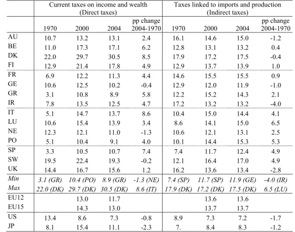
Source: AMECO Database, updated on 4 April 2005. Total taxes include: current taxes on income and wealth (direct taxes), and taxes linked to imports and production (indirect taxes).

Additionally, it is also possible to notice that the share of direct taxes in GDP for

individual countries increased between 1970 and 2004 for all EU countries with the

exception of the Netherlands, Germany and Sweden where decreases were reported

(see Table 3). In 2004 the direct taxes-to-GDP ratio ranged from 8.9 per cent in

(15)

Table 3 – Direct and indirect taxes as a % of GDP (General government)

Current taxes on income and wealth (Direct taxes)

Taxes linked to imports and production (Indirect taxes)

1970 2000 2004 pp change

2004-1970 1970 2000 2004

pp change 2004-1970

AU _{10.7 13.2 13.1 2.4 16.1 14.6 15.0 -1.2}

BE _{11.0 17.3 17.1 6.2 12.8 13.1 13.2 0.4}

DK _{22.0 29.7 30.5 8.5 17.9 17.2 17.5 -0.4}

FI _{12.9 21.4 17.8 4.9 12.9 13.7 13.9 1.0}

FR _{6.9 12.2 11.3 4.4 14.6 15.5 15.5 0.9}

GE _{10.6 12.5 10.2 -0.4 12.9 12.0 11.9 -1.0}

GR _{3.1 10.8 8.9 5.8 12.2 15.2 14.3 2.1}

IR _{7.8 13.5 12.5 4.7 17.2 13.2 13.2 -4.0}

IT _{5.1 14.7 13.7 8.6 10.4 15.0 14.4 4.1}

LU _{10.6 15.4 13.9 3.4 8.6 14.1 15.0 6.5}

NE _{12.3 12.1 11.0 -1.3 10.6 12.1 13.1 2.5}

PO _{5.1 10.4 9.1 4.0 10.1 14.4 15.3 5.3}

SP _{3.3 10.5 10.7 7.4 7.4 11.7 12.4 4.9}

SW _{19.5 22.4 19.3 -0.2 12.1 16.4 17.0 4.9}

UK _{14.4 16.7 15.6 1.2 16.2 13.6 13.4 -2.8}

Min _{3.1 (GR) 10.4 (PO) 8.9 (GR) -1.3 (NE)} _{7.4 (SP)} _{11.7 (SP) 11.9 (GE) -4.0 (IR)}

Max _{22.0 (DK) 29.7 (DK) 30.5 (DK)} _{8.6 (IT)} _{17.9 (DK) 17.2 (DK) 17.5 (DK) 6.5 (LU)}

EU12 _13.0_{11.7 13.6}_13.6

EU15 _14.3_{13.0 13.7}_13.7

US _{13.4 8.6 7.3 -0.8 8.9 7.3 7.2 -1.7}

JP _{8.1 15.4 11.1 -2.3 7. 8.4 8.3 -1.2}

Source: AMECO Database, updated on 4 April 2005. Direct taxes – current taxes on income and wealth. Indirect taxes – taxes linked to imports and production.

Moreover, the share of indirect taxes in GDP for individual countries also increased

between 1970 and 2003 for most EU countries with the exception of five countries:

Austria, Denmark, Germany, Ireland and the UK (see also Table 3). In 2004 the

indirect taxes-to-GDP ratio ranged from 11.9% in Germany to 17.5 per cent in

Denmark.

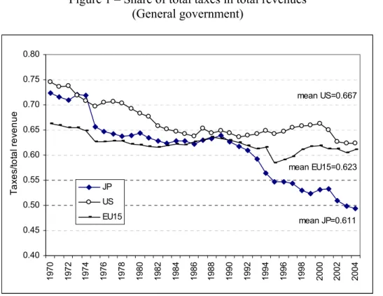
Another relevant measure concerns the share of total taxes in total revenues. The

developments of such ratio are illustrated in Figure 1 for the EU15 (simple average),

Japan and the US. The average share of tax revenues in the general government total

revenues in this period, ranged from 0.515 in France and Spain to 0.848 in Denmark.

The comparable ratio for the EU15 averaged 0.623 in 2004, encompassing a

minimum of 0.584 in 1995 and a maximum of 0.662 in 1970. Those developments in

terms of the average EU15 are not very different from the ones observed in the US,

(16)

Figure 1 – Share of total taxes in total revenues (General government)

mean JP=0.611 mean US=0.667

mean EU15=0.623

0.40 0.45 0.50 0.55 0.60 0.65 0.70 0.75 0.80

1970 1972 1974 1976 1978 1980 1982 1984 1986 1988 1990 1992 1994 1996 1998 2000 2002 2004

T

a

xe

s/

to

ta

l re

ve

n

u

e

JP

US

EU15

Source: AMECO database, updated on 4 April 2005.

Regarding social security contributions, which are also a major source of financing

for general government, Table 4 summarises the relevant developments for the EU15.

It is possible to see that throughout the 1970-2004 period social security contributions

as a share of GDP increased for all EU15 countries, as well in Japan and in the US.

The development in the social security contributions-to-GDP ratio was not

homogeneous for the EU countries in the last years. Indeed, significant rises occurred

between 1970-2004 for the cases of Greece, Portugal, and Spain, respectively 8.6, 7.6,

and 6.2 pp. On the other hand, more mitigated increases were seen in the cases of the

UK, Netherlands, and Luxembourg, while this ratio is quite small in Denmark (where

taxes-to-GDP ratios are nevertheless quite above average). If one looks at a more

recent period, say between 1995 and 2004, similar patterns emerge regarding the

countries where social security contributions share increased, notably Greece,

Portugal and Sweden. However, in this case, the main reductions were reported for

(17)

Table 4 – Social security contributions (General government)

1970 1980 1985 1990 1995 2000 2004 pp change

2004-1970

AU _{10.7 14.6 14.8 15.3 17.3 16.8 16.4 5.7}

BE _{12.0 14.9 17.1 16.8 16.8 16.1 16.0 4.0}

DK _{2.4 1.8 2.8 2.3 2.6 3.3 2.7 0.3}

FI _{5.5 10.9 11.4 12.8 14.8 12.3 12.0 6.4}

FR _{13.8 19.1 20.8 20.6 20.5 18.2 18.2 4.4}

GE _{12.3 16.6 17.1 16.5 18.8 18.6 18.2 5.9}

GR _{7.7 9.4 11.6}_11.5_{12.6 14.0 16.3 8.6}

IR _{2.3 4.4 5.1 5.0 6.8 5.7 6.2 3.9}

IT _{11.2 12.9 13.5 14.3 14.8 12.7 12.9 1.8}

LU _{8.6 13.4 12.4 12.5 11.2 12.2 3.6}

NE _{13.1 17.5 19.8 16.4 17.2 17.1 15.1 2.0}

PO _{5.1 7.9 8.6 10.1}_{11.0 11.8 12.7 7.6}

SP _{7.4 12.6 12.7 12.9 13.0 13.3 13.6 6.2}

SW _{8.6 14.7 13.5 14.9 13.7 15.0 14.7 6.1}

UK _{5.2 6.0 6.8 6.2 7.5 7.6 8.1 2.9}

Min _{2.3 (IR)} _{1.8 (DK)} _{2.8 (DK)} _{2.3 (DK)} _{2.6 (DK)} _{3.3 (DK)} _{2.7 (DK)} _{0.3 (DK)}

Max _{13.8 (FR) 19.1 (FR) 20.8 (FR) 20.6 (FR) 20.5 (FR) 18.6 (FR) 18.2 (FR)} _{8.6 (GR)}

EU12 _17.4_16.2_15.9

EU15 _15.7_14.3_14.3

US _{4.5 6.0 6.7 7.1 7.3 7.2 7.0 2.5}

JP _{4.3 7.3 8.1 8.9 9.3 9.8 10.9 6.6}

Considering the magnitude of tax revenues, including also social security

contributions, the effort supported by the EU15 was 40.9 per cent of GDP in 2004

(see Table 5), which compares with ratios of 25.3 per cent and 26.5 per cent

respectively in the US and in Japan. During the period 1970-2004 one can notice

significant increases in the share of taxes and social security contributions in GDP for

several countries, notably in Spain, Portugal, Greece, and Italy, respectively 18.5,

16.9, 16.4, and 14.5 pp. On the other hand, the smallest increases were recorded for

(18)

Table 5 – Tax revenues including social security contributions (General government)

1970 1980 1985 1990 1995 2000 2004 pp change

2004-1970

AU _{37.5 43.3 45.5 42.4 43.1 44.6 44.4 6.9}

BE _{35.8 45.0 48.2 45.7 45.7 46.5 46.4 10.6}

DK _{42.3 44.8 48.3 47.6 49.9 50.1 50.7 8.4}

FI _{31.3 38.2 42.1 45.4 45.8 47.4 43.7 12.4}

FR _{35.3 42.1 45.3 44.2 44.3 45.8 45.0 9.7}

GE _{35.9 42.0 41.8 39.4 41.3 43.2 40.3 4.5}

GR _{23.1 24.4 28.7 30.8 33.5 40.0 39.5 16.4}

IR _{27.3 31.2 35.0 33.6 34.0 32.4 31.9 4.6}

IT _{26.6 32.0 36.0 39.9 41.7 42.5 41.1 14.5}

LU _{27.7 41.6 44.9 42.5 40.7 41.1 13.4}

NE _{36.0 44.2 44.0 43.2 40.4 41.3 39.3 3.2}

PO _{20.2 25.7 30.0 31.0 33.4 36.6 37.1 16.9}

SP _{18.1 25.6 30.0 34.8 33.3 35.4 36.7 18.5}

SW _{40.2 48.5 49.5 53.7 49.4 53.8 51.0 10.8}

UK _{35.8 35.3 37.3 35.6 35.5 37.8 37.0 1.3}

Min _{18.1 (SP) 24.4 (GR) 28.7 (GR) 30.8 (GR) 33.3 (SP)} _{32.4 (IR) 31.9 (IR)} _{1.3 (UK)}

Max _{42.3 (DK) 48.5 (SW) 49.5 (SW) 53.7 (SW) 49.9 (DK) 53.8 (SW) 51.0 (SW) 18.5 (SP)}

EU12 _41.3_42.7_41.2

EU15 _41.0_42.3_40.9

US _{26.9 27.2 26.4 27.3 27.9 29.8 25.3 -1.6}

JP _{19.5 25.3 27.7 30.1 26.7 26.9 26.5 7.0}

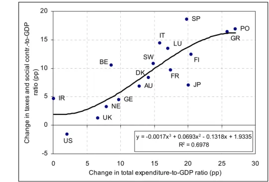
Additionally, still another relevant stylised fact, which is worthwhile mentioning, is

the positive and quite relevant relation that one can visually observe in Figure 2,

between the change in the total spending-to-GDP ratio and the change in the taxes and

social contributions-to-GDP ratio, in the last four decades. Therefore, this somehow

points to the existence of a long-term relationship between total spending and tax

(19)

Figure 2 – Changes in total spending and in taxes and social contributions-to-GDP ratios, between 1970 and 2004

UK GE NE AU JP SW FR FI GR PO US LU SP IT DK IR BE

y = -0.0017x3_{+ 0.0693x}2_{- 0.1318x + 1.9335} R2_{= 0.6978}

-5 0 5 10 15 20

0 5 10 15 20 25 30

Change in total expenditure-to-GDP ratio (pp)

C ha nge in t ax es an d s oc ia l c ont r. -t o-G D P ra ti o (p p )

Source: Tables 1 and 5.

All in all, the stylised evidence reviewed in this section cannot be overlooked as a

reinforcement of the conclusion that, as expected, regardless of public spending being

carried out either efficiently or inefficiently, the underlying financing relies on taxing

the economy. Moreover, the reliance on tax revenues seems to be rather stable

throughout the period and across the EU countries, while it is interesting to notice that

social security contributions decreased as a ratio to GDP between 1995 and 2004, for

the EU as a whole.

3. Inefficiency in the provision of public services

3.1. The theoretical production possibility frontier

Much has been published recently on efficiency and effectiveness in the provision of

public services. The topic is naturally important in many different ways. However, for

the purpose of our paper, it suffices to single out a single parameter, measuring

efficiency in public services provision. In doing so, we follow Afonso, Schuknecht

and Tanzi (2005, 2006). On the basis of cross-country data, for 23 OECD, countries

Afonso, Schuknecht and Tanzi (2005) use a non-parametric approach to compute a

(20)

public sector spending. Their efficiency score indicator δ varies from 0 to 1. It is unity for combinations of spending and performance on the production possibility frontier.

For combinations inside the frontier the efficiency score indicator is smaller than 1.

Specifically, δ<1, and from an input orientation perspective,means that the country could provide the same amount of public services with δ per cent of the resources used, if it would move to the efficiency frontier. In other words, assuming that a

country could (conceivably) provide a given amount of public sector services on the

efficiency frontier, then δ<1 means that, in actual practice, that country is spending 1/δ times the minimum required. That requires 1/δ times more resources.

Figure 3 displays an example of a production possibility frontier with decreasing

returns to scale for the output level Y and cost level X. For instance, countries A and C are efficient, with δ=1, while a country such as B is inefficient (δ<1), since it lies inside the frontier. Indeed, country B may be considered inefficient, in the sense that

it performs worse than country C, because we have Y(B)<Y(C) and X(B)>X(C). Therefore, country C achieves a better status with less expenditure.

(21)

Still from Figure 3 we can see that (Y*, X*) is efficient in the sense that it is impossible to decrease the resources used while maintaining the same output level.

On the contrary, (Y*, X(B)) is inefficient since X(B)/X*=1/δ, which is above one, that is, displays excess use of resources. Maintaining Y fixed at the level of Y* it is clear that inefficiency requires the public sector to raise (1/δ-1)X* extra revenues. In other words, (1/δ-1)X* is a measure of the direct cost of inefficiency in the provision of public services, and an actual government spends 1/δ times more than the minimum required. Clearly, (1/δ-1) measures, in Pigou’s terminology, the direct cost of public sector inefficiency. For example, Afonso, Schuknecht and Tanzi (2005) estimate that,

for instance, the input efficiency score δ is 0.79 for Portugal (see next subsection). It means that the country is using 26.6 per cent more resources than the minimum

required to provide the current amount of public services.2

The question that naturally follows is: are the direct costs of inefficiency a good

measure of the total cost imposed on the economy? Is it a good approximation? In this

paper, following the tradition of Dupuit and Pigou, we will investigate whether

indirect costs are relevant and by how much relevant.

For the purpose of our discussion we will rely on a powerful simplifying assumption

taking the basket of public services as invariant. For example, in Figure 3, we take

public services output as fixed at the level Y*. Thus, we can completely avoid questions about what are the effects of public services on private expenditures, about

whether public services are worthwhile and many more. Our analysis focuses

exclusively on the financing side. In this paper, we will take into account the budget

constraint of the public sector. In other words we will make it explicit that public

sector expenditure must be financed by taxation.3

2

In Afonso, Schuknecht and Tanzi (2006), using a different sample of countries, the authors report an estimated δ of 0.385, for Portugal. Such estimate implies that the country is using 159 per cent more resources than the minimum necessary to provide the same bundle of public services (see Table 7 below).

3

(22)

In order to address these questions it is necessary to model the household sector of the

economy in some detail. However, a much stylised representation of the production

side will suffice. Specifically, we follow the standard set of assumptions in the

literature and assume that a single representative household can represent the

consumption sector and that the economy’s production possibilities can be captured

by a linear technology. In particular, we will assume a single production factor,

labour, and constant returns to scale. Finally, and most importantly, we will assume

that lump sum taxation is not institutionally feasible. Only economic transactions can

be taxed. Work and consumption can be taxed while leisure cannot4.

We will compare a situation where the public sector has to raise R*=X* in taxes with a situation where the public sector is inefficient and must therefore raise R=X(B) in taxes, for the example in Figure 3. Therefore, we know that (R-R*)=(1/δ-1)R*.

Now it is clearly true that there are many ways to raise additional resources. So it

seems that we cannot make further progress without adding some assumption about

the structures of taxation and how it changes in order to obtain extra revenues. One

possibility would be to assume that the structure of taxation is optimal. Such

assumption is workable but it seems to us, unrealistic. Thus, we assume instead that

there is some initial structure of taxation and that the government raises additional

revenue simply by changing the tax structure in a proportional way (in section 2.2 we

saw from historical data for the EU that this is not too far from reality). Such

assumption, we agree, is not only natural but allows us to simplify our problem

tremendously. This is so because the restriction we impose on the tax structure,

combined with our assumptions about technology, allows us to apply the composite

commodity theorem (of Hicks (1936) and Leontief (1936)). As we will show in the

next sub-section, under our set of assumptions the financing problem of the

government collapses into the choice of a single tax rate.

4

(23)

3.2. Efficient provision of public services: some evidence

In this section we report on some of the available evidence in the literature regarding

public sector efficiency in the provision of public services. From such evidence we

can afterwards assess the plausibility of the magnitude of inefficiency to use ahead in

the numerical simulations in section five.

In order to compute a composite indicator of public sector performance for OECD

countries, Afonso, Schuknecht and Tanzi (2005) use several sub-indicators of public

performance that take into account, for instance, administrative, education, health and

public infrastructure outcomes. They also look at other indicators to incorporate

information on the usually defined “Musgravian” functions of the government:

macroeconomic stabilisation, income redistribution and efficient resource allocation.

The so-called performance indicators are compiled from various indices that have

each an equal weight. Based on that performance indicator as an output measure, they

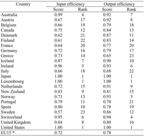
computed efficiency scores, which we reproduce in Table 6.

The average input efficiency of the EU15 countries is 0.72 meaning that they should

be able to attain the same level output using only 72 per cent of the inputs they are

currently using. In other words, on average, the sample countries are using 38.9 per

cent more resources than the minimum required to provide the same amount of public

(24)

Table 6 – Public sector efficiency scores: 2000

Country Input efficiency Output efficiency

Score Rank Score Rank

Australia 0.99 4 0.92 7

Austria 0.67 17 0.92 8

Belgium 0.66 19 0.79 18

Canada 0.75 12 0.84 13

Denmark 0.62 21 0.87 11

Finland 0.61 22 0.83 14

France 0.64 20 0.77 20

Germany 0.72 16 0.79 17

Greece 0.73 14 0.65 23

Iceland 0.87 7 0.90 10

Ireland 0.96 5 0.93 6

Italy 0.66 18 0.68 22

Japan 1.00 1 1.00 1

Luxembourg 1.00 1 1.00 1

Netherlands 0.72 15 0.91 9

New Zealand 0.83 9 0.81 15

Norway 0.73 13 0.93 5

Portugal 0.79 11 0.70 21

Spain 0.80 10 0.78 19

Sweden 0.57 23 0.86 12

Switzerland 0.95 6 0.94 4

United Kingdom 0.84 8 0.80 16

United States 1.00 1 1.00 1

EU15 * 0.72 0.78

Source: adapted from Afonso, Schuknecht and Tanzi (2005), Free Disposable Hull scores. * - Weighted averages according to the share of each country GDP in the EU15.

The average output efficiency score of the EU15 implies that with given public

expenditures, public sector performance is 78 percent (or 22 percent less) of what it

could be if the EU15 was on the production possibility frontier (and more if the

countries on the production possibility frontier also have scope for expenditure

savings).

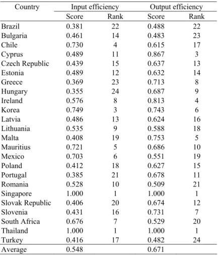
Afonso, Schuknecht, and Tanzi (2006) provide another set of efficiency calculations,

for the new EU member states and for a set of mostly emerging markets. We report

(25)

Table 7 – Public sector efficiency scores: 2001/2003

Input efficiency Output efficiency Country

Score Rank Score Rank

Brazil 0.381 22 0.488 22

Bulgaria 0.461 14 0.483 23

Chile 0.730 4 0.615 17

Cyprus 0.489 11 0.867 3

Czech Republic 0.439 15 0.637 13

Estonia 0.489 12 0.632 14

Greece 0.369 23 0.713 8

Hungary 0.355 24 0.687 9

Ireland 0.576 8 0.813 4

Korea 0.749 3 0.743 6

Latvia 0.486 13 0.624 16

Lithuania 0.535 9 0.588 18

Malta 0.408 19 0.753 5

Mauritius 0.721 5 0.686 10

Mexico 0.703 6 0.551 19

Poland 0.412 18 0.627 15

Portugal 0.385 21 0.678 11

Romania 0.528 10 0.509 21

Singapore 1.000 1 1.000 1

Slovak Republic 0.406 20 0.674 12

Slovenia 0.431 16 0.731 7

South Africa 0.676 7 0.529 20

Thailand 1.000 1 1.000 1

Turkey 0.416 17 0.482 24

Average 0.548 0.671

Source: adapted from Afonso, Schuknecht and Tanzi (2006). Variable returns to scale efficiency scores, via Data Envelopment Analysis.

Interestingly, one can notice, for instance, that countries like Greece and Portugal,

which are present in both the results of Table 6 and 7, come out as less efficient in the

second subset in terms of input efficiency (even if the underlying variables are not

totally comparable). In practice, and due to the fact of differences in relative prices in

the provision of public services, notably regarding compensation of employees, what

one can guess is that, for such countries, the efficiency scores from Table 6 could be

overestimated while the efficiency scores from Table 7 may be underestimated. All in

all, and as a tentative assessment, this could provide a possible range for the input

efficiency scores for countries present in both samples.

Inspired on the analysis of Afonso, Schuknecht, and Tanzi (2005), additional the

Social and Cultural Planning Office (SCP) of the Netherlands (2004) provides also

(26)

four new members of the EU, Czech Republic, Hungary, Poland and Slovakia,

alongside with the EU15. In line with Afonso et al. (2005), they use 19 indicators

divided into four main groups: stabilisation/growth, distribution, allocation and

quality of public administration.

The results reported by the SCP (2004) seem to point to the fact that there isn’t much

relation between public performance and public spending. The best performers are

Ireland, Finland and Luxembourg. Good performers are also Sweden, Denmark,

Austria, and the Netherlands. Most southern European countries, notably Portugal,

Greece and Italy, and also Hungary, show below average performance and average

public spending. All in all, both set of results point to the existence of relevant

inefficiencies in the provision of public services.5

In this paper, we will not take a stand on the accuracy and reliability of the available

estimates. Instead, we will use the range of input efficiency estimates, for Portugal,

from Afonso, Schuknecht and Tanzi (2005, 2006), for the numerical examples of

subsection 4.2.

4. The simplest theoretical framework

Here we review some of the theoretical underpinnings. We will explore the costs

associated with the financing of inefficiency in public services provision through

distortional taxation. We will use Hicks’ compensating variation (following Diamond

and McFadden (1974) and Auerbach (1985)) to show that these magnification

mechanisms are not only conceptually relevant, they are also important from a

quantitative point of view. Specifically, we rely on a range of estimates of public

sector efficiency (from Afonso, Schuknecht and Tanzi (2005, 2006) to illustrate

numerically that the relative importance of indirect costs of public sector provision

inefficiency, linked to financing through distortional taxation, increases with the

magnitude of the inefficiency.

5

(27)

4.1. Direct and indirect costs of inefficiency

Under our assumptions, consumer choices may be summarized (without loss of

generality) as involving only two goods (consumption and leisure). In such a setting,

without any external source of income, the household budget constraint is

) )( 1 ( )

1

( +tc px=w −tl T −l , (1)

where tc is the tax rate on consumption, p is the producer price of the consumption good (assumed fixed by perfect competition and linear technology), x is consumption,

w the gross wage rate, tl the tax on work, T is the time endowment (given) and, finally, l is leisure.

Thus there is no loss of generality in writing:

) ( 1

1

l T w px t t

l c

− = −

+

, (2)

or simply

) ( ) 1

( +t px= T −l , (3)

where (1+t)=(1+tc)/(1-tl) and we take leisure (or work) as the numeraire (that is we take w=1)6. Equation (3) may be written in compact form as

) (T l

qx= − , (4)

where q=(1+t)p.

Such form is frequently used in the optimal taxation literature where q denotes consumer prices and p denotes producer prices.

6

Alternatively equation (3) could be written as: px=(1−τ)(T−l)where

t t

+ =

1

(28)

Formulated in these terms our problem becomes very simple and can be approached

following the methodology in Diamond and McFadden (1974) and Auerbach (1985).

For our specific case it implies the following steps:

First, we take a situation of efficiency in public services’ provision as our starting

point. In other words we will consider a pair (Y0, X0) in the production possibility frontier in Figure 3. The necessary resources X0 correspond exactly to the tax revenues collected:

) , ) 1 (( )

0 , ) 1

(( 0 0 0 0

0 0

0 _R _t _x _t _p _t _h _t _p _u

X = = + = + . (5)

It is true that

0 ) , ( ) , ) 1

(( +t0 p u0 =e q0 u0 =

e , (6)

where x(.) is the Marshallian demand function; h(.) the Hicksian demand function and

e(.) the expenditure function. u0 denotes the utility that the representative consumer attains when the provision of public services Y0 is done efficiently. Equation (6) is implied by our simplifying assumption that all of the income, obtained by our representative consumer, derives from work effort. In other words, we assume that

there is no lump sum income, when public services provision is done efficiently.

As we have seen before if provision is inefficient it is necessary to raise additional

revenue:

δ

0

1 R

R = . (7)

In order to raise R1 the government – in the model – will have to increase taxes. To ensure consistency with the measures of welfare change that we will propose to use

(29)

using the Hicksian demand function. The level of utility to use will be u0, exactly the level that the representative consumer will attain under efficient provision.

Thus, to wrap up the new required level of taxation will have to satisfy:

) , ) 1 (( )

, ) 1

(( 1 0 1 1 0

0 1

u p t ph t u p t R R

R = = + = +

δ , (8)

where R is the tax revenue function as in Diamond and McFadden (1974). Hence, the second step, in our procedure, is to determine the tax rate, t1 that is necessary to balance the budget under the relevant degree of inefficiency in public service

provision.

Figure 4 allows a simple graphical explanation of the loss, in consumption terms, for

the consumer, associated with inefficiency in public services’ provision.

(30)

In Figure 4 our starting point, E0, satisfies e((1+t0)p,u0)=0 by construction. If one

would consider only the increase in taxes from t0 to t1, without compensating the consumer, welfare would decline to u1, at point E1. Without compensation,

expenditure – at the new level of welfare – would remain unchanged:

0 ) , ) 1

(( ₊_t1 _p _u1 ₌

e . When taxation increases, as required by inefficiency in public services’ provision, the consumer must be compensated, in order to be able to attain

the initial level of utility. When such compensation is paid, the budget constraint

shifts up, and the corresponding equilibrium is labelled E2 in Figure 4. The increase

in taxation is thus associated with a total loss (as measured by Hicks’ compensating

variation), in terms of consumption, of OQ, of which OQL is the change in the

deadweight loss while QLQ is the additional tax revenue.

In other words, in order to quantify (in monetary units) the consumer’s welfare we

take the level of utility u0 and ask: how much would it be necessary to pay the consumer so that she would be able to reach the initial level of welfare when taxes are

increased from t0 to t1? The answer is given by the compensating variation, CV:

), , ) 1 (( ) , ) 1 (( ) , ) 1 (( ) , ) 1 (( 1 1 0 1 0 0 0 1 u p t e u p t e u p t e u p t e CV + − + = = + − + = (9)

where the latter equality makes it clear that the compensating variation measures

welfare change, in the monetary units, evaluated at the consumer prices prevailing in

the after tax increase situation.

Therefore, ⎟ ⎠ ⎞ ⎜ ⎝ ⎛ − −

= ( , , ) 1 1

) , ,

( 1 0 0 1 0 0 0

δ R u t t CV u t t

L , (10)

is our measure of deadweight loss or excess burden. Thus the third and last step in our

procedure is to compute the compensating variation and the corresponding measure of

(31)

4.2. Costs of inefficiency in public services provision

In order to make our procedure operational, it is necessary to make assumptions about

consumer preferences and constraints. In this subsection we provide some estimates

of using a simple parameterised example based on the linear expenditure system

(Stone-Geary preferences):7

) ( )

( ₁ 1

0 0 γ α

γ α −

−

= l x

U . (11)

The indirect utility function for the Stone-Geary preferences v(.) is given by

{

l x T l x t px T l

}

l x t

p

v + = ( − ) ( − ) : ≥ ≥ ≥0; ≥ ≥0;(1+ ) = −

, max ) 0 , 1 ), 1 (

( ₁ 1 ₀ ₁

0 0 γ α γ γ

γ α . (12)

By assumption, we have α0 +α1=1. It is easy to show that the Marshallian demand

functions corresponding to the solution to the above problem, taking into account the

household budget constraint (3), may be written as:8

) ) 1 (

( ₀ ₁

0

0 α γ γ

γ T p t

l = + − − + , (13)

) ) 1 ( ( ) 1

( 0 1

1

1 γ γ

α

γ T p t

t p

x − − +

+ +

= . (14)

It is possible to use the Marshallian demand equations to substitute for x and l in the utility function obtaining the indirect utility function defined above. The indirect

utility function, in turn may be inverted to obtain the corresponding expenditure

function: U t p t p T U t p e 1 0 1 1 0 1 0 ) 1 ( ) 1 ( ) , 1 ), 1 (

( _α _α

α

α α γ

γ + + + +

+ − =

+ . (15)

7

See notably Geary (1950-51). 8

(32)

Deriving the expenditure function in order of the consumer price q=p(1+t) allows us to obtain the Hicksian demand for the consumer good:

U t p q u t p e U t p h 1 0 1 1 0 1 1 1 ) 1 ( ) , 1 ), 1 ( ( ) , 1 ), 1 (

( _α _α

α α α α γ − + + = ∂ + ∂ =

+ . (16)

In our example when public services’ provision is efficient the tax rate is t0. Since we will take that situation as our reference situation we will start out

with:e(p(1+t0),1,U0)=0.

We use this condition to determine the reference utility level, U0 in (15). Using this same utility level in (16) we obtain the Hicksian or compensated demand function

corresponding to the financing needs of the public sector under efficiency in the

provision of public services.

We are now ready to follow the procedure described in section 2. The parameters

used in the simulation will be either inspired by some facts about the Portuguese

economy or will be chosen arbitrarily (we will be explicit about all relevant

assumptions made).

For instance, in Portugal, in 2004, tax revenues (including social security

contributions) were 37.1 per cent of GDP (see Table 5) or almost 60 per cent of

private consumption. In Afonso, Schuknecht and Tanzi, (2005, 2006), efficiency in

public service provision, in Portugal, is estimated at, respectively, 0.79 and 0.39. We

use this range to argue that it makes sense to assume that if public service provision

were efficient in Portugal, taxation in the range of 37.5 per cent of consumption

would suffice for its financing. Assuming T=168=7×24 (just a normalization of the time endowment), α0 =α1=1/2, γ0=98 and γ1=5. Thus, given the conventions adopted,

efficient provision of the given amount of public services requires 14.625 monetary

units. Hence, t0 must equal 0.6 (τ=37.5 per cent).

Let us now quantify what happens when the efficiency in public services’ provision

(33)

Their estimate of efficiency delivers δ=0.79, which implies that to maintain the level of provision an increase of (1/0.79)-1=26.6 per cent is required. If we use the

Using the Hicksian or compensated demand curve for consumption it is easy to see

that the tax revenue function implies that the tax rate must increase to approximately

t1=0.795, in the first case (τ=44.3 per cent). Given that the Hicksian demand function is downward slopping the increase in the tax rate required is proportionally greater

than the required increase in tax revenue. Such effect corresponds to the curvature of

the Dupuit-Laffer curve. The effect is evidently more pronounced for the higher

estimate of inefficiency. In this case t1=1.945 (τ=66.0 per cent).

Using the new tax rate in the expenditure function we may now see that the total loss

(direct and indirect) borne by the consumer is 4.64 monetary units. The value of the

loss compares with an increase in tax revenue of 3.89. Given our parameters, taking

into account indirect costs of inefficiency increases the estimated magnitude of the

loss by about 20 per cent. In our second case the total loss to the consumer equals a

much larger 28.8 monetary units, which compares with an increase in tax revenue of

22.9. The indirect costs, associated with the excess burden, are now 26 per cent. Table

8 reports the results for alternative values of efficiency in public services provision.

Table 8 – Numerical simulation for alternative efficiency scores (t0=0.6; τ=37.5%; α0=α1=0.5; γ1=5)

Efficiency score (δ)

t1 τ (%)

Total loss (monetary

units)

Variation in tax revenues (monetary units)

Increase in the estimated magnitude of

loss (%)

1.00 0.600 37.5 0.00 0.00 -

0.79 0.795 44.3 4.64 3.89 19.3

0.70 0.921 47.9 7.54 6.27 20.3

0.65 1.009 50.2 9.53 7.88 21.0

0.60 1.116 52.7 11.87 9.75 21.8

0.55 1.245 55.5 14.67 11.97 22.6

0.50 1.406 58.4 18.07 14.63 23.5

0.45 1.612 61.7 22.27 17.88 24.6

0.39 1.945 66.0 28.84 22.88 26.1

is (1/0.39)-1=156.4 per cent.

(34)

From Table 8 we can clearly discern the importance of Dupuit-Pigou effects. In fact,

we may verify Dupuit’s two general principles of taxation at work: first, the revenue

shortfall associated with inefficiency in the provision of public services demands a

more than proportional increase in tax rates. In Dupuit’s words “The heavier the tax, the less it yields relatively.” Second, the total loss increases significantly faster than the tax rate (“The loss of utility increases with the square of the tax.”)

In our example the magnification of the cost of inefficiency in public sector provision

is always significant and its relative importance increases with the magnitude the

inefficiency. Specifically, as the efficiency coefficient declines from 0.79 to 0.39, the

relative importance of indirect costs on total costs increases from 19.3 to 26.1 per

cent. In general, as the provision of public services and the degree of inefficiency

increase the more important it becomes to take the indirect costs of provision, through

distortional taxation, into account.

In order to assess the sensitivity of our numerical simulations, we report in Table 9 an

alternative case, where the consumer has a higher preference for leisure, with α0=0.6.

Table 9 – Numerical simulation for alternative efficiency scores (t0=0.6; τ=37.5%; α0=0.6; α1=0.4; γ1=5)

t1 _τ (%)

units)

loss (%)

1.00 0.600 37.5 0.00 0.00 -

0.79 0.801 44.5 4.01 3.27 22.7

0.70 0.933 48.3 6.53 5.27 23.9

0.65 1.025 50.6 8.26 6.62 24.7

0.60 1.137 53.2 10.29 8.20 25.5

0.55 1.274 56.0 12.73 10.06 26.5

0.50 1.446 59.1 15.70 12.30 27.6

0.45 1.666 62.5 19.37 15.03 28.8

0.39 2.025 66.9 25.11 19.24 30.5

Under such conditions, the indirect costs, associated with the excess burden, are now

higher and, for instance, for the case of the lowest efficiency coefficient of 0.39, are

(35)

We report in Table 10 the results for the baseline case using instead γ1=0, which

imposes in this case both a higher tax burden and higher associated costs (see also

Appendix B for additional alternative values attributed to the different parameters,

both with the Stone-Geary function and with a Cobb-Douglas function).

Table 10 – Numerical simulation for alternative efficiency scores (t0=0.6; τ=37.5%; α0=α1=0.5; γ1=0)

t1 τ (%)

units)

loss (%)

1.00 0.600 37.5 0.00 0.00 -

0.79 0.807 44.7 4.39 3.49 25.9

0.70 0.945 48.6 7.18 5.63 27.6

0.65 1.043 51.1 9.10 7.07 28.8

0.60 1.163 53.8 11.38 8.75 30.1

0.55 1.311 56.7 14.13 10.74 31.6

0.50 1.500 60.0 17.50 13.13 33.3

0.45 1.747 63.6 21.72 16.04 35.4

0.39 2.163 68.4 28.42 20.53 38.5

5. Conclusion

In the last four decades there has been a considerable increase in the share of public

expenditures in GDP. It prolongs the trend that goes back at least to the late

nineteenth century (see Tanzi and Schuknecht, 2000). Such pattern has been

accompanied by a substantial increase in public sector revenues, especially derived

from taxation and contributions to social security. The stylised evidence reviewed

documents these dynamics with a special focus on EU countries.

In this paper revisit the literature on the economic consequences from inefficiency in

public services provision. The literature finds that, in many countries, inefficiency in

public services’ provision is considerable. Most authors emphasize the need of

changing public sector management practices and the scope of activities carried out

by general government. Following Dupuit (1844) and Pigou (1947) we focus instead

on the financing side.

The fact that public sector financing must rely on distortional taxation implies that it

(36)

in public services provision. Financing spending through distortional taxation leads to

a magnification of overall costs due to the operation of two general propositions about

taxation, already identified by Dupuit (1844). The first states that it is, in general,

necessary to increase tax rates more than proportionally to the additional revenue

needed due to inefficiency. The second states that the excess burden or deadweight

loss associated with taxation increases with the square of the tax rate. Using simple

numerical examples, using Hicks’ compensating variation (following Diamond and

McFadden (1974) and Auerbach (1985)), and some public sector inefficiency

coefficients form the existing literature, we show that these magnification

mechanisms are not only conceptually relevant, they are also important from a

quantitative point of view.