Bootstrap Panel Granger-Causality Between Government Spending and Revenue

Carlos Pestana Barros & Nicolas Peypoch

A Comparative Analysis of Productivity Change in Italian and Portuguese Airports

WP 006/2007/DE _________________________________________________________

António Afonso and Cristophe Rault

Bootstrap Panel Granger-Causality Between Government Spending and Revenue

WP 39/2008/DE/UECE _________________________________________________________

Department of Economics

WORKING PAPERS

ISSN Nº0874-4548

Bootstrap panel Granger-causality between

government spending and revenue

*

António Afonso

and Christophe Rault

Abstract

Using bootstrap panel analysis, allowing for cross-country correlation, without the need of pre-testing for unit roots, we study the causality between government revenue and spending for the EU in the period 1960-2006. Spend-and-tax causality is found for Italy, France, Spain, Greece, and Portugal, while tax-and-spend evidence is present for Germany, Belgium, Austria Finland and the UK, and for several EU New Member States.

Keywords: panel causality, fiscal policy, EU. JEL: C23, E62, H62.

*

The opinions expressed are those of the authors and do not necessarily reflect those of the ECB or the Eurosystem.

$

ECB, Directorate General Economics, Kaiserstraße 29, D-60311 Frankfurt am Main, Germany. ISEG/TULisbon - Technical University of Lisbon, Department of Economics; UECE - Research Unit on Complexity and Economics; R. Miguel Lupi 20, 1249-078 Lisbon, Portugal. UECE is supported by FCT (Fundação para a Ciência e a Tecnologia, Portugal), financed by ERDF and Portuguese funds. Emails: antonio.afonso@ecb.europa.eu, aafonso@iseg.utl.pt.

#

1. Introduction

Fiscal sustainability studies usually assess the existence of a long-term

cointegration relationship between government revenue and spending.1 Nevertheless,

an important feature linked to the existence of such cointegration relation is the

direction of causality between spending and revenue, which conveys how fiscal policy

is set-up in practice. Indeed, one may have one-way Granger-causality from spending

(revenue) to revenue (spending), i.e. “tax-and-spend” (“spend-and-tax”) causality,

two-way causality or no Granger-causality between revenue and spending.

The literature essentially assesses the existence of causality in a single country

set-up.2 However, there is economic rational for undertaking a panel approach, taking

advantage of non-stationary panel data econometric techniques. In the European

Union (EU), and even if there is no single fiscal policy in place, panel analysis is

relevant in the context of countries seeking to pursue sound fiscal policies within the

framework of the Stability and Growth Pact. Cross-country dependence can be

envisaged in the run-up to Economic and Monetary Union (EMU), via peer pressure

or via integrated financial markets. Moreover, cross-country spillovers in government

bond markets are to be expected, and interest rates comovements inside the EU have

also gradually become more noticeable.

This paper contributes to the literature with a bootstrap panel analysis of

causality between government revenue and spending in the EU country set, to assess

which countries are characterised by a tax-and-spend or by a spend-and-tax behaviour

during the period 1960-2006. Section two explains the methodology, section three

reports the empirical analysis and section four concludes.

1 _{Afonso (2005) explains the relevant linkages and reviews the empirical evidence. Afonso and Rault}

(2007) test the cointegration relationship with panel unit root and cointegration tests, allowing for correlation within and between units.

2

3

2. Series specific panel Granger causality test methodology

We use the panel data approach developed by Kónya (2006), based on a

bivariate finite-order vector autoregressive model, and we apply it in our context to

general government revenue, R, and spending, G: 3

1 2

1 2

1, 1, , , 1, , , 1, ,

1 1

2, 2, , , 2, , , 2, ,

1 1 1,..., 1,..., 1,..., 1,..., i i i i p p

it i i j i t j i j i t j i t

j j

p p

it i i j i t j i j i t j j t

j j

R R G t T i N

G R G t T i N

α β γ ε

α β γ ε

− − = = − − = = ⎧ = + + + = = ⎪ ⎪⎪ ⎨ ⎪ ⎪ _{= + + + = =} ⎪⎩

∑

∑

∑

∑

where the index i

(

)

(

)

the lag, and p1i, p2i and p3i, indicate the longest lags in the system. The error terms,

1, ,i t

ε and ε_{2, ,i t}, are supposed to be white-noises (i.e. they have zero means, constant

variances and are individually serially uncorrelated) and may be correlated with each

other for a given country, but not across countries.

System (1) is estimated by the Seemingly Unrelated Regressions (SUR)

procedure, since possible links may exist among individual regressions via

contemporaneous correlation4 within the two equations. Wald tests for Granger

causality are performed with country specific bootstrap critical values generated by

simulations.

With respect to system (1), in country i there is one-way Granger-causality

from G to R if in the first equation not allγ_1,iare zero but in the second allβ_2,iare zero;

there is one-way Granger-causality from R to G if in the first equation all γ_1,iare zero

3

We are grateful to L. Kónya for providing his TSP codes, which we have adapted for our analysis.

4

but in the second not all β_2,iare zero; there is two-way Granger-causality between R

to G if neither all β_2,inor all γ_1,iare zero; and there is no Granger-causality between R

to G if all β_2,iand γ_1,iare zero.5

This procedure has several advantages. Firstly, it does not assume that the

panel is homogeneous, being possible to test for Granger-causality on each individual

panel member separately. However, since contemporaneous correlation is allowed

across countries, it makes possible to exploit the extra information provided by the

panel data setting. Secondly, it does not require pre-testing for unit roots and

cointegration (since country specific bootstrap critical values are generated), though it

still requires the specification of the lag structure. This is an important feature since

the unit-root and cointegration tests in general suffer from low power, and different

tests often lead to contradictory outcomes. Thirdly, this approach allows detecting for

how many and for which members of the panel there exists one-way, two-way, or no

Granger-causality.

3. Econometric investigation

Data for general government expenditure and revenue are taken from the

European Commission AMECO database.6 The data cover the periods 1960-2006 for

the EU15 countries, and 1998-2006 for the EU25 countries and the unbalanced panels

are used for the SUR analysis and Granger-causality testing.78

5 _{As stressed by Kónya (2006) this definition implies causality for one period ahead.} 6

The AMECO codes are as follows: total expenditure (% of GDP), .1.0.319.0.UUTGE, .1.0.319.0.UUTGF; total revenue (% of GDP), .1.0.319.0.URTG, .1.0.319.0.URTGF.

7

EU15: Austria, Belgium, Denmark, Finland, France, Germany, Greece, Italy, Ireland, Luxembourg, the Netherlands, Portugal, Spain, United Kingdom, and Sweden. EU25: EU15, Bulgaria, Czech Republic, Estonia, Hungary, Lithuania, Latvia, Malta, Poland, Slovakia and Slovenia.

8

For the SUR approach to work properly, the time series dimension should be substantially larger than

5

We use government spending and revenue data as a ratio of GDP. Apart form

the fact that ratios of nominal magnitudes are commonly used in the international

debate, it is also important to scale the variables for the panel approach. In addition,

the bootstrap causality test that we use does not require unit root testing.

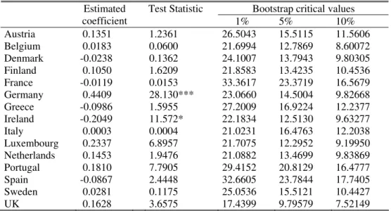
Table 1 shows the results of the causality tests for the EU15 panel for the

period 1960-2006. It is possible to observe that while government revenue positively

causes government spending for Germany and negatively for Ireland, there are more

cases pointing to the spend-and-tax hypothesis: Austria, France, Greece, Italy, Spain,

and Sweden.

[Table1]

We also compared the results (not shown) for two sub-periods, 1960-1985 and

1986-2006. In the first sub-period, causality from revenue to spending occurs in six

countries, while causality from spending to revenue is detected for Greece, Italy and

Portugal. In addition, the tax-and-spend result is obtained for Portugal in the second

sub-period while a negative causality from revenue to spending is found for Italy and

Belgium, which may signal increased concerns regarding fiscal behaviour in the

run-up to EMU. On the other hand, the spend-and-tax result occurs in the second

sub-period for France and Ireland.

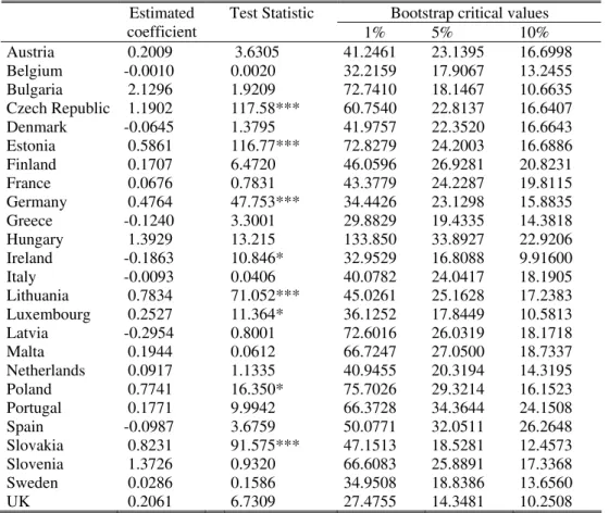
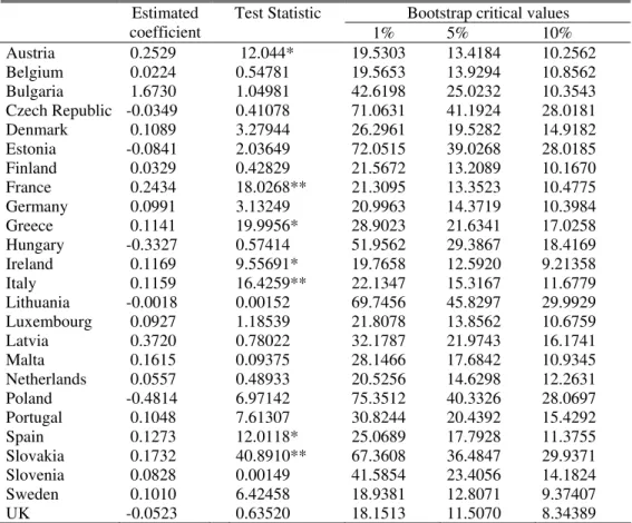
Table 2 reports the results for the EU25 country sample, considering most of

the EU New Member States (NMS). The spend-and-tax result is still found for

Austria, France, Greece, Italy, and Spain, and causality still runs from revenue to

spending in the case of Germany and Luxembourg. On the other hand, the evidence

shows causality from revenue to spending in several EU New Members States: Czech

bi-directional causality between government revenue and spending: Ireland and

Slovakia. Table 3 summarises the causality results.

[Table2]

[Table3]

4. Conclusion

We used a bootstrap panel analysis of causality between government revenue

and spending for the EU, which allows for contemporaneous correlation across

countries and dispenses the need of pre-testing for unit roots. The results support the

so-called spend-and-tax causality for such countries as Italy, France, Spain, Greece,

and Portugal. Tax-and-spend evidence is present notably for Germany, Belgium,

Austria Finland and the UK, and also for several EU New Member States. Some

shifting regarding the direction of the causality patterns can also be detected, after the

2nd half of the 1980s, which may imply adjustments of fiscal behaviour in the run-up

to EMU.

References

Afonso, A. (2005). “Fiscal Sustainability: the Unpleasant European Case”,

FinanzArchiv, 61(1), 19-44.

Afonso, A. and Rault, C. (2007). “What do we really know about fiscal sustainability

in the EU? A panel data diagnostic”, ECB Working Paper n. 820.

Chang, T.; Liu, W., Caudill, S. (2002). “Tax-and-Spend, Spend-and-Tax, or Fiscal

Synchronization: New Evidence for Ten Countries,” Applied Economics, 34(12),

7

Kollias, C., Paleologou, S.-M. (2006). “Fiscal policy in the European Union: Tax and

spend, spend and tax, fiscal synchronisation or institutional separation?” Journal of

Economic Studies, 33(2), 108-120.

Kónya, L. (2006). “Exports and growth: Granger Causality analysis on OECD

countries with a panel approach”, Economic Modelling, 23(6), 978-992.

Payne, J. (2004). “The tax-spend debate: Time series evidence from state budgets”,

Public Choice, 95(3-4), 307-320.

von Furstenberg, G.; Green, R., Jeong, J. (1986). “Tax and spend, or spend and tax?”

Table 1a – Causality from government revenue to spending, EU15 (1960-2006)

Bootstrap critical values Estimated

coefficient

Test Statistic

1% 5% 10%

Austria 0.1351 1.2361 26.5043 15.5115 11.5606

Belgium 0.0183 0.0600 21.6994 12.7869 8.60072

Denmark -0.0238 0.1362 24.1007 13.7943 9.80305

Finland 0.1050 1.6209 21.8583 13.4235 10.4536

France -0.0119 0.0153 33.3617 23.3719 16.5679

Germany 0.4409 28.130*** 23.0660 14.5004 9.82668

Greece -0.0986 1.5955 27.2009 16.9224 12.2377

Ireland -0.2049 11.572* 22.1834 12.5130 9.63277

Italy 0.0003 0.0004 21.0231 16.4763 12.2038

Luxembourg 0.2337 6.8957 21.7075 12.2952 9.19950

Netherlands 0.1453 1.9476 21.0882 13.4699 9.83869

Portugal 0.1810 7.7905 29.4152 20.8129 16.4777

Spain -0.0867 2.4448 32.6605 23.7844 17.7405

Sweden 0.0281 0.1175 25.0536 15.5121 10.4427

UK 0.1628 3.6575 17.4399 9.79579 7.52149

***, **, *: significance at the 1%, 5% and 10% levels, respectively. H0: R does not cause G.

Table 1b – Causality from government spending to revenue, EU15 (1960-2006)

Bootstrap critical values Estimated

coefficient

Test Statistic

1% 5% 10%

Austria 0.2290 8.2731* 22.2499 11.1867 7.9895

Belgium 0.0052 0.0266 18.3643 10.5409 7.73236

Denmark 0.1307 3.9247 23.6322 12.5703 9.37391

Finland 0.0632 1.1145 18.9469 13.1284 9.68753

France 0.3230 25.450*** 19.3738 14.0002 10.7197

Germany 0.1468 5.0713 18.5037 11.7241 8.79791

Greece 0.1043 12.325* 28.6306 16.7483 11.6541

Ireland 0.0988 6.3321 29.5567 12.8465 8.51660

Italy 0.1363 17.783** 27.4934 16.1808 11.8194

Luxembourg 0.0806 0.7435 20.2061 11.3574 8.39400

Netherlands 0.0871 0.9737 19.4031 11.6964 8.71781

Portugal 0.1075 4.9057 26.1445 15.9634 13.1014

Spain 0.1340 10.590* 17.4415 11.5850 8.50721

Sweden 0.1285 8.1168* 15.9548 10.9160 7.76927

UK -0.0434 0.3727 20.3780 10.9510 6.97039

9

Table 2a – Causality from government revenue to spending, EU25 (1960-2006, 1998-2006 for NMS)

Bootstrap critical values Estimated

coefficient

Test Statistic

1% 5% 10%

Austria 0.2009 3.6305 41.2461 23.1395 16.6998

Belgium -0.0010 0.0020 32.2159 17.9067 13.2455

Bulgaria 2.1296 1.9209 72.7410 18.1467 10.6635

Czech Republic 1.1902 117.58*** 60.7540 22.8137 16.6407

Denmark -0.0645 1.3795 41.9757 22.3520 16.6643

Estonia 0.5861 116.77*** 72.8279 24.2003 16.6886

Finland 0.1707 6.4720 46.0596 26.9281 20.8231

France 0.0676 0.7831 43.3779 24.2287 19.8115

Germany 0.4764 47.753*** 34.4426 23.1298 15.8835

Greece -0.1240 3.3001 29.8829 19.4335 14.3818

Hungary 1.3929 13.215 133.850 33.8927 22.9206

Ireland -0.1863 10.846* 32.9529 16.8088 9.91600

Italy -0.0093 0.0406 40.0782 24.0417 18.1905

Lithuania 0.7834 71.052*** 45.0261 25.1628 17.2383

Luxembourg 0.2527 11.364* 36.1252 17.8449 10.5813

Latvia -0.2954 0.8001 72.6016 26.0319 18.1718

Malta 0.1944 0.0612 66.7247 27.0500 18.7337

Netherlands 0.0917 1.1335 40.9455 20.3194 14.3195

Poland 0.7741 16.350* 75.7026 29.3214 16.1523

Portugal 0.1771 9.9942 66.3728 34.3644 24.1508

Spain -0.0987 3.6759 50.0771 32.0511 26.2648

Slovakia 0.8231 91.575*** 47.1513 18.5281 12.4573

Slovenia 1.3726 0.9320 66.6083 25.8891 17.3368

Sweden 0.0286 0.1586 34.9508 18.8386 13.6560

UK 0.2061 6.7309 27.4755 14.3481 10.2508

Table 2b – Causality from government spending to revenue, EU25 (1960-2006, 1998-2006, for NMS)

Bootstrap critical values Estimated

coefficient

Test Statistic

1% 5% 10%

Austria 0.2529 12.044* 19.5303 13.4184 10.2562

Belgium 0.0224 0.54781 19.5653 13.9294 10.8562

Bulgaria 1.6730 1.04981 42.6198 25.0232 10.3543

Czech Republic -0.0349 0.41078 71.0631 41.1924 28.0181

Denmark 0.1089 3.27944 26.2961 19.5282 14.9182

Estonia -0.0841 2.03649 72.0515 39.0268 28.0185

Finland 0.0329 0.42829 21.5672 13.2089 10.1670

France 0.2434 18.0268** 21.3095 13.3523 10.4775

Germany 0.0991 3.13249 20.9963 14.3719 10.3984

Greece 0.1141 19.9956* 28.9023 21.6341 17.0258

Hungary -0.3327 0.57414 51.9562 29.3867 18.4169

Ireland 0.1169 9.55691* 19.7658 12.5920 9.21358

Italy 0.1159 16.4259** 22.1347 15.3167 11.6779

Lithuania -0.0018 0.00152 69.7456 45.8297 29.9929

Luxembourg 0.0927 1.18539 21.8078 13.8562 10.6759

Latvia 0.3720 0.78022 32.1787 21.9743 16.1741

Malta 0.1615 0.09375 28.1466 17.6842 10.9345

Netherlands 0.0557 0.48933 20.5256 14.6298 12.2631

Poland -0.4814 6.97142 75.3512 40.3326 28.0697

Portugal 0.1048 7.61307 30.8244 20.4392 15.4292

Spain 0.1273 12.0118* 25.0689 17.7928 11.3755

Slovakia 0.1732 40.8910** 67.3608 36.4847 29.9371

Slovenia 0.0828 0.00149 41.5854 23.4056 14.1824

Sweden 0.1010 6.42458 18.9381 12.8071 9.37407

UK -0.0523 0.63520 18.1513 11.5070 8.34389

***, **, *: significance at the 1%, 5% and 10% levels, respectively. H0: G does not cause R.

Table 3 – Summary of results

Revenue ⇒Spending

Panel _{∆ R} ⇒_{∆ G}

(tax-and-spend)

∆ R⇒ ∇G

Spending ⇒Revenue (spend-and-tax)

EU15, 1960-2006 Germany Ireland Austria, Italy, France,

Spain, Greece, Sweden EU15, 1960-1985 Belgium, Germany,

Spain, Sweden, Luxembourg, UK

Greece, Italy, Portugal

EU15, 1986-2006 Austria, Finland, Portugal Belgium, Denmark, Italy, Sweden France, Ireland EU25, 1960-2006; NMS, 1998-2006 Czech Republic, Estonia, Lithuania, Poland, Slovakia Germany, Luxembourg

Ireland Slovakia, Austria, France,