Extending the Relational
Algebra with the Mapper
Operator
Paulo Carreira
Ant´onia Lopes
Helena Galhardas
Jo˜ao Pereira
DI–FCUL
TR–05–2
January 2005
Departamento de Inform´atica
Faculdade de Ciˆencias da Universidade de Lisboa
Campo Grande, 1749–016 Lisboa
Portugal
Technical reports are available at http://www.di.fc.ul.pt/tech-reports. The files are stored in PDF, with the report number as filename. Alternatively, reports are available by post from the above address.
Extending the Relational Algebra with the
Mapper Operator
Paulo Carreira1,2 Ant´onia Lopes2
[email protected] [email protected] Helena Galhardas3 Jo˜ao Pereira3
[email protected] [email protected]
1OBLOG Consulting S.A.,
Rua da Barruncheira 4, 2795-477 Carnaxide, Portugal
2Faculty of Sciences of the University of Lisbon,
C6 - Piso 3, 1700 Lisboa, Portugal
3INESC-ID and Technical University of Lisbon,
Avenida Prof. Cavaco Silva, Tagus Park, 2780-990 Porto Salvo, Portugal
January 2005
Abstract
Application scenarios such as legacy data migration,
Extract-Transform-Load (ETL) processes, and data cleaning require the transformation of
input tuples into output tuples. Traditional approaches for implementing these data transformations enclose solutions as Persistent Stored Modules
(PSM) executed by an RDBMS or transformation code using a
commer-cial ETL tool. Neither of these is easily maintainable or optimizable. A third approach consists of combining SQL queries with external code, written in a programming language. However, this solution is not expres-sive enough to specify an important class of data transformations that produce several output tuples for a single input tuple.
In this paper, we propose the data mapper operator as an extension to the relational algebra to address this class of data transformations. Furthermore, we supply a set of algebraic rewriting rules for optimiz-ing expressions that combine standard relational operators with mappers. Finally, experimental results report the benefits brought by some of the proposed semantic optimizations.
1
Introduction
Current data migration applications aim at converting legacy data, stored in sources with a certain schema into target data sources whose schema is dis-tinct and predefined. Organizations often buy new applicational packages (like
SAP [31], for instance) that replace existing ones (e.g., human resources man-agement). This situation leads to the development of data transformation pro-grams that must move data instances from a fixed source schema underlying old applications into a new fixed target schema that supports new applications. The normalization theory underlying the relational model imposes the or-ganization of data according to several relations in order to avoid duplication and inconsistency of information. Therefore, data retrieved from the database is mostly obtained by selecting, joining and unioning relations, as well as by computing aggregates of information. Data transformation applications, how-ever, bring new requirements as their focus is not limited to the idea of selecting information but also involves the production of new data items. Some kinds of data transformations can be defined in terms of relational expressions, if we con-sider relational algebra equipped with a generalized projection operator, where the projection list may include expressions that define the computations to be performed over each selected data (for instance, πID,N AM E←F IRST ||’ ’||LAST).
However, in the context of data migration, there is a considerable amount of data transformations that require one-to-many mappings. In fact, as recognized in [15], an important class of data transformations require the inverse operation of the SQL group by/aggregates primitive [21] that, for each input tuple, has the ability to produce several output tuples.
Up to now, several alternatives have been adopted for implementing one-to-many data mappings: (i) data transformation programs using a programming language, such as C or Java, (ii) an RDBMS proprietary language like Ora-cle PL/SQL; or (iii) data transformation scripts using a commercial ETL tool (e.g., Sagent [30]). However, as we shall analize in Section 1.1, each of these approaches poses a number of drawbacks.
In this paper, we propose an extension to relational algebra to represent one-to-many data transformations. There are two main reasons why we choose to extend relational algebra. First, in the context of ETL programs, many data transformations are in fact naturally expressed as relational algebra queries. Even though the relational algebra is not expressive enough to capture the semantics of one-to-many mappings, we want to make use of the provided ex-pressiveness for the remaining data transformations. Second, we can take ad-vantage of the optimization strategies that are supported by most relational database engines. Our decision of adopting database technology as a basis for data transformation is not completely revolutionary. Several RDBMS, like Mi-crosoft SQL Server, already include additional software packages specific for ETL tasks. However, to the best of our knowledge, none of these extensions is supported by the corresponding theoretical background in terms of existing database theory. Therefore, the capabilities of relational engines, for example, in terms of optimization opportunities are not fully exploited for ETL tasks.
In the remainder of this section, we first present a motivating example to il-lustrate the usefulness of one-to-many data transformations and we then discuss existing alternatives to express and implement this kind of data transformations. In Section 1.3 we highlight the contributions of this paper.
1.1
Motivating example
As already mentioned, there is a considerable amount of data transformations that require one-to-many data mappings. We present a simple example, based
Relation LOANS Relation PAYMENTS
ACCT AM
12 20.00 3456 140.00 901 250.00
ACCTNO AMOUNT SEQNO
0012 20.00 1 3456 100.00 1 3456 40.00 2 0901 100.00 1 0901 100.00 2 0901 50.00 3
Figure 1: (a) On the left, the LOANS relation and, (b) on the right, the PAYMENTS relation.
on a real-world data migration scenario, that has been intentionally simplified for illustration purposes.
Example 1.1: Consider the source relation LOANS[ACCT, AM] (represented in Figure 1) that stores the details of loans requested per account. Suppose LOANS data must be transformed into PAYMENTS[ACCTNO, AMOUNT, SEQNO], the target re-lation, according to the following requirements:
1. In the target relation, all the account numbers are left padded with zeroes. Thus, the attribute ACCTNO is obtained by (left) concatenating zeroes to the value of ACCT.
2. The target system does not support payment amounts greater than 100. The attribute AMOUNT is obtained by breaking down the value of AM into multiple parcels with a maximum value of 100, in such a way that the sum of amounts for the same ACCTNO is equal to the source amount for the same account. Furthermore, the target field SEQNO is a sequence number for the parcel. This sequence number starts at 1 for each sequence of parcels of a given account.
The implementation of data transformations similar to those requested for producing the target relation PAYMENTS of Example 1.1 is challenging, since solutions to the problem involve the dynamic creation of tuples based on the value of attribute AM.
1.2
Discussion of alternative solutions
As referred above, one-to-many data transformations are usually implemented with ad-hoc transformation programs written in a general purpose language; RDBMS proprietary languages like e.g., PL/SQL or, more generally, a set of
Persistent Stored Modules (PSMs) to be executed by an RDBMS; or a data
transformation script using the proprietary programming language of some com-mercial ETL tool. We now detail the drawbacks of each of these alternatives. 1.2.1 General purpose programming language
The use of a general purpose language is hindered by two factors. First, these languages have a procedural nature as opposed to the declarative nature of query
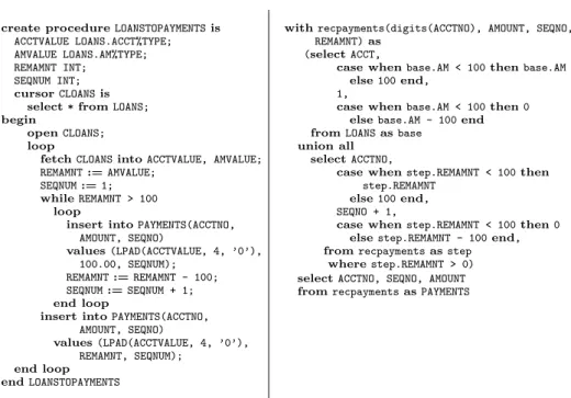
create procedure LOANSTOPAYMENTS is ACCTVALUE LOANS.ACCT%TYPE; AMVALUE LOANS.AM%TYPE; REMAMNT INT; SEQNUM INT; cursor CLOANS is
select * from LOANS; begin
open CLOANS; loop
fetch CLOANS into ACCTVALUE, AMVALUE; REMAMNT := AMVALUE;
SEQNUM := 1; while REMAMNT > 100
loop
insert into PAYMENTS(ACCTNO, AMOUNT, SEQNO) values (LPAD(ACCTVALUE, 4, ’0’), 100.00, SEQNUM); REMAMNT := REMAMNT - 100; SEQNUM := SEQNUM + 1; end loop
insert into PAYMENTS(ACCTNO, AMOUNT, SEQNO)
values (LPAD(ACCTVALUE, 4, ’0’), REMAMNT, SEQNUM);
end loop end LOANSTOPAYMENTS
with recpayments(digits(ACCTNO), AMOUNT, SEQNO, REMAMNT) as
(select ACCT,
case when base.AM < 100 then base.AM else 100 end,
1,
case when base.AM < 100 then 0 else base.AM - 100 end from LOANS as base
union all select ACCTNO,
case when step.REMAMNT < 100 then step.REMAMNT
else 100 end, SEQNO + 1,
case when step.REMAMNT < 100 then 0 else step.REMAMNT - 100 end, from recpayments as step
where step.REMAMNT > 0) select ACCTNO, SEQNO, AMOUNT from recpayments as PAYMENTS
Figure 2: RDBMS implementation of Example 1.1. (a) On the left, an Oracle PL/SQL stored procedure; (b) On the right, an SQL recursive query using IBM DB2 SQL.
languages. This characteristic turns data transformations difficult to understand and maintain. Second, apart from some static optimizations, transformation programs cannot be optimized. If the topology of the data instance changes, answering the query using a different algorithm is only possible after recompiling the code.
1.2.2 RDBMS Persistent Stored Modules
To illustrate the inconvenients of implementing data transformation programs using an RDBMS, we show the implementation of Example 1.1 data transforma-tion using PL/SQL (as presented in Figure 2a) and through an SQL recursive query (on Figure 2b).
The PL/SQL stored procedure that corresponds to Example 1.1 is consti-tuted by two sections: a declarations section and a body section. In the section of declarations, we declare a set of working variables that are used in the pro-cedure body. We also declare the cursor CLOANS that will be used for iterating through the LOANS table. In the body, we start by opening the input cursor. Then, a loop and a fetch statement are used for iterating over it. The loop is broken when the fetch statement fails to retrieve more tuples from CLOANS. The value contained in ACCTVALUE is loaded into the working variable REMAMNT. Then, the value of this variable is decreased in parcels of 100. An inner loop is used to form the parcels based on the value of REMAMNT. A new parcel row is inserted in the target table PAYMENTS for each iteration of the inner loop. The tuple is inserted through an insert into statement that is also responsi-ble for the padding the value of ACCTVALUE with zeroes. When the inner loop
breaks, an insert into statement is issued to insert the parcel that contains the remainder.
The use of PSMs has two inconveniences. First, PSM programs have a num-ber of procedural constructs that are not amenable to optimization. Moreover, there are no elegant solutions for expressing the dynamic creation of instances using PSMs. One needs to resort to intricate loop and insert into statements as shown in Figure 2a, where the relation PAYMENTS is populated through insert into statements. From the description of Example 1.1, we conclude that the logic to compute each of its attributes is distinct. Nevertheless, in the PL/SQL code, the computation of ACCTNO is coupled with the computation of AMOUNT. Furthermore, the logic to calculate ACCTNO is duplicated in the code. This dif-ficults code maintenance and clearly is not easily optimizable.
In the particular case of Example 1.1, the semantics of one-to-many map-pings can be emulated by a recursive query (see [2] for a survey) as the one presented in Figure 2b. Recursion with stratified negation is supported in SQL 1999 [22]. One-to-many mappings can also be implemented using the notion of table functions in SQL 2003 [12]. However, in both cases, complex SQL clauses have to be specified and there is little possibility of optimization.
A recursive query written in SQL 1999 is divided in three sections. The first section is the base of the recursion that creates the initial result set (as presented in Figure 2b. The second section, known as the step, is evaluated recursively on the result set obtained so far. The third section specifies a query responsible for returning the final result set. In the base step, the first parcel of each loan is created and extended with the column REMAMNT whose purpose is to track the remaining amount. Then, at each step we enlarge the set of resulting rows. All rows with REMAMNT are already a valid parcel and are not expanded by recursion. Those rows with REMAMNT > 100 will generate a new row with a new sequence number set to SEQNO + 1 and with remaining amount decreased by 100. Finally, the PAYMENTS table is generated by projecting away the extra REMAMNT column.
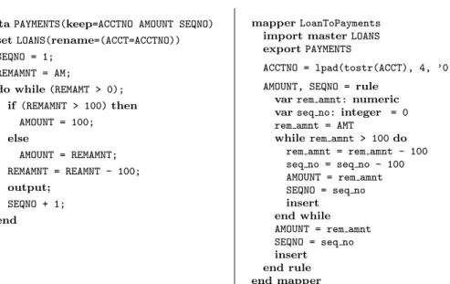
1.2.3 ETL tool proprietary programming languages
We also implemented Example 1.1 using the component of the SAS system [32] which is responsible for data wharehouse construction. The code is shown in Figure 3. In SAS, iterating on the input table LOANS and materializing the results are implicit operations. The assignment of the account number is performed by renaming ACCT as ACCTNO. In the two working variables used for populating each new parcel are declared and initialized. The do while loop is used to produce the output rows. The output values are loaded into the corresponding attributes, and a new parcel is generated through the output statement.
Data Fusion is a data transformation tool that supports a data transforma-tion language named DTL, whose main primitive is the mapper. The input and output relations of a mapper are specified in the header. The body of the map-per is constituted of rules that attempt to isolate as much as possible the way output attributes are obtained from the source relation. Figure 3b presents the specification that implements Example 1.1 using the Data Fusion. The mapping code used to load the target attribute ACCTNO is kept outside the loop. This principle is highly beneficial because we often encounter target tables with tens
data PAYMENTS(keep=ACCTNO AMOUNT SEQNO) set LOANS(rename=(ACCT=ACCTNO)) SEQNO = 1; REMAMNT = AM; do while (REMAMT > 0); if (REMAMNT > 100) then AMOUNT = 100; else AMOUNT = REMAMNT; REMAMNT = REAMNT - 100; output; SEQNO + 1; end mapper LoanToPayments import master LOANS export PAYMENTS
ACCTNO = lpad(tostr(ACCT), 4, ’0’) AMOUNT, SEQNO = rule
var rem amnt: numeric var seq no: integer = 0 rem amnt = AMT
while rem amnt > 100 do rem amnt = rem amnt - 100 seq no = seq no - 100 AMOUNT = rem amnt SEQNO = seq no insert
end while AMOUNT = rem amnt SEQNO = seq no insert
end rule end mapper
Figure 3: Implementation of Example 1.1 using ETL tools that support the dynamic creation of tuples. (a) On the left, the implementation as an SAS Data Step; (b) On the right, the specification in Data Fusion, a data migration tool.
of columns in real-world examples and nesting all rules inside the loop would compromise their readability.
The mapping logic that loads the target attributes AMOUNT and SEQNO is performed through a separate rule. A working variable rem amnt is initialized with the value of AMT and used to partition the total amount into parcels of 100. The dynamic creation of records is achieved by nesting an insert statement into a while loop. Each time an insert is executed, a new value for the target column is associated with the rule. The values produced by each rule are then combined to generate target records.
By comparison with the RDBMS approaches presented in Figure 2, the code for implementing the transformations using ETL tools is more concise. This is dued to the fact that these tools use domain specific languages [41] with built-in support for dynamic creation of records. However, to the best of our knowledge, no other ETL tool, besides SAS and Data Fusion provides native support for this functionality. Some ETL tools (e.g., Sagent [30] and Datastage [3]) do provide an extensive library of predefined functions, but none of them allows expressing the dynamic creation of records. This involves either (i) writing complex proprietary language scripts or (ii) coding external functions. Furthermore, and perhaps most importantly, no ETL tool provides optimization opportunities that depend on the data handled.
1.3
Major contributions
This paper proposes to extend relational algebra with the mapper operator, which significantly increases its expressive power by representing one-to-many data transformations. Informally, a mapper is applied to an input relation and produces an output relation. It iterates over each input tuple and generates
one or more output tuples, by applying a set of domain-specific functions. In this way, it supports the dynamic creation of tuples based on a source tuple contents. This kind of operation appears implicitly in most languages aiming at implementing schema and data transformations but, as far as we know, has never been properly handled as a first-class operator. New optimization opportunities arise when promoting the mapper to a relational operator. In fact, expressions that combine the mapper operator with standard relational algebra operators can be optimized.
The two main contributions of this paper are the following:
• the formalization of a new primitive operator, named data mapper, that
allows expressing one-to-many mappings;
• a set of provably correct algebraic rewriting rules for expressions
involv-ing the mapper operator and relational operators, useful for optimization purposes.
The paper is organized as follows. Some preliminary definitions are provided in Section 2. The formalization of the mapper is presented in Section 3. Section 4 presents the algebraic rewriting rules that enable the optimization of several expressions involving the mapper operator. Practical evidence that shows the advantage of one of these optimizations is presented in Section 5. Finally, related work is summarized in Section 6 and conclusions are presented in Section 7.
2
Preliminaries
We start by introducing the notation we will use throughout the paper, following [4].
A domain D is a set of atomic values. We assume a set D of domains and a set A of names – attribute names – together with a function Dom : A → D that associates attributes to domains. We will also use Dom to denote the natural extension of this function to lists of attribute names: Dom(A1, ..., An) =
Dom(A1) × ... × Dom(An).
A relation schema consists of a name R (the relation name) along with a list
A = A1, ..., An of distinct attribute names. We write R(A1, ..., An), or simply
R(A), and call n the degree of the relation schema. Its domain is defined by Dom(A). A relation instance (or relation, for short) of R(A1, ..., An) is a finite
set r ⊆ Dom(A1) × ... × Dom(An); we write r(A1, ..., An), or simply r(A). Each
element t of r is called a tuple or r-tuple and can be regarded as a function that associates a value of Dom(Ai) with each Ai; we denote this value by t[Ai].
Given a list B = B1, ..., Bk of distinct attributes in A1, ..., An, we denote by
t[B] the tuple ht[B1], ..., t[Bk]i in Dom(B).
We will use the term relational algebra to denote the standard notion as introduced by [10]. The basic operations considered are union, difference and
Cartesian product as well as projection (πX, where X is a list of attributes),
selection (σC, where C is the selection condition) and renaming (ρA→B, where
3
The mapper operator
In this section, we present the definition of the new mapper operator and define other basic concepts. We assume two fixed relation schemas S(X1, ..., Xn) and
T (Y1, ..., Ym). We refer to S and T as the source and the target relation schemas,
respectively.
A mapper is a unary operator µF that takes a relation instance of the source
relation schema as input and produces a relation instance of the target relation schema as output. The mapper operator is parameterized by a set F of special functions, which we designate as mapper functions.
Roughly speaking, each mapper function allows one to express a part of the envisaged data transformation, focused on one or more attributes of the target schema. Although the idea is to apply mapper functions to tuples of a source relation instance, it may happen that some of the attributes of the source schema are irrelevant for the envisaged data transformation. The explicit identification of the attributes that are considered relevant is then an important part of a mapper function. Mapper functions are formally defined as follows.
Definition 3.1: Let A be a non-empty list of distinct attributes in Y1, ..., Ym.
An A−mapper function consists of a non-empty list of distinct attributes B in X1, ..., Xn and a computable function fA:Dom(B)→P(Dom(A)).
Let t be tuple of a relation instance of the source schema. We define fA(t)
to be the application of the underlying function fAto the tuple t, i.e., fA(t[B]).
In this way, mapper functions describe how a specific part of the target data can be obtained from the source data. The intuition is that each mapper function establishes how the values of a group of attributes of the target schema can be obtained from the attributes of the source schema. The key point is that, when applied to a tuple, a mapper function produces a set of values, rather than a single value.
We shall freely use fAto denote both the mapper function and the function
itself, omitting the list B whenever its definition is clear from the context, and this shall not cause confusion. We shall also use Dom(fA) to refer to it. This list
should be regarded as the list of the source attributes declared to be relevant for the part of the data transformation encoded by the mapper function. Notice, however, that even if fA is a constant function, fA may be defined as being
dependent on all the attributes of the source schema. The relevance of the explicit identification of these attributes will be clarified in Section 4 when we present the algebraic optimization rules for projections.
Certain classes of mapper functions enjoy properties that enable the op-timizations of algebraic expressions containing mappers (see also Section 4). Mapper functions can be classified according to (i) the number of output tu-ples they can produce, or according to (ii) the number of output attributes. Mapper functions that produce singleton sets, i.e., ∀(t ∈ Dom(X)) |fY(t)| = 1
are designated single-valued mapper functions. In contrast, mapper functions that produce multiple elements are said to be multi-valued mapper functions. Concerning the number of output attributes, mapper functions with one out-put attribute are called single-attributed, whereas functions with many outout-put attributes are called multi-attributed.
We designate by identity mapper functions the single-valued functions de-fined as fA: Dom(B) → P(Dom(A)) s.t. fA(t) = {t}. Notice that this is only
possible when Dom(B) = Dom(A).
As mentioned before, a mapper operator is parametrized by a set of mapper functions. This set is proper for transforming the data from the source to the target schemas if it specifies, in a unique way, how the values of every attribute of the target schema are produced.
Definition 3.2: A set F = {fA1, ..., fAk} of mapper functions is said to be proper (for transforming the data of S into T) iff every attribute Yi of the target
relation schema is an element of exactly one of the Aj lists, for 1 ≤ j ≤ k.
The mapper operator µF puts together the data transformations of the input
relation defined by the mapper functions in F . Given a tuple s of the input relation, µF(s) consists of the tuples t of Dom(Y ) that, to each list of attributes
Ai, associate a list of values in fAi(s). Formally, the mapper operator is defined as follows.
Definition 3.3: Given a relation s(X) and a proper set of mapper functions
F = {fA1, ..., fAk}, the mapper of s with respect to F , denoted by µF(s), is the
relation instance of the target relation schema defined by
µF(s)def= {t ∈ Dom(Y ) | ∃u ∈ s s.t. t[Ai] ∈ fAi(u), ∀1 ≤ i ≤ k} We designate the relation s as the input (or source) relation of the mapper, and the relation t is the output (or target) relation of the mapper. In order to illustrate this new operator, we revisit Example 1.1.
Example 3.1: The requirements presented in Example 1.1 can be described by the mapper µacct,amt, where acct is an ACCT-mapper function that returns
a singleton with the account number ACCT properly left padded with zeroes and amt is the [AMOUNT,SEQNO]-mapper function s.t., amt(am) is given by
{(100, i) | 1 ≤ i ≤ (am/100)} ∪ {(am%100, (am/100) + 1) | am%100 6= 0} where we have used / and % to represent the integer division and modulus op-erations, respectively.
For instance, if t is the source tuple (901, 250.00), the result of evaluating amt(t) is the set {(100, 1), (100, 2), (50, 3)}. Given a source relation s including t, the result of the expression µacct,amt(s) is a relation that contains the set of
tuples {h’0901’, 100, 1i, h’0901’, 100, 2i, h’0901’, 50, 3i}.
In order to illustrate the full expressive power of mappers, we present an example of selective transformation of data.
Example 3.2: Consider the conversion of yearly data into quarterly data. Let
EMPDATA[ESSN, ECAT, EYRSAL] be the source relation that contains yearly salary information about employees. Suppose we need to generate a target relation with schema EMPSAL[ENUM, QTNUM, QTSAL], which maintains the quarterly salary for the employees with long-term contracts. In the source schema, we assume that the attribute EYRSAL maintains the yearly net salary. Furthermore, we
consider that the attribute ECAT holds the employee category and that code ’S’ specifies a short-term contract whereas ’L’ specifies a long-term contract.
This transformation can be specified through the mapper µempnum,sal where
empnum is a ENUM-mapper function that makes up new employee numbers (i.e., a Skolem function [20]), and sal the [QTNUM, QTSAL]-mapper function
salQTNUM, QTSAL(ecat, eyrsal)
that generates quarterly salary data, defined as: sal(ecat, eyrsal) = ½ {(i,eyrsal 4 ) | 1 ≤ i ≤ 4} if ecat = ’L’ ∅ if ecat = ’S’
3.1
Properties of Mappers
We start to notice that, in some situations, the mapper operator admits a more intuitive definition in terms of the Cartesian product of the sets of tuples obtained by applying the underlying mapper functions to each tuple of the input relation. More concretely, the following proposition holds.
Proposition 1: Given a relation s(X) and a proper set of mapper functions
F = {fA1, ..., fAk} s.t. A1· ... · Ak= Y , µF(s) = [ u∈s fA1(u) × ... × fAk(u). Proof
µF(s) = {t ∈ Dom(Y ) | ∃u ∈ s s.t. t[Ai] ∈ fAi(u), ∀1 ≤ i ≤ k}
= [
u∈s
{t ∈ Dom(Y ) | t[Ai] ∈ fAi(u), ∀1 ≤ i ≤ k}
= [
u∈s
fA1(u) × ... × fAk(u)
u t
This alternative way of defining µF(s) is also important because of its
oper-ational flavor, equipping the mapper operator with a tuple-at-a-time semantics. When integrating the mapper operator with existing query execution processors, this property plays an important role because it means the mapper operator ad-mits physical execution algorithms that favor pipelined execution [17].
The task of devising an algorithm that computes data transformation through mappers becomes straightforward: if every underlying mapper function only in-volves adjacent attributes of the target relation schema and in the same order (i.e., A1· ... · Ak = Y ), then it is just to compute the Cartesian product as stated
by the proposition; in the other situations, after calculating the Cartesian prod-uct, it is necessary to exchange the elements of each tuple so they become in the correct order. Obviously, this algorithm relies on the computability of the underlying mapper functions and builds on concrete algorithms for computing them.
Furthermore, the fact that the calculation of µF(s) can be carried out tuple
Proposition 2 : The mapper operator is monotonic, i.e., for every pair of
relations s1(X) and s2(X) s.t. s1⊆ s2, µF(s1) ⊆ µF(s2).
Proof
µF(s1) = {t ∈ Dom(Y ) | ∃u ∈ s1 s.t. t[Ai] ∈ fAi(u), ∀1 ≤ i ≤ k} by hypothesis s1⊆ s2
⊆ {t ∈ Dom(Y ) | ∃u ∈ s2 s.t. t[Ai] ∈ fAi(u), ∀1 ≤ i ≤ k} = µF(s2)
u t
Mapper operators whose mapper functions are all single-valued admit an equivalent mapper with only one mapper function.
Proposition 3 : Given a set F = {fA1, ..., fAk} of single-valued mapper
functions proper for transforming S(X) into T (Y ). For every mapper µF,
there exists an equivalent mapper with only one Y −mapper function gY, s.t.,
µF = µ{gY}.
Proof It suffices to show how to obtain gY. Consider the mapper function
gY[Yi] = fAi, for every 1 ≤ i ≤ k. The result is obtained by juxtaposition of
the values produced by each function fAi∈ F . ut
3.2
Expressive power of mappers
Concerning the expressive power of the mapper operator, two important ques-tions are addressed. First, we compare the expressive power of relational algebra (RA) with its extension by the set of mapper operators, henceforth designated as M-relational algebra or simply MRA. Second, we investigate which standard relational operators can be simulated by a mapper operator.
It is not difficult to recognize that MRA is more expressive than standard RA. It is obvious that part of the expressive power of mapper operators comes from the fact that they are allowed to use arbitrary computable functions. In fact, the class of mapper operators of the form µ{f }, where f is a single-valued
function, is computationally complete. This implies that MRA is computational complete and, hence, MRA is not a query language like standard RA.
The question that naturally arises is if MRA is more expressive than the relational algebra with a generalized projection operator πLwhere the projection
list L has elements of the form Yi ← f (A), where A is a list of attributes in
X1, ..., Xn and f is a computable function.
With generalized projection, it becomes possible to define arbitrary compu-tations to derive the values of new attributes. Still, there are MRA-expressions whose effect is not expressible in RA, even when equipped with the general-ized projection operator. We shall use RA-gp to designate the extension of RA extended with generalized projection.
The additional expressive power results from the fact that mapper operators use functions that map values into sets of values and, thus, are able to produce a set of tuples from a single tuple. For some multi-valued functions, the number of tuples that are produced depends on the specific data values of the source tuples and does not even admit an upper-bound.
Consider for instance a database schema with relation schemas S(NUM) and T(NUM, IND), s.t. the domain of NUM and IND is the set of natural numbers. Let
s be a relation with schema S. The cardinality of the expression µ{f }(s), where
f is an [NUM,IND]-mapper function s.t. f (n) = {hn, ii : 1 ≤ i ≤ n}, does not
(strictly) depend on the cardinality of s. Instead, it depends on the values of the concrete s−tuples. For instance, if s is a relation with a single tuple {hxi}, the cardinality of µ{f }(s) depends on the value of x and does not have an upper
bound.
This situation is particularly interesting because it cannot happen in RA-gp. Proposition 4: For every expression E of the relational algebra RA-gp, the
cardinality of the set of tuples denoted by E admits an upper bound defined simply in terms of the cardinality of the atomic sub-expressions of E.
Proof This can be proved in a straightforward way by structural induction in the structure of relational algebra expressions. Given a relational algebra expression E, we denote by |E| the cardinality of E. For every non-atomic expression we have: |E1∪ E2| ≤ |E1| + |E2|; |E1− E2| ≤ |E1|; |E1× E1| ≤
|E1| × |E2|; |πL(E)| ≤ |E|; |σC(E)| ≤ |E|. ut
Hence, it follows that:
Proposition 5: There are expressions of the M-relational algebra that are not
expressible by the relational algebra RA-gp on the same database schema.
Another aspect of the expressive power of mappers, that is interesting to address, concerns the ability of mappers for simulating other relational opera-tors. In fact, we will show that renaming, projection and selection operators can be seen as special cases of mappers. That is to say, there exist three classes of mappers that are equivalent, respectively, to renaming, projection and selec-tion. From this we can conclude that the restriction of MRA to the operators mapper, union, difference and Cartesian product is as expressive as MRA.
Renaming and projection can be obtained through mapper operators over identity mapper functions.
Rule 1: Let S(X1, ..., Xn) and T (Y1, ..., Ym) be two relation schemas s.t. Y is
a sublist of X and let s be a relation instance of S(X). The term πY1,...,Ym(s)
is equivalent to µF(s) where F = {fY1, ..., fYm} and, for every 1 ≤ i ≤ m, fYi
is the identity function over Dom(Yi).
Proof
πY1,...,Ym(s) = {t[Y1, ..., Ym] | t ∈ s}
= {t ∈ Dom(Y ) | ∃u ∈ s s.t. u[Yi] = t[Yi], ∀1 ≤ i ≤ m}
= {t ∈ Dom(Y ) | ∃u ∈ s s.t. u[Yi] ∈ {t[Yi]}, ∀1 ≤ i ≤ m}
because fYi is the identity on Dom(Yi)
= {t ∈ Dom(Y ) | ∃u ∈ s s.t. u[Xi] ∈ fYi(t), ∀1 ≤ i ≤ m} = µfY1,...,fYm(s)
u t
Rule 2: Let S(X1, ..., Xn) and T (Y1, ..., Yn) be two relation schemas, such that,
Dom(X) = Dom(Y ) and let s be a relation instance of S(X). Then, the term
ρX1,...,Xn→Y1,...,Yn(s) is equivalent to µF(s) where F = {fY1, ..., fYn} and, for
every 1 ≤ i ≤ n, fYi is the identity mapper function over Dom(Yi). Proof
ρX1,...,Xn→Y1,...,Yn(s)
= {t ∈ Dom(Y ) | ∃u ∈ s s.t. u[Xi] = t[Yi], ∀1 ≤ i ≤ n}
= {t ∈ Dom(Y ) | ∃u ∈ s s.t. u[Xi] ∈ {t[Yi]}, ∀1 ≤ i ≤ n}
because fYi is the identity on Dom(Yi)
= {t ∈ Dom(Y ) | ∃u ∈ s s.t. u[Xi] ∈ fYi(t), ∀1 ≤ i ≤ n} = µfY1,...,fYn(s)
u t
Since mapper functions may map input tuples into empty sets (i.e., no output values are created), they may act as filtering conditions which enable the mapper to behave not only as a tuple producer but also as a filter.
Rule 3: Let S(X1, ..., Xn) be a relation schema, C a condition over the
at-tributes of this schema and s(X) a relation. There exists a set F of proper mapper functions for transforming S(X) into S(X) s.t. the term σC(s) is
equiv-alent to µF(s).
Proof It suffices to show how F can be constructed from C and prove the equivalence of σCand µF. Let F be {fX1, ..., fXn} where each mapper function
fXi is defined by the function with signature Dom(X) → P(Dom(Xi)) s.t.
fXi(t) = (
{t[Xi]} if C(t)
∅ if ¬C(t)
We have,
µF(s) = {t ∈ Dom(X) | ∃u ∈ s s.t. t[Xi] ∈ fXi(u), ∀1 ≤ i ≤ n} by the definition of fXi
= {t ∈ Dom(X) | ∃u ∈ s s.t. t[Xi] ∈ {u[Xi]} and C(u), ∀1 ≤ i ≤ n}
= {t ∈ Dom(X) | ∃u ∈ s s.t. t[Xi] = u[Xi] and C(u), ∀1 ≤ i ≤ n}
= {t ∈ Dom(X) | ∃u ∈ s s.t. t = u and C(u)} = {t ∈ Dom(X) | t ∈ s and C(t)}
= σC(s)
u t
4
Algebraic optimization rules
Algebraic rewriting rules are equations that specify the equivalence of two alge-braic terms. Through algealge-braic rewriting rules, queries presented as relational
expressions can be transformed into equivalent ones that are more efficient to evaluate [38]. In this section we present a set of algebraic rewriting rules that en-able algebraic optimizations of relational expressions extended with the mapper operator.
One commonly used strategy in query rewriting aims at reducing execution cost by transforming relational expressions into equivalent ones that, from an operational point of view, minimize the amount of information passed from one operator to the next operator. Most algebraic rewriting rules for query optimization proposed in literature fall into one of the following two categories. The first category consists of rules for pushing selections. These rules attempt to reduce the cardinality of the source relations by forcing selections to be evaluated as early as possible. The second category consists of rules for pushing
projections, which are used to avoid propagating attributes that are not used
by subsequent operators. In the following, we adapt these classes of algebraic rewriting rules to the mapper operator.
4.1
Pushing selections to mapper functions
When applying a selection to a mapper we can take advantage of the map-per semantics to introduce an important optimization. Given a selection σCAi
applied to a mapper µfA1,...,fAk, this optimization consists of pushing the
selec-tion σCAi, where CAiis a condition on the attributes produced by some mapper function fAi, directly to the output of the mapper function. Rule 4 formalizes this notion.
Rule 4 : Let F = {fA1, ..., fAk} be a set of multi-valued mapper functions,
proper for transforming S(X) into T (Y ). Consider a condition CAi dependent
on a list of attributes Ai such that fAi ∈ F . Then,
σCAi(µF(s)) = µF \{fAi}∪{σCAi◦fAi}(s)
where (σCAi ◦ fAi)(t) = {fAi(t) | CAi(t)}. Proof
σCAi(µF(s)) = {t ∈ Dom(Y ) | t ∈ µF(s) and CAi(t[Ai])} = {t ∈ Dom(Y ) | ∃u ∈ s s.t. t[Aj] ∈ fAj(u),
and CAi(t[Ai]), ∀1 ≤ j ≤ k}
= {t ∈ Dom(Y ) | ∃u ∈ s s.t. (t[Aj] ∈ fAj(u) if j 6= i) or (t[Aj] ∈ {v ∈ fAj(u) | CAj(u)} if j = i), ∀1 ≤ j ≤ k} = {t ∈ Dom(Y ) | ∃u ∈ s s.t. (t[Aj] ∈ fAj(u) if j 6= i) or
(t[Aj] ∈ σCAi(fAj(u)) if j = i), ∀1 ≤ j ≤ k} = µF \{fAi}∪{σCAi◦fAi}(s)
u t
The benefits of Rule 4 can be better understood at the light of the alternative definition for the mapper semantics in terms of a Cartesian product presented in Section 3.1. Intuitively, it follows from Proposition 1, that the Cartesian product
expansion generated by fA1(u) × ... × fAk(u) can produce duplicate values for some set of attributes Ai, 1 ≤ i ≤ k. Hence, by pushing the condition CAi to the mapper function fAi, the condition will be evaluated fewer times. This is especially important if we are speaking of expensive predicates, like those involving expensive functions or sub-queries (e.g., evaluating the SQL exists operator). See, e.g., [19] for details.
Furthermore, note that when CAi(t) does not hold, the function σCAi(fAi)(t) returns the empty set. When some mapper function fAi returns an empty set, the Cartesian product of the results of all mapper function will also be an empty set. Hence, we may skip the evaluation of all mapper functions fAj, such that j 6= i. Physical execution algorithms for the mapper operator can take advantage of this optimization by evaluating fAi before any other mapper function1. Even in situations where neither expensive functions nor expensive
predicates are present, this optimization can be employed as it alleviates the average cost of the Cartesian product, which depends on the cardinalities of the sets of values produced by the mapper functions.
4.2
Pushing selections through mappers
Another important optimization consists of pushing the selection through the mapper operator. To that aim, we need to rewrite the selection condition. For example, consider the expression σY >4(µX2→Y(s)). The selection condition is
expressed in terms of attributes of the mapper output relation. In order to push σY >4 over the mapper µX2→Y, we need to rewrite it according to the
attributes of the mapper input relation. In this simple case, the expression
µX2→Y(σX<−2 ∨X>2(s)) is equivalent to the original one. However, this kind
of rewriting cannot be fully automated. An alternative way of rewriting expres-sions of the form σC(µF(s)) consists of replacing the attributes in the condition
with the mapper functions that compute them.
Suppose that, in the selection condition C, attribute A is produced by the mapper function fA. By replacing the attribute A with the mapper function fA
in condition C we obtain an equivalent condition. For instance, consider C to be the condition A < 10 in the expression σA<10(µfA(s)). Attribute A can be expanded with the corresponding mapper function to obtain µfA(σfA<10(s)).
In order to formalize this notion, we first need to introduce some notation. Let F = {fA1, ..., fAk} be a set of mapper functions proper for transforming
S(X) into T (Y ). The function resulting from the restriction of fAi to an at-tribute Yj ∈ Ai is denoted by fAi ↓ Yj. Moreover, given an attribute Yj ∈ Y ,
F ↓ Yj represents the function fAi ↓ Yj s.t. Yj ∈ Ai. Note that, because F is a proper set of mapper functions, the function F ↓ Yj exists and is unique.
Rule 5 : Let F = {fA1, ..., fAk} be a set of single-valued mapper functions,
proper for transforming S(X) into T (Y ). Let B = B1 · ... · Bk be a list of
attributes in Y and s a relation instance of S(X). Then, σCB(µF(s)) = µF(σC[B1,...,Bk←F ↓B1,...,F ↓Bk](s))
1The reader may have remarked that this optimization can be generalized to first evaluate
those functions with higher probability of yielding an empty set. This issue is fundamentally the same as the problem of optimal predicate ordering addressed in [19].
where CB means that C depends on the attributes of B, and the condition
that results from replacing every occurrence of each Bi by Ei is represented
as C[B1, ..., Bn ← E1, ..., En].
Proof In order to proove Rule 5 we proceed in two steps. We start by expand-ing both expressions into their correspondexpand-ing sets of tuples Then we establish the equivalence of these sets. So, on the one hand we have that,
σCB(µF(s)) = {t ∈ Dom(Y ) | t ∈ µF(s) and CB(t)} = {t ∈ Dom(Y ) | ∃u ∈ s s.t. t[Ai] ∈ fAi(u),
and CB(t), ∀1 ≤ i ≤ k}
(1)
On the other hand we have that,
µF(σC[B1,...,Bk←F ↓B1,...,F ↓Bk](s))
= {t ∈ Dom(Y ) | ∃u ∈ σC[B1,...,Bk←F ↓B1,...,F ↓Bk] s.t.
t[Ai] ∈ fAi(u), ∀1 ≤ i ≤ k}
=©t ∈ Dom(Y ) | ∃u ∈ {v ∈ Dom(X) | v ∈ s and
C[B1, ..., Bk← F ↓ B1, ..., F ↓ Bk](v)} s.t. t[Ai] ∈ fAi(u), ∀1 ≤ i ≤ k ª = {t ∈ Dom(Y ) | ∃u ∈ s s.t. t[Ai] ∈ fAi(u)
and C[B1, ..., Bk← F ↓ B1, ..., F ↓ Bk](u), ∀1 ≤ i ≤ k}
(2) It now remains to be proven that if fAi(u) = t[Ai], ∀1 ≤ i ≤ n then
C[B1, ..., Bk ← F ↓ B1, ..., F ↓ Bk](u) iff CB(t)
This trivially follows by the defintion of F ↓ Bi and the fact that all functions
are single-valued. ut
This rule replaces each attribute Bi in the condition C by the expression
that describes how its values are obtained. It can be argued that implementing this rewriting rule adds an extra computation, which is caused by the evaluation of the mapper function both in the mapper and in the selection condition. This extra cost can be worthwhile. Consider the case of a selection condition CBi involving an attribute Bi generated by a mapper with two mapper functions:
a cheap mapper function fBi and some expensive mapper function gBj. De-pending on the number of tuples filtered by the condition C[Bi← fBi], the cost of evaluating fBi twice may be insignificant when compared with the cost of producing a tuple (that ultimately will be discarded by the selection condition
CBi) evaluating the function gBj.
Often, the attributes used in the condition of a selection are generated ei-ther by (i) identity mapper functions or (ii) constant mapper functions. In the former case, we may push the condition by renaming its attributes. For exam-ple, by renaming the attributes of the condition A < B we may rewrite the expression σA<B(µX→A,Y →B,fC(s)) as µX→A,Y →B,fC(σX<Y(s)). In the later case, we can replace the attributes of the condition C with the constants of the constant mapper functions and produce an equivalent condition. For exam-ple, in σA<B(µX→A,10→B,fC(s)), the attribute B was replaced by the constant
10 to obtain the equivalent expression µX→A,10→B,fC(σX<10(s)). With respect to implementation, this condition: (i) might be faster to evaluate2, and (ii)
may reduce drastically the number of input tuples that has to handeled by the mapper operator.
4.3
Pushing projections
A projection applied to a mapper is an expression of the form πZ(µF(s)). If
F = {fA1, ..., fAk} is a set of mapper functions, proper for transforming S(X) into T (Y ), then an attribute Yiof Y such that Yi6∈ Z, (i.e., that is not projected
by πZ) is said to be projected-away. Attributes that are projected-away suggest
an optimization. Since they are not required for subsequent operations, the mapper functions that generate them do not need to be evaluated. Hence they can, in some situations, be forgotten. More concretely, a mapper function can be forgotten if the attributes that it generates are projected-away. Rule 6 makes this idea precise.
Rule 6 : Let F = {fA1, ..., fAk} be a set of mapper functions, proper for
transforming S(X) into T (Y ). Let Z and Z0 be lists of attributes in Y and
let s be a relation instance of S(X). Then, πZ(µF(s)) = πZ(µF0(s)), where
F0= {f
Ai∈ F | Ai contains at least one attribute in Z}.
Proof We will write “at least one attribute of Ai is in the list Z” in symbols
as Ai∩ Z 6= ∅. Thus,
πZ(µF(s)) = {t[Z] | t ∈ Dom(Y ) and t ∈ µF(s)}
= {t[Z] | t ∈ Dom(Y ) and ∃u ∈ s s.t. t[Ai] ∈ fAi(u), ∀fAi∈ F } since only those attributes of Ai
that are in Z are projected
= {t[Z] | t ∈ Dom(Y ) and ∃u ∈ s s.t. t[Ai] ∈ fAi(u) and Ai∩ Z 6= ∅, ∀fAi ∈ F }
by hypothesis, Ai∩ Z 6= ∅ ⇔ fAi ∈ F
0
= {t[Z] | t ∈ Dom(Y ) and ∃u ∈ s s.t. t[Ai] ∈ fAi(u), ∀fAi ∈ F
0}
= πZ(µF0(s))
u t
Example 4.1: Consider the mapper µacct,amt defined in Example 3.1. The
expression πAMOUNT(µacct,amt(LOANS)) is equivalent to πAMOUNT(µamt(LOANS)). The
acct mapper function is forgotten because the ACCOUNT attribute was projected-away. Conversely, neither of the mapper functions can be forgotten in the ex-pression πACCTNO, SEQNO(µacct,amt(LOANS)).
Concerning Rule 6, it should be noted that if Z = A1·...·Ak(i.e, all attributes
are projected), then F0= F (i.e., no mapper function can be forgotten).
Another important observation is that attributes that are not used as input of any mapper function need not be retrieved from the mapper input relation. 2Comparing with constants is, in principle, faster than comparing with memory locations
Thus, we may introduce a projection that retrieves only those attributes that are relevant for the functions in F0.
Rule 7 : Let F = {fA1, ..., fAk} be a set of mapper functions, proper for
transforming S(X) into T (Y ). Let s be a relation instance of S(X). Then, µF(s) = µF(πN(s)), where N is a list of attributes in X, that only includes the
attributes in Dom(fAi), for every mapper function fAi in F . Proof
µF(s) = {t ∈ Dom(Y ) | ∃u ∈ s s.t. t[Ai] ∈ fAi(u), ∀1 ≤ i ≤ k} by the definition of mapper function,
fAi(u) = fAi(u[B]) = fAi(u[N ])
= {t ∈ Dom(Y ) | ∃u ∈ s s.t. t[Ai] ∈ fAi(u[N ]), ∀1 ≤ i ≤ k} = {t ∈ Dom(Y ) | ∃u ∈ πN(s) s.t. t[Ai] ∈ fAi(u), ∀1 ≤ i ≤ k} = µF(πN(s))
u t
Example 4.2: Consider the relation LOANS[ACCT, AM] of Example 1.1. The attribute AM is an input attribute of the mapper function amt defined in Example 3.1. Thus, the expression µamt(LOANS) as equivalent to µamt(πAM(LOANS)).
4.4
Mappers and other binary operators
Unary operators of relational algebra enjoy useful distribution laws over binary operators. The mapper operator is a unary operator and it allows the following straightforward equivalency to be established.
Rule 8: Let F = {fA1, ..., fAk} be a set of mapper functions, proper for
trans-forming S(X) into T (Y ). Let r and s be relation instances with schema S(X). Then, µF(r ∪ s) = µF(r) ∪ µF(s)
Proof
µF(r ∪ s) = {t ∈ Dom(Y ) | ∃u ∈ (r ∪ s) s.t. t[Ai] ∈ fAi(u), ∀1 ≤ i ≤ k} = {t ∈ Dom(Y ) | ∃u ∈ s s.t. t[Ai] ∈ fAi(u) or ∃v ∈ s s.t.
t[Ai] ∈ fAi(v), ∀1 ≤ i ≤ k} = µF(r) ∪ µF(s)
u t
However, the mapper operator does not distribute over intersection and dif-ference. Another important binary operation is the join, represented as ./C(see
e.g., [37] or [18]). Join operators can be obtained as a combination of a selection with a Cartesian product3 [25]. Concretely, r ./
C s = σC(r × s). Using this
3To be precise, the renaming operator should also be employed when the schemas of r and
s share attributes. We assume disjointness of the schemas for simplicty of presentation. This
equivalence, we note that the mapper operator can be distributed over the join in two steps. We start by pushing the mapper over the selection σC and then
we distribute the mapper over the Cartesian product r × s. For the first step, Rule 5 can be used. However, the second step is hindered by the fact that the set F appropriate for transforming data with the relation schema of r × s does not necessarily contain sets FR and FS for transforming data with the relation
schema of r and s. However, if we can partition F into two disjoint subsets FR
and FS, then the equivalence µF(s × r) = µFS(s) × µFR(r) holds. We formalize this notion in Rule 9.
Rule 9: Let F = {fA1, ..., fAk} be a set of mapper functions proper for
trans-forming SR(X, Y ) into T (Z). Let s and r be relation instances with schemas S(X) and R(Y ) respectively. If there exist ZR and ZS, such that, ZR· ZS = Z,
and two disjoint subsets FR ⊆ F and FS ⊆ F of mapper functions, proper
for transforming, respectively, S(X) into TR(ZR) and R(Y ) into TS(ZS) then
µF(s × r) = µFS(s) × µFR(r). Proof
µF(r × s) = {t ∈ Dom(Z) | ∃u ∈ (r × s) s.t. t[Ak] ∈ fAk(u), ∀fAk∈ F } = {t ∈ Dom(Z) | ∃u ∈ (r × s) s.t. t[Ai] ∈ fAi(u), ∀fAi∈ FR
and t[Aj] ∈ fAj(u), ∀fAj ∈ FS}
since for every fAi∈ FS, Dom(fAi) is in X, and for every fAj ∈ FR, Dom(fAj) is in Y ,
=©t ∈ Dom(Z) | ∃u ∈ (r × s) s.t. ¡t[Ai] ∈ fAi(u[X]), ∀fAi ∈ FR and t[Aj] ∈ fAj(u[Y ]), ∀fAj ∈ FS
¢ª
because {u | u ∈ r × s} = {u | u[R] ∈ r and u[S] ∈ s}, = {t ∈ Dom(Z) | ∃v ∈ r s.t. t[Ai] ∈ fAi(v), ∀fAi ∈ FR and ∃w ∈ s s.t. t[Aj] ∈ fAj(w), ∀fAj ∈ FS} = µFR(r) × µFS(s) u t
5
Practical Validation
In order to validate the optimizations proposed in Section 4.1, we have im-plemented the mapper operator and conducted a number of experiments con-trasting MRA expressions with their optimized equivalent expressions. Our experiments focus on Rule 4, which entirely takes advantage of the mapper operator semantics. Moreover, this rule seems the most promissing in terms of optimization improvements because it exploits savings on the Cartesian product operations.
Our observations show that the proposed algebraic rewriting introduces sub-stancial performance improvements for many interesting cases. Furthermore, we identify relevant factors, like the predicate selectivity and mapper function
fanout, that influence the gain obtained when applying the proposed
5.1
Experimental setup
An implementation of the mapper operator was developed on top of the XXL li-brary4[40, 39], which provides database query processing functionalities through
a set of relational operators. The physical execution algorithms of the relational operators featured by XXL implement the iterator abstraction [17] as found in the Volcano query execution engine [16]. Many modern RDBMS (like Sybase and Microsoft SQL Server) are also based on Volcano. The XXL library is im-plemented in Java5, includes a rule-based optimizer and provides support for
different index-structures, I/O buffering and low level disk accesses.
We conducted our experiments on a standard PC with an Intel Pentium IV processor at 1.9Ghz, 512MB of RAM, Linux kernel version 2.4.2 with ext3 file system and Sun’s JRE 1.4.2. We used stopwatch objects implemented with the Java time utility classes6for performing measurements.
We measured total work, i.e., the sum of the time taken to read the input tuples, to compute the output tuples, and to materialize them. To ascertain that the diferences in performance were caused by improvements brought by an optimized expression over the original, we verified that the amount of I/O performed on both expressions was the same.
5.2
Experiments
In this section, we describe four experiments to analyze the impact of the predi-cate selectivity factor [33], the function fanout factor [6], and the input relation size on the gain obtained with the optimized expression. Besides the cost of evaluating the mapper functions, these three factors are the most relevant fac-tors that influence the cost of the mappper. We do not consider the cost of function evaluation since our optimization, as presented, is unable to improve it.
A mapper function may produce a set of values for each input tuple. Simi-larly to [6], we designate as fanout the average cardinality of the output values produced by a mapper function for each input tuple.
The first experiment we performed, presented in Section 5.2.1, is based on a real world scenario. We aimed at measuring the improvement of total work when optimizing the original expression. Three other experiments were performed, focusing separately on each of the above-mentioned factors. The influence of predicate selectivity, the impact of function fanout and input relation size are analyzed, in Sections 5.2.2, 5.2.3 and 5.2.4, respectively.
These three experiments use a mapper µf1,f2,f3,f4 where, unless otherwise
stated, each mapper function has a fanout factor of 2.0. For the sake of accuracy, we apply predicates that guarantee predefined selectivity values7. Likewise, we
employ functions specifically designed to guarantee predefined fanout factors when we need to vary the fanout of a function.
4One of the main motivations for choosing XXL is the fact that all the packages are fully
documented and publicly available under GNU LGPL[14], which allowed us to quickly test and deploy our ideas.
5Other well-known RDBMS engines like, e.g., IBM Cloudscape [7] are also implemented in
Java.
6A native timer implementation was also considered. However, the 10ms resolution of the
Java timer was enough for our purposes.
0.1 1 10 100 1000 10000 100 1000 10000 100000 1e+006 1e+007
Total Work [in seconds]
Input relation size [in number of tuples] original expression
optimized expression
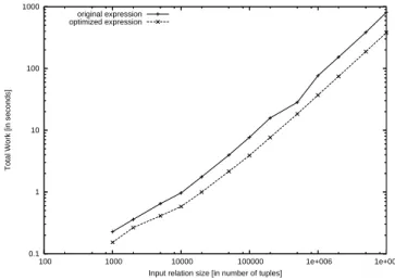
Figure 4: Evolution of total work required for producing the SMALLPAYMENTS relation with an increasing number of tuples.
On all experiments, we test the original expression σpi(µf1,f2,f3,f4(r)) and the
optimized expression µf1,σpi◦f2,f3,f4(r), were predicate pi has some predefined
selectivity and r is an input relation with a predefined size. The results of the experiments performed are presented in graphics using a logarithmic scale on both axis.
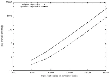
5.2.1 The real-world example
In this experiment, we simulate a real-world scenario that consists of popu-lating the relation SMALLPAYMENTS[ACCTNO, AMOUNT, SEQNO] formed by all pay-ments whose amount is smaller than 50. This relation can be obtained from the relation PAYMENTS presented in Example 1.1. Since, according to Exam-ple 3.1, µacct,amt(LOANS) corresponds to the relation PAYMENTS, the expression
σAMOUNT<50(µacct,amt(LOANS)) denotes the relation SMALLPAYMENTS.
We evaluated the original expression σAMOUNT<50(µacct,amt(LOANS)) and its
equivalent optimized expression µacct,σAMOUNT<50◦amt(LOANS), obtained via Rule 4,
over input relations with sizes varying from 1K to 10M tuples. The results, presented in Figure 4, show a remarkable improvement on total work of the original expression over the optimized expression. On this first experiment, we observed that the optimized expression was evaluated more than 5 times faster than the original expression. The average selectivity of the predicate AMOUNT < 50 was 0.0049, and the observed fanout factor for the amt function
was 101.6. The input relation consisted of a table with one million tuples. 5.2.2 The influence of predicate selectivity
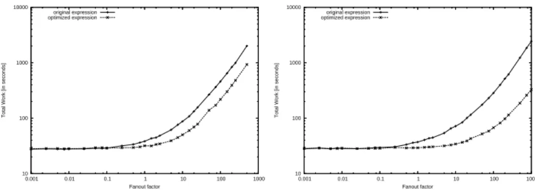
To understand the effect of the predicate selectivity, a set of experiments was carried out using a different pi predicate with selectivity factor ranging from
0.1% to 100%. The tests were executed over an input relation r with 1 million input tuples. Figure 5a shows the evolution of the total work for different selectivities.
10 100 1000 10000
0.1 1 10 100
Total Work [in seconds]
Predicate selectivity factor [in %] original expression optimized expression 10 100 1000 10000 0.1 1 10 100
Total Work [in seconds]
Predicate selectivity factors [in %] original expression
optimized expression
Figure 5: Evolution of total work for the original and optimized expressions with increasing selectivity factors for a mapper with four functions with a fanout factor of 2.0 over input relations with 1M tuples. (a) On the left, the evolution for a single predicate and (b) on the right, the evolution for four predicates.
As expected, the highest gains brought by the optimization were obtained for smaller selectivity factors. More concretely, for a selectivity of 0.1%, the optimized expression was 2.28 times faster than the original. As the selectivity factor decreases, more results are filtered out from function f2 and, therefore,
the cost of computing the Cartesian product involved in the mapper is lower. As the selectivity tends to 100%, the gain drops since the results filtered out from f2 tend to 0%. Nevertheless, there is still, albeit small, a gain dued to
the reduction on the number of predicate evaluations. This gain is small since the cost of a predicate evaluation is, in our experiments, low. If the predicate evaluation is expensive, considerable gains can be achieved even if the predicate selectivity is high.
The modest results for higher predicate selectivities can be combined to produce substancial performance improvements. Consider the case where dif-ferent predicates apply to difdif-ferent mapper functions. The effect of pushing multiple predicates to a mapper function employing Rule 4 is similar to push-ing spush-ingle predicate with a much smaller selectivity. As we have seen above, smaller selectivities impact positively on the achieved optimization. We tested a scenario of pushing multiple predicates to different mapper functions that consisted of pushing a predicate p defined as the conjunct p1∧ p2∧ p3∧ p4.
The original expression used was σp(µf1,f2,f3,f4(r)) and the optimized
expres-sion was µσp1◦f1,σp2◦f2,σp3◦f3,σp4◦f4(r). Figure 5b shows the evolution on total
work when we have four predicates and we vary predicate selectivities. This ex-periment shows that we can obtain good improvements even for relatively high selectivity values. For instance, for a selectivity of 50%, the optimized version is still 45% faster than the original.
5.2.3 The influence of function fanout
To understand the effects of the function fanout on the optimization proposed, we tracked the evolution of total work for the original and optimized expressions when the fanout factor varies. Function f2 was replaced by a function that
guarantees a predefined fanout factor ranging from 0.001 (unusually small) to 200. To isolate the effect of the fanout, the fanout factors of the remaining
10 100 1000 10000
0.001 0.01 0.1 1 10 100 1000
Total Work [in seconds]
Fanout factor original expression optimized expression 10 100 1000 10000 0.001 0.01 0.1 1 10 100 1000
Total Work [in seconds]
Fanout factor original expression
optimized expression
Figure 6: The evolution of total work for the original and optimized expressions with increasing mapper function fanout factors over an input relation with 1M tuples. Predicate selectivity was fixed to 2.5%. (a) On the left, the evolution of total cost; (b) on the right, the evolution of the sum of total cost without materializing the output tuples.
functions were set to 1.0 and the selectivity of the predicate was kept constant at 2.25%. In this case, most of the execution time of the mapper is spent in reading the tuples and executing the mapper functions.
The results, depicted in Figure 6a, show that no visible benefit is intro-duced by the optimization for fanout factors smaller than 0.25. When mapper functions have small fanout factors, fewer tuples are effectively generated and the optimization rule does not have the opportunity to excercise any significant difference.
The performance improvement brought by the optimization increases with the fanout factor. For a fanout factor of 0.25 there is a performance improvement of 8%. This improvement increases to 20% for a fanout factor of 1.0. For a fanout equal to 7.5, the optimized expression is 2.3 times faster than the optimized one and from this point on, the gain increases slightly with the fanout factor. Above this point, the cost of evaluating the predicate, computing the Cartesian product and writing the result are the most important ones in the evaluation of the mapper. The optimized expression only improves the computation of the Cartesian product. For this reason, the gain increases slowly with the fanout. If the cost of writing the result of the mapper in not taken into account, as shown in Figure 6b, the gain improves with the fanout.
5.2.4 The influence of input relation size
We also observed the evolution of the evaluation cost of the original and the optimized expressions when varying the input relation size. We vary the input relation with increasingly greater input sizes ranging from 1K to 1M tuples. Each tuple was guaranteed to have 32 bytes length. In Figure 7, we observe that the influence of the input relation size on total work is linear both for the original and for the optimized expressions and furthermore the gain remains constant.
0.1 1 10 100 1000 100 1000 10000 100000 1e+006 1e+007
Total Work [in seconds]
Input relation size [in number of tuples] original expression
optimized expression
Figure 7: Evolution of total work for the original and optimized expressions when we vary the size of the input relation. The selectivity of the predicate is fixed to 2.5% and the function fanout is set to 2.0.
5.3
Discussion
We have presented three sets of experiments to show the influence of three factors on the improvement brought by the optimization of Rule 4. We have found that predicate selectivities and function fanout factors deeply influence the cost of the mapper evaluation and thus the gain of the optimization. The input table size does not have any influence on the gain achieved by the optimization. Below, we discuss in detail each of these aspects. In the sequel, we also refer other factors that influence the expression evaluation cost.
Both for optimized and for the original (non-optimized) expressions, the cost of the mapper evaluation, either optimized or not is a sum of the cost of reading the input relation, the cost of applying the mapper function to each input tuple, the cost of performing the Cartesian product, and the cost of evaluating, if any, the predicates plus the cost of writing the result.
The cost of reading the input relation, writing the result and evaluating the mapper functions remains equal in both cases. The cost of producing the Cartesian product and evaluating the predicate is lower in the optimized mapper expression. The cost of the Cartesian product is proportional to the cardinalities of the sets of output values produced by the mapper functions. By applying first the predicate and then computing the Cartesian product, we reduce, a priori, the average number of input values fed to the Cartesian product8. At the same
time, we may reduce the number of times the predicate is evaluated. In the non-optimized version, the predicate is evaluated once for each tuple resulting from the Cartesian product. In the optimized version, the predicate is evaluated once for each output value of the mapper function. Therefore, the improvement of the optimized expression is mainly explained because we do not need to build and manage unecessary tuples.
The observations reported in Section 5.2.2 confirm that the application of 8This reduction factor is equal to the selectivity of the predicate.
Rule 4, introduces substantial performance improvements in the presence of predicates with small selectivity. Moreover, although modestly, it is successfull for cases where predicate have relatively high selectivity factors.
The positive effects of increasing the fanout factor together with a low selec-tivity predicate is shown in the experiment described in Section 5.2.3. This is due to the fact that when the fanout is high, the cost of computing the Cartesian product is higher. However, since the predicate selectivity is low, the application of of Rule 4 achieves a high gain, as shown by the experiment.
Input relation size has virtually no influence on the improvement of the optimization. As reported in Section 5.2.4, the total work of both the original and the optimized expressions grows linearly and with the same step. Hence, the improvement is constant on the size of the input relation. Since the I/O time is the same for the non-optimized and for the optimized expressions, we can conclude that computing the Cartesian product of the function outputs, responds linearly9 when the number of input tuples increases.
Other factors that influence the cost of evaluating the expression were con-sidered but not experimented. Namely, the function evaluation cost and the predicate evaluation cost.
Since the proposed optimization does not optimize the function evaluation cost, any increases on the cost of evaluating the mapper functions is added both on the original and on the optimized expressions. A limitation of this optimization lies in the fact that it does not optimize neither the I/O cost nor the cost of applying the mapper functions. If these costs are much higher than the cost of computing the Cartesian product and evaluting the predicate, then the improvements obtained with the optimization are neglectable by comparison with the overall execution time. This was shown in the experiment reported in Figure 6, for a fanout below 1, where the dominant costs are the I/O cost (reading) and the cost of evaluating the mapper functions.
In what concerns the cost of applying the predicate, the gain depends of the fanout of the mapper functions. In the optimized version, we apply the predicate for each ouput value of the mapper function. In the non-optimized version, the predicate is applied for each tuple of the result Cartesian product. The number of tuples produced by the Cartesian product, for each input tuple, is given by multiplying the fanout factors of all mapper functions. In the presence of expensive predicates, for functions with high fanout, high gains can be achieved.
6
Related work
Since Codd’s original paper [10], several extensions to the RA have been pro-posed. There have been two chief motivations for these extensions. First, the type of queries that can be expressed (like aggregates [21] for data consolidation, or controlled recursion for solving problems like the classical bills-of-material [22]) had to be enlarged. Second, new data types (e.g., set-valued attributes [26] or historical, statistical and sensorial data [28]) had to be handled.
Data transformation is an old problem and the idea of using a query language to specify such transformations has been proposed back in the 1970’s with two prototypes, Convert [34] and Express [35], aiming at data conversion.