Master Thesis European Master in Computational Logics

(1)

Universidade Nova de Lisboa Faculdade de Ciências e Tecnologia Departamento de Informática

Master Thesis

European Master in Computational Logics

Multiple sequence alignment

correction using constraints

Luciano M. Guasco

1

EMCL

2

FCT/UNL

3

lucianoguasco@gmail.com

()

Lisboa (2010)

1_{supervised By Dr. Ludwig Krippahl.} 2_{European Master in Computational Logics}

(2)

(3)

Universidade Nova de Lisboa Faculdade de Ciências e Tecnologia Departamento de Informática

Master Thesis

Multiple sequence alignment

correction using constraints

Luciano M. Guasco

4

EMCL

5

FCT/UNL

6

lucianoguasco@gmail.com

₍₎

Orientador: Dr. Ludwig Krippahl

4_{supervised By Dr. Ludwig Krippahl.} 5_{European Master in Computational Logics}

(4)

iv

Trabalho apresentado no âmbito do European Master in Computational Logics, como requisito parcial para obtenção do grau de Mestre em Com-putational Logics.

(5)

(6)

(7)

Acknowledgements

First of all, I would like to thank my supervisor Dr. Ludwig Krippahl for his guidance, advises, continue feedback and enthusiasm to answer my doubts about many topics.

I want to express my thanks to all the CENTRIA people, that accompanied me during my studies in Portugal, specially when we shared many chats at the incredible open houses.

My thanks to the EMCL consortium, for the scholarship I got to complete this stud-ies, money without which it would have been impossible for me to study in Europe.

I would like to give thanks to my family and my friends for their continuous sup-port and the strength transmitted to commit this work.

I also would like to thank my girlfriend. I am really grateful for her continuous moral support and advises.

(8)

(9)

Abstract

One of the most important fields in bioinformatics has been the study of protein se-quence alignments. The study of homologous proteins, related by evolution, shows the conservation of many amino acids because of their functional and structural impor-tance. One particular relationship between the amino acid sites in the same sequence or between different sequences, is protein-coevolution, interest in which has increased as a consequence of mathematical and computational methods used to understand the spatial, functional and evolutionary dependencies between amino acid sites. The prin-ciple of coevolution means that some amino acids are related through evolution be-cause mutations in one site can create evolutionary pressures to select compensatory mutations in other sites that are functionally or structurally related.

With the actual methods to detect coevolution, specifically mutual information tech-niques from the information theory field, we show in this work that much of the in-formation between coevolved sites is lost because of mistakes in the multiple sequence alignment of variable regions. Moreover, we show that using these statistical methods to detect coevolved sites in multiple sequence alignments results in a high rate of false positives.

Due to the amount of errors in the detection of coevolved site from multiple se-quence alignments, we propose in this work a method to improve the detection effi-cacy of coevolved sites and we implement an algorithm to fix such sites correcting the misalignment produced in those specific locations.

(10)

x

based on constraint programming techniques, to avoid the combinatorial complexity when one amino acid can be aligned with many others and to avoid inconsistencies in the alignments.

In this work, we present a framework to impose constraints over the sequences, and we show how it is possible to compute alignments based on different criteria just by setting constraint between the amino acids. This framework can be applied not only for improving the alignment and detection of coevolved regions, but also to any desired constraints that may be used to express functional or structural relations among the amino acids in multiple sequences. We show also that after we fix these misalignments, using constraints based techniques, the correlation between coevolved sites increases and, in general, the new alignment is closer to the correct alignment than the MSA alignment.

Finally, we show possible future research lines with the objective of overcoming some drawbacks detected during this work.

(11)

List of Figures

2.1 Arc consistent graph, but no solution. . . 14

4.1 Visualizer tool, Mutual Information and Alignment . . . 27

4.2 Ratio match, mismatch of coevolved sites in Correct and Clustal align-ment. . . 29

5.1 Variable based representation of sequences . . . 34

5.2 Gap Model: Position Constraint, variables and expressions.. . . 36

5.3 Position Model:Constraints, variables and expressions. . . 39

5.4 A simple alignment and order constraints . . . 40

5.5 The search space is totally expanded for the gaps variables . . . 46

6.1 Sequences and coevolution guessing . . . 55

6.2 Mapping for the sequences in sites I and J . . . 56

6.3 Normalization of the mapping: at left the Map, at right the normalized one . . . 57

6.4 Mistake identification and "canFix" checking . . . 58

6.5 Ratio of detections . . . 63

6.6 Detection using both algorithms for blosum and mapping coevolution. . 65

6.7 Detection using both algorithms for cluster coevolution. . . 66

(14)

(15)

List of Tables

2.1 Two sequences aligned.. . . 4

2.2 Coevolution in pairs of sites: (i,n) and (j,m). . . 8

4.1 Average Pairwise homology score given by Clustal. . . 28

5.1 Conflict if we want to align A’s, and B’s . . . 42

5.2 Gaps Model, set up and execution times. . . 48

5.3 Position Model, set up and execution times. . . 48

6.1 Tests description. Coevolution mutation: blosum, mapping, cluster. . . . 64

6.2 Alignment similarity with correct alignment . . . 67

(16)

(17)

1

Introduction

Many methods have been proposed to understand the evolutionary dynamics of or-ganisms using Multiple Sequence Alignments as the main tool.

Of special interest to this work is the coevolutionary relationships among amino acids in different position of protein sequences, because this relationship shows an evolutionary dependency between these regions.

The importance of correct sequences alignment that include co-evolved sites, stems from the fact that conserved correlation between this sites through evolution from a common ancestor shows a functional or structural relation between them.

During this work we show how the multiple sequence alignment produces mis-takes when aligning the more variable regions where coevolution might have occurred, because alignment algorithm tries to optimize the conservation of sequences, based on static substitution weight matrices, and much of the correlation information is lost after the alignment.

In this work we also show some techniques to discover coevolution, and we pro-pose some improved methods to do so.

(18)

1. INTRODUCTION 1.1. Layout of this work information between coevolving sites.

Constraint programming is a good technique to solve combinatorial problems, since constraint propagation can greatly reduce the search space. In our specific problem, we use constraints to solve many alignment conflicts, pruning the variables’ domains and reducing the search space of allowed alignments. In this work, a framework for han-dling protein sequences and alignment constraints is presented, and it can be used in the future in any problem involving constraints on sequences.

1.1 Layout of this work

In Chapter 2, we give an introduction to the basis and definitions that we use in the next chapters. We explain some problems and previous works on protein sequence alignments, multiple sequence alignment, coevolution, constraint programming, and we also introduce our protein sequences simulator.

In Chapter 3 we present the objectives of this work.

In Chapter 4 we present the mutual information concept, some techniques already explored, and we present our tool for mutual information visualization and some re-sults.

In Chapter 5 we model the sequences in a constraint framework, where we propose some methods for setting constraint and adding dynamic alignment. We also test the methods and show the results.

In Chapter 6 we present a method to disambiguate the uncertainty of which sites are coevolved and we specify a technique for using the method of chapter 5 to fix the alignment. We also test the different algorithms and show the results.

(19)

2

Preliminaries

2.1 Sequence Alignments

A protein sequence is an ordered list of amino acids. The amino acids are biological entities, that we represent as a set of 20 characters. Each amino acid occupies a position, called a site in the sequence. In this work, we focus only on the primary structure level of the proteins, working directly with the amino acids sequences.

Protein and DNA sequencing has become an essential tool in the study of the struc-tures and functions of proteins in any kind of living organisms, to understand cellular processes, and even to study such organisms in many scientific areas such as ecology and species conservation. There are many methods to determine protein sequences, whether from DNA sequencing or working directly with proteins as is the case ofMass spectrometryandEdman degradation.

Once the protein sequences are determined, aSequence Alignmentis a way of com-paring and aligning the sequences according to the amino acids present in the corre-spondent sites, from which some information can be inferred, such as the functional and structural importance of conserved regions and relations between sequences.

(20)

2. PRELIMINARIES 2.2. Algorithms for Sequence Alignment

K L Y E C N E - R S - A

- - - E C N E E R S K A

Table 2.1: Two sequences aligned.

In many representations of alignments, also in table2.1, the sequences are arranged in rows so that the aligned residues, i.e. aligned positions, appear in successive columns. The columns with a total match in the amino acid can correspond to a conserved region in the sequences, information that never changed in the evolution from the common ancestor.

A mismatch in a column can correspond to a mutation, a replacement of one amino acid by other during the evolutionary process through the generations of the species, or it can be a mismatch that can be aligned with the correspondent successive amino acid in the sequences adding a gap.

We can identify the conserved regions as part of the sequences that are perfectly conserved through the linages in the evolution history of the common ancestor. These conserved regions, as proposed in [NH03], suggest that such regions have a structural or functional importance.

The reason whysequence alignmentsare so important in bioinformatics, is due to the identification of sequences similarity that many times is assumed to reflect a degree of evolutionary change from a common ancestor. So, in this case, if we align sequences we can see the differences among them as changes in the evolutionary lineage.

The alignments are important, because they can tell how related two sequences are, and which regions of the sequences they share, generally related to a functional or structural similarity in two sequences. Biologists usually use these alignments to com-pare sequences that have a common ancestor from which they inherit this functionality or structural sections.

Sequence Alignments is a widely used tool in many fields, and many algorithms have been proposed to solve this problem. In this work, we use them to realize some experiments.

2.2 Algorithms for Sequence Alignment

(21)

2. PRELIMINARIES 2.3. Algorithms for Multiple Sequence Alignment same site, or as an indel introduced in some linage, if one of the sequences contains an insertion or a deletion mutation.

In this section we mention the basic algorithms for two sequence alignment and in the next section we analyze what happens when we want to align more than two sequences (Multiple Sequence Alignment).

Finding the alignment between two protein sequences is a complex task that can be tackled with many techniques. These approaches in general in two categories: global alignmentandlocal alignment. Global alignments attempt to align the whole sequences, a form of global optimization that accounts for all regions wether they match or not. Local alignmentsinstead, align those regions which are similar in both sequences and ignore regions that are too divergent.

We mention two approaches based on dynamic programming. One is a global alignment algorithm, Needleman-Wunsch [NW70], and the other a local alignment algorithm, Smith-Waterman [SW81]. We invite the reader to follow the correspondent papers to read more about the algorithms, but in this work it is enough to take into account that these methods are useful when pairwise alignment is needed, in some optimized version of quadratic time.

For both algorithms we need thesubstitution matrixconcept. Asubstitution matrixis a matrix that, for every pair of amino acids, shows a measurement of how probable is that one of the amino acid changes to the other. These matrices are useful when we are aligning, because we should determine if its convenient to proceed over a mismatch with the insertion of a gap or consider it as a point mutation. The substitution matri-ces can be constructed from statistical analysis of many well known sequenmatri-ces where point mutations occur. Actually, many matrices already exist and can be used with this purpose, as it is the case of BLOSUM matrices [HH92]

2.3 Algorithms for Multiple Sequence Alignment

Given three or more protein sequences or DNA sequences, a multiple sequence align-ment algorithm is a method to search the best alignalign-ment of the sequences. It is usually assumed that such sequences share an evolutionary relationship and are descendant of a common ancestor. Also these algorithms can produce a phylogenetic tree with an evolutionary lineage hypothesis.

(22)

2. PRELIMINARIES 2.3. Algorithms for Multiple Sequence Alignment optimal alignment.

There exists a classification of these algorithms according to the way they proceed over the sequences. In the next section we review the most important techniques for multiple protein sequence alignment, pinpointing the advantages and drawbacks of each one.

2.3.1 Dynamic Programming

Dynamic programming technique can be used to produce the globally optimal align-ment. The algorithm receives a set of gap penalties and a substitution matrix assigning scores according to the alignment of each possible pair of amino acids, based on the similarity and the probability of change of them.

For n sequences, the algorithm constructs a n-dimensional matrix, equivalent to the 2-dimensional constructed for 2 sequences as described in previous section. The complexity of the search space increases exponentially when a new sequence is added, as this means a new matrix dimension. The multiple sequence alignment algorithm with dynamic programming technique, tries to minimize the sum of the scores of the matrix giving a way to traverse backward the matrix and determines which sites align with each other, according to the direction of the path, that can fall in a decision of add gap to some of the sequences or leave the partial alignment as it is in that position.

This algorithm has a complexity, governed by the matrix creation step, of O(SN), where S is the length of the sequences andN the number of sequences. As has been shown in [WJ94], the problem of finding optimum global alignment for n sequences using this method, is a NP-complete problem.

2.3.2 Progressive Alignment

(23)

2. PRELIMINARIES 2.3. Algorithms for Multiple Sequence Alignment In the way this method works, the alignment may not be globally optimal because the two most similar sequences are aligned and then this alignment is aligned with the next sequence, and so on. This process is susceptible to propagating the mistakes made in the previous steps to all future alignments with the remaining sequences. This is why in some studies, as [DWFG10], they conclude that the errors in the final result increase for more dissimilar sequences.

One of the most popular MSA application based on the progressive method is Clustal[LBB+07]. Clustal works by calculating all the pairwise distance for the se-quences and constructing the tree from such distances. The pairwise distances can be calculated with a fast and not so precise method, or with one slower but more accurate based on dynamic programming algorithms. With this distance information, the tree is constructed with the cluster algorithms and stored in a dendrogram (a specific guide tree). Then, with the guide tree defining the order, the progressive alignment strategy is applied to obtain the final alignment. The performance of Clustal was determined in [TPP99] and motivate us to test the alignment with the coevolution sequences as we describe in the objectives section.

2.3.3 Iterative Alignment

If we think in the previous method, the progressive one, but now we relax the con-cept that every intermediate alignment is fixed, in the sense that we can adjust it in future alignment steps, we have an iterative method. Mainly we lose efficiency, lack-ing the straightforward steps of the progressive method, but we gain accuracy because a correction procedure is accepted after an intermediate alignment is done.

There are many iterative algorithms, as explained in [Bat05], and they have differ-ent approaches in the way they select the sequence to align and also the correction procedure after the intermediate alignments.

The iterative methods are also heuristic in the search of the best multiple sequence alignment. The idea is that many refinements are done when possible to improve the alignment in each iteration, computing a solution of the problem as a modification of an existing sub-optimal solution, driving to a good but sometimes not optimal solution [Bax05]. Anyway, the final alignments obtained by this methods are robust.

(24)

2. PRELIMINARIES 2.4. Coevolved sites

2.4 Coevolved sites

In a general biological view, coevolution is the change of some state of a biological en-tity triggered or pressured by the change of a related enen-tity. In nature this coevolution appear at many levels, for example in the evolution of two species where a particular change in one of them makes the other evolve and adapt to that change. It is the case of many related species that have coevolved for long time, as hummingbirds and or-nithophilousflowers, orangracoid orchidsandAfrican moths. Although coevolution was also part of Darwin’s work The Origing of the Species [Dar95], where there are many examples of pair of species evolving and adapting in a race against each other, the def-inition of the concept is attributed to Ehrlich and Raven, in a study on butterflies and plants evolution [ER64].

Many techniques have been used to understand the evolutionary dynamics of or-ganisms through the analysis of multiple sequence alignments. Through these studies, the importance of conserved residues and correlated residues started to be a popular topic since the studies focused on protein function and structure.

When performing sequence alignment it is often assumed that a mutation in one site is independent of the remaining sites. In many cases, however, sites are related to others and their evolution is dependent on those. For instance, this can occur when two residues are close in the protein spatial structure and some interaction between them is established. In this case, the evolution of these sites will depend on each other. Thus, a mutation on one of them will create a selection pressure for mutants on the other site, leading to a correlation in their evolution.

In the last few years many studies aimed to uncover coevolutionary relationships in amino acids in protein sequences and how they were arose because of their evo-lutionary importance. For instance, in [FT06] we can see many examples of how the correlations between amino acids are related with the functional role of these residues and why these correlations appear in the evolution of protein sequences.

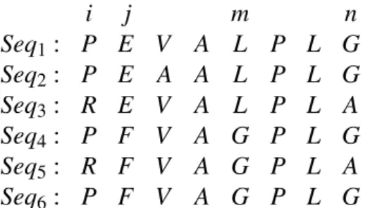
i j m n

Seq1: P E V A L P L G Seq2: P E A A L P L G Seq3: R E V A L P L A Seq4: P F V A G P L G Seq5: R F V A G P L A Seq6: P F V A G P L G

(25)

2. PRELIMINARIES 2.5. Simulated data sets To clarify the concept of coevolution, we can see the table 2.2 that there exist cor-relations between sites i and n, and j and m. We can see how a mutation at site i in Seq3 and seq5 mutate from amino acid Pto R, and force also a mutation in site n for those sequences, mutating from amino acidGtoA. In the sitejthe mutation produces a correlated mutation at sitem, such that every time an amino acid in the sitejmutates, in this case fromEtoF, the correlated sitemmutates fromLtoG.

Coevolution appears when some amino acids are related through evolution because mutations in some sites can cause evolutionary pressures to select compensatory mu-tations in other sites that are functionally or structurally related.

Prediction of coevolution in protein sequences has been studied in many works as [GOP07,WP05,NGR10,FHWE04,FT06]. Some of them work directly on the phyloge-netic analysis, instead of on the alignment itself. Phylogephyloge-netic techniques give an idea about the ancestral relation between the sequences, but this approach of detecting co-evolution based on the phylogenetic trees has the problem of distinguishing between what is properly coevolution and what is just the inheritance of conserved amino acids that differ in different branches of the phylogenetic tree.

Most alignment algorithms use the mutation matrix probabilities and scoring func-tions to align the sites of the sequences. During this work, we examine how coevolu-tion informacoevolu-tion is not taken into account at the moment of the alignment and in many cases losing this information in the final alignment.

In this work we address the calculation of the coevolution using the approach of calculating the mutual information for every pair of sites. We estimate the correlation of sites based on the statistical information in the sequences in a multiple sequences alignment and we consider these sites as the guide sites to detect mistakes in the align-ments.

2.5 Simulated data sets

Since we need protein sequences for which we know the correct alignment and the co-evolved sites to do our experiments with, we developed a protein sequence simulator. Following the previous definition of a protein sequence as an ordered list of amino acids, we constructed an application to generate these sequences and provide an evo-lutionary engine simulator to imitate as best as possible the evolution of sequences in nature.

(26)

2. PRELIMINARIES 2.5. Simulated data sets on the driver, there is a favored state in the driven that will pressure the transformation process.

For the representation of the sequence of amino acids we used the List Prolog con-structor. Each position in the list corresponds to a site, and each element of the list will correspond to a pair (Amino,Pos), where Amino is one of the possible amino acids, and Pos corresponds to an identifier of the site. In the beginning of the simulation, Pos has the value of the position, the site, of the amino acid. But practically this identifier is maintained for future work on the sequences, specifically in the alignment step and while dealing with insertions.

A protein sequence will be a triplet(ID,List,Coevolved), where ID represents the se-quence identifier, List represents the list of pairs (Amino, Pos) in the sequence, and Coevolved correspond to a list of pairs (P1,P2), such that for this given sequence the sites P1, P2 are coevolved. We assume that every site in List that doesn’t belong to any pair in Coevolved, corresponds to an independent site.

The evolution process of the simulator is an iterative transformation of the lists. In the beginning we create one sequence, the root sequence, and then, from this one, we create two offspring through a transformation step. In each step of the iteration, one transformation - as it will be explained later, mutation, insertion or deletion - is applied to each of the two offspring that will replace the parent sequence.

To generate the first sequence, we compute a random assignment of amino acids for each site, following a probability distribution corresponding to the relative frequency of each amino acid, data which is easily available [MB99].

A List of sequences will represent the complete offspring in a certain generation. For each step, to create the next generation, we transform each sequence on the list re-placing it by their two offspring. Each generation containing N sequences will generate in an iteration a population of 2*N sequences.

The insertion in a given position N, corresponds to the insertion of a new amino acid in that place. For this, we shift all the sites, after the N position, to the right on the sequence. We use uniform distribution probability for the selection of the new amino acid to be inserted.

The insertion can cause an incompatibility between the coevolved sites, because now the sequence has a different size and the amino acids were shifted. So, we should normalize the coevolved sites as explained:

• Ff N<=A, for every pair (A,B) in the coevolved list for this sequence add 1 to A and B.

(27)

2. PRELIMINARIES 2.5. Simulated data sets • Do nothing otherwise.

The deletion in a given position N, corresponds to a deletion of the amino acid in the site N, so it is a renaming of the amino acid in such position by a ’-’ character (indel). If the deletion will be done on a coevolved site, it means there exists a pair (A,B) in the coevolved site list of the actual sequence and A=N, or B=N, then the deletion will not have any effect on the sequence.

We simulate the mutation used in the evolution along the offspring with changes in random sites following a BLOSUM62 matrix of transition probabilities [HH92]. BLO-SUM62 transition probabilities is a matrix that contains for row I, column J, the proba-bility of I mutating to J.

We handle the mutation of a coevolved site for a given sequence like other re-searchers do in [GOP07]. As we know, the coevolved sites are pairs (A,B) such that A is the driver, B is the driven. This means that the driver site will press on the mutation of the dependent site, and this pressure will correspond to a selection of favored state in the driven given the state of the driver, with a certain level of pressure corresponding to a coevolution factor.

We implemented the coevolution method in three different ways. In the Most Prob-able Cluster method, as specified in the work [GOP07], the amino acids were grouped into 7 different clusters, corresponding to the evolutionarily most meaningful division of them. Each site will evolve according to BLOSUM62 matrix index with the actual amino in the site to mutate (the first element in the pairs of blosum buckets), but the choice won’t be done over all the possible mutations for this amino acid, but only for those which are in the same cluster as the driver amino acid. The clusters were obtained using a non-hierarchical clustering method, k-means, on the matrix BLO-SUM62 and yielding the evolutionary most meaningful division of amino acids. The next method, Blosum Coevolution, will be a mutation guided by the Blosum matrix. The idea, is to get from the Blosum distributions the mutation correspondent to the driver and also the new amino acid distribution that will pressure on the correspon-dent coevolved site mutation. The third one is just a strict mapping, from the most probable evolution of one amino acid to other one, purely experimental for our future work but that we construct from the probabilistic mutation matrix adding biological meaning.

(28)

2. PRELIMINARIES 2.6. Constraint Programming

2.6 Constraint Programming

Aconstraintcan be seen as a logical relation among many entities, each of them taking some values from their specific domain. The constraints are responsible for restricting the values the entities can take. One of the flexibilities of the constraints is their hetero-geneous application to different domains for different type of entities, restricting and relating many domains of a problem.

In the last years, Constraint Programming has been a really focused research area in Computer Science and other fields, because it works in a declarative way, providing tools for specifying the relationship that should be maintained in the system, through relation over the variables that take values from their domain, without specifying the computational process through which the relations are assured.

In the same way as we use constraints daily, for instance when we are reasoning or planning: "I will take the metro. In Cais do Sodre station I have to leave before 1pm, and then I have to take the boat before 1.30pm", Constraint Programming is a tool for integrate constraint relating objects in computational systems, assign values to these objects according to the rules that the constraints define and a search for a respective solution.

2.6.1 Constraint Satisfaction

A constraint satisfaction problem (CSP) can be defined as:

• a set of variablesX ={x1,x2, ...,xn},

• each variable is associated with a domain, so for eachxi,Di is a finite set of pos-sible valuesxican take. Depending the framework, the domain of each variable can be of one of many types asinteger,boolean,range,etc., and

• a set of constraints, C, logical relations, that restrict the values the variables can simultaneously take.

In this definition a constraint can be defined as a subset of the cartesian product of the domain of the variables that are involved in that constraint.

(29)

2. PRELIMINARIES 2.6. Constraint Programming The solution can be found by searching systematically, traversing all the possible assignments of values in the domain to the correspondent variable. Since this is not the most efficient way of obtaining a solution, many techniques were proposed during the last years, as many variants of backtracking, consistency techniques, constraint propagation and optimizations among others.

The classic CSP as described above, defines the satisfaction of each constraint as a necessary condition to the solution of the CSP. This restriction means that each con-straint is imperative, each solution satisfies them, and in a total assignment for all the variables, they must be completely satisfied. But these strict assumptions can be re-laxed, as in Flexible CSPs, allowing solutions that do not satisfy all the constraints but only a subset of all constraints.

In this work we work with Max-CSP, where some constraints are allowed to be violated, and the solution is searched through a qualification over the amount of con-straints satisfied. AlsoWeigthed-CSPis considered in this work, aMax-CSPwhere the violations of the constraints are weighted according to some criteria and those with more weight are the ones preferred to satisfy.

2.6.1.1 Consistency techniques

Consistency techniques are approaches to speed up the solution of a CSP, based on the principle of removing inconsistent values from the variables’ domains, reducing the search for consistent labellings. The inconsistencies can appear in the labelling of a variable because the value assigned is inconsistent with such variable, or with the logical relation over the variables, or with some more complex connection.

This techniques are deterministically computations through which values are re-moved from the domain of the variables, and any non-deterministic computation is done once there is no more propagation to do with the consistency techniques.

We will define the different techniques based on unary and binary constraints, due to the fact that n-ary constraints can be transformed to equivalent binary CSP [BvB98]. So, given the CSP we can define:

• Node-Consistency: It removes values from the variables’ domain that are incon-sistent with unary constraints defined over such variables. So, for every value d ∈Di, such that Xi taking the valued make unsatisfiable an unary constraint U, Di =Di− {d}. For instance a constraint positive(X) that states that values in the domain that are below 0 are removed.

(30)

2. PRELIMINARIES 2.6. Constraint Programming

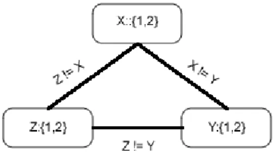
onXi, there is some value, called a support for vi, in the domain ofXj, such that Xi=viandXj=vjis not unsatisfying the constraintarc. The idea of this technique is that if arc-consistency is entailed by the binary constraint, then the values of all variables’ domains that have not support on other variables related by the constraint can be removed from their respective domain. As an example, we can see figure2.1where the nodes represent the variables, labeled with the domains, and the edges are the constraints and we can see the steps for enforce the arc-consistency.

Several arc-consistency algorithms were proposed as in [BR97], from 1 to AC-7. They are all based on the same principle, repeated revisions of the arcs, until a fixed point is reached with a consistent state, or some domain become empty making the constraint unsatisfiable.

Arc-consistency removes many inconsistencies from the constraint graph, but it doesn’t mean that if all the constraint in the CSP are arc-consistent, there exist a solution for such CSP. The idea behind arc-consistency is the reduction of the domains on those values that will never be part of a solution. This can be seen in the example of the figure2.1, where arc-consistency is achieved but there is no solution for this CSP.

• Path-consistency: Beyond the values removed by node-consistency and arc-consistency, more values can be remove from the variables’ domain with path-consistency. It requires for every pair of values, of two variablesXi,Xj, satisfying the respective binary constraint, that should exist some value for each variable along a path fromXitoXj, such that all binary constraint in the path are satisfied.

There are many algorithms proposed to enforce path-consistency, like revisited in [Sin95], but in many situations dependent of the problem, the computational cost to enforce this consistency is not justified against the gain in the speed of the search for a solution.

(31)

2. PRELIMINARIES 2.6. Constraint Programming Most consistency techniques are not complete, so there is no completeness bound-aries to increase the efficiency of the algorithms losing some power in the value re-moval. Some cases of directional arc-consistency, for instance, require that the variables be ordered for working with efficiency and efficacy for constraints that previously en-forced this criteria.

2.6.1.2 Constraint Propagation

The consistency techniques explained before, are not always sufficient for finding a solution or proving any CSP unsatisfiable. Instead these are methods that use each constraint or set of constraints to satisfy a local consistency between the variables they are associated with. Instead of using isolated techniques, a combination of local con-sistency and systematic search is in general used to search for the solution.

There exist many variations of the backtracking algorithms, asbackmarking[Pro95] that reduce the number of redundant checks by remembering previous incompatible labellings.

Also there are many variations of look ahead approaches, methods that prevent future conflicts analyzing the actual status and checking possible new states. As ex-plained in [RBW+]Forward Checking, andPartial Look Aheadare the most common look ahead techniques and they combine arc-consistency, or directed arc-consistency, dur-ing the search enforcdur-ing that there exist possible values for future variables to be ex-plored.

Many techniques for increasing the efficiency of constraint propagation are based on the search strategy, in which the order in which the variables are labeled is defined, i.e. a deterministic way is imposed. Also, the domain of the variables can be explored by the labeler in different ways, according to the problem, and extracting the values to assign with a specific criteria, as the maximum value, minimal value, etc. These techniques are really dependent on the problem, and how its modeled with constraints, but they add some efficiency when the solver is searching for a solution.

2.6.2 Constraint Optimization

The goal behind constraint optimization, is not just to find a solution but to find a good solution, measuring its quality by an application dependent function calledobjective function. The solution is searched satisfying the constraints, and also minimizing or maximizing the objective function.

(32)

2. PRELIMINARIES 2.6. Constraint Programming value. It is an under estimation (in case of minimization) of the objective function for the best solution (complete labelling) that can be obtained from the actual partial la-belling. The algorithm proceeds reducing the space of possible solutions, and proceed in a deep search on them. As soon as a value is assigned to a variable, the value of the objective function is calculated for the new labelling, and if its value exceeds the bound, then this subtree is pruned immediately. The bound is started as a big number (in case of minimization), and stores the objective function value for the best solution found so far. So the main idea is to discard all branches that, from the partial state, we know will not generate a solution better than one obtained before.

The efficiency of branch and bound is based on the quality of the objective function, and also on whether a good bound is found early in the search process.

2.6.3 Constraints

There are many type of constraints, and in general, they are classified by the variables they relate. As explained in the node-consistency, the unary constraint relate one vari-able. Binary constraints relate pairs of variables. Many binary constraint are already define with their respective consistency and propagation techniques and in this work mainly we use:

• eq:x=y. Equality constraint, that forces the two variables to take the same value. Enforce Arc-Consistency.

• lt:x<y. Strictly less than, forcing variable x to take a value that is strictly smaller than y. Enforce Arc-Consistency.

.

Global constraints is the class of constraints that relate more than two variables. In general these constraints enforce arc-consistency, and path-consistency could be en-forced losing some efficiency. In this work we make reference to three arc-consistent global constraints:

• allDi f f erent(X1, ...,Xn): states that the arguments have pairwise distinct values: X1 6=Xj; ∀i6= j, This version of the global constraint, is equivalent to pairwise comparison but considering all variables at same time, giving rise to better prop-agation, with specific efficient algorithms. Further in this work we analyze this constraint for future research in Chapter 7.

(33)

2. PRELIMINARIES 2.6. Constraint Programming all variables in x) : low[v−min]≤ |{i|Xi=v}| ≤up[v−min], ∀value v. low and up are the lower and upper occurrence value arrays for each possible value of the variables in the vector X.

• increasingNValue(X1, ...,Xn,N): states that the variablesX1, ..Xntake increasing val-ues, and moreover it forces N to be the number of different values taken by the variables. So, if we impose N equal to n, then X1<X2, .., <X3<Xn. Otherwise, some consecutive variables can take the same values.

(34)

(35)

3

Objectives

Our objective is to conceive and implement techniques, integrated as a single tool, to help in the identification of coevolved sites in Multiple Sequence Alignments (MSA), improving the detection of these sites and the correction of errors in the MSA, in those sites that lost the coevolution correlation.

We start by showing that the alignment algorithm produces mistakes on the coe-volved sites. To do so we need a framework for measuring the information of sites that a priori we know have coevolved in multiple sequences to which we apply a standar MSA tool(Clustal). Due to the size and number of sequences and the lack of a tool to visualize correlation values calculated from the alignment, we need to develop a framework to systematically analyze where and how the mistakes occur to proceed to achieve our goals.

We want to detect this lost coevolution information as consequence of the alignment process. To do this, a protein sequence simulator was developed, which can create a data set with different types of mutations and coevolution schemes, based on the ideas proposed in [GOP07], and it can also indicate the correct alignment for the sequences generated.

(36)

3. OBJECTIVES

that contain coevolution information, since conserved regions cannot show evidence of coevolution.

Based on our tool for detection of possible coevolved sites using a statistical method, we want a better approach to distinguish those sites that have really coevolved from those that have not but are detected as possible candidates due to correlation that arose by chance or by misalignment produced by the MSA algorithm during the alignment. Then, we need a constraint framework that give us the flexibility to set some relations among the amino acids in the sequences, adding a dynamic method to define our cri-teria of alignment. This framework can be our tool to test techniques for the correction of misalignments in variable regions that have coevolved.

(37)

4

Mutual Information in Sequence

Alignments

In this chapter we cover the concept of Mutual Information. We use it specifically to detect apparently coevolved sites, due to the property that indicates coevolution: correlation. Since we are searching for coevolved sites in multiple sequence alignment, mutual information is a good measure to realize this task.

During this chapter, we will explain how this measure closely relates the informa-tion in each site to the coevoluinforma-tion with other sites. Given the difficulties raised bythe errors in the alignment of variable regions, we introduce in this chapter also some techniques to overcome these drawbacks and we show their benefits.

(38)

4. MUTUALINFORMATION INSEQUENCEALIGNMENTS 4.1. Mutual Information Definition

4.1 Mutual Information Definition

Mutual Information measures the amount of information related between one random variable to another one. It appeared first as part of Shannon’s work [Sha01] and has become an important tool inside the Information Theory field.

Mutual Information, over two random variablesI,J,MI(I;J), measures in some way the information that the two variables share. It is an uncertainty measure between what we know about one variable and the information that is in the other.

If I and J are two independent random variables then our measure of mutual infor-mation is zero, because even if we know one of them, we do not have any inforinfor-mation about the other. If both variables are identical, and so always take the same values, our mutual information measure is the uncertainty of one of them, because knowing I we know J and vice-versa. This, knowing one will give us the information about the other that is necessary to reduce the uncertainty to zero. As we will see below, the uncertainty of each random variable is measured by the entropy, so in this case the mu-tual information between Xand Y will be determined by the entropy of any of these variables.

MI(I,J) =

_∑

a∈I

∑

b∈J

PIJ(a,b).log(

PIJ(a,b) PI(a)PJ(b)

) (4.1)

This equation is equivalent to one based on Shannon Entropy concept, and is part of the work in [Sha01]

MI(I,J) =E(I) +E(J)−E(I,J) (4.2)

Where E(I),E(J)refers to the entropy of site I and J respectively, andE(I,J) the join en-tropy ofIandJ, and what formulated in terms of entropy is,

MI(I,J) =−

_∑

a∈I

pI(a)log(pI(a))−

∑

b∈J

pJ(b)log(pJ(b)) +

∑

a,b∈I,J

pI,J(a,b)log(pI,J(a,b)) (4.3)

(39)

4. MUTUALINFORMATION INSEQUENCEALIGNMENTS 4.2. MI Calculation

4.2 MI Calculation

In our work, mutual information is used to compare two sites in the multiple sequence alignments, and measure the related information between these sites. It means that two sites are correlated with a high mutual information value, if the existence of one specific amino acid in a site determines the existence of another specific amino acid in the other site, which suggests a functional or structural relation between the sites.

This measure of MI can give us a clue about which sites coevolved in a set of se-quences that are evolutionary related. One mutation in one site will select for a com-pensatory mutation in other site and this correlation will be kept in the lineage of the sequences.

Intuitively we can calculate the probability of each amino acid occurring in a site I, as the frequency of such amino acid in I over the total amount of amino acids in I (equivalent to the total amount of sequences).

What we are trying to do in this work, is to detect those sites in the multiple se-quence alignment that indicate a possible coevolution, and for this we do the N(N−1₂ ) calculations of mutual information between the sites I,J.

Algorithm 1MI Calculation

1: Freq←empty

2: Freqi j ←empty ⊲Initialization of the HashMap to count amino acid and pairs

3: forsitei=0..LongSequencedo

4: for j=0..NumberSequencesdo

5: Freq(i)←Amino[i][j] ⊲Freq count the aminos in sites i. Amino[i][j] is the amino of the sequence i, in position j.

6: end for 7: end for

8: forsitei=0..LongSequencedo 9: for j=i+1..LongSequencesdo

10: fork=0..NumberSequencesdo

11: Freq(i,j)←(Amino[i][k],Amino[j][k])⊲Freq(i,j) count the pair of aminos in sites i,j

12: end for

13: end for 14: end for

15: forsitei=0..Longsequencedo

16: forsite j=i+1...LongSequencedo 17: MI[i][j]←MI(i,j)

18: end for 19: end for

(40)

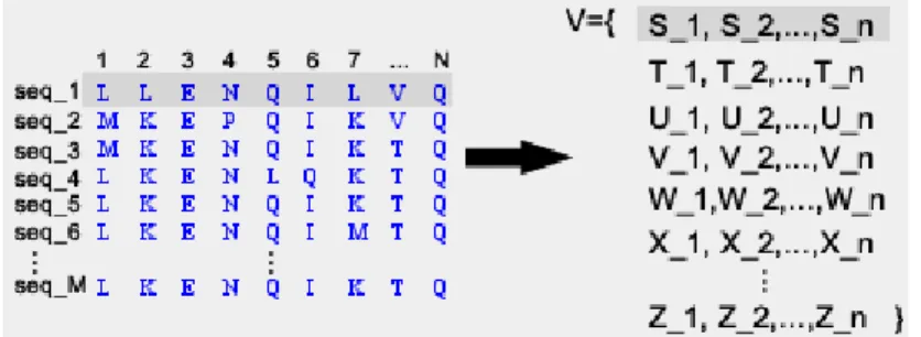
4. MUTUALINFORMATION INSEQUENCEALIGNMENTS 4.3. Normalization of the MI each site, and other one to keep the amount of amino acids pairs in each pair of sites. First, we traverse all the sites and for each sequence we extract the amino acid on such position, adding it to the structure. We do the same for all the pairs i,j of the n(n−1₂ ) combinations of different pairs of sites.

With this mutual information matrix, we can guess the coevolved sites over the evolutionary lineage just by taking the values that are over a threshold T. To use of this information in the analysis of mutual sequence alignments we also developed a visualization tool that allows the matrix representation to be displayed on the screen with a scale of colors representing the amount of MI between each pair of sites and also a correspondence between each cell in the matrix and the sequence alignment result.

As we show in the section 4.5, the threshold T can be estimated after some ex-periments with simulated coevolved sites and analyzing the results of the algorithms. Moreover, we use several normalizations from [GOP07, NGR10] to tune the mutual information equation4.1and get better results in guessing coevolved pairs.

4.3 Normalization of the MI

To detect correlation on sites using the mutual information calculation we have to use some techniques to normalize equation 4.1. For instance, the wide range of possible value for the number of different aminoacids in a site, the logarithmic base we use in the formula, or the calculation of correlation for totally conserved sites, can produce mistakes of good possible candidates of coevolved sites when they are not.

Some solutions to the normalization problem has been proposed in [GOP07]. In the next sections we will explain some models to normalize the values, and we will conduct an analysis of which of the models better solves our problem, showing results that justify our choice according to our calculations.

4.3.1 Adaptable logarithmic base

In the equation4.1 we can postulate that the MI value will fall in the range from zero to one, if we can guarantee three conditions each time we calculate MI between two sites. First, that there is perfect co-variation in each site, i.e. that every amino in one site is co-related with other amino in the other site, and there never exists a pair that does not follow this correlation. Second, the 20 amino acids are present in both sites, condition needed because of the base used in the logarithm of the formula4.3. Third, the 20 different amino acids are present in equal frequencies in both sites.

(41)

4. MUTUALINFORMATION INSEQUENCEALIGNMENTS 4.3. Normalization of the MI important for the coevolution detection is the first one, and the other two, even though when present in the formula the detection of coevolution is still working, they also decrease the quality of the detection of the coevolution if it is not normalized.

One solution to counter the second condition, is known as Mutual Information of Adaptable Logarithmic Base (MI Adp):

MI(I,J) =∑a∈I∑b∈JPIJ(a,b).log(

PIJ(a,b)

PI(a)PJ(b))

log(sqrt#i.#j) (4.4)

where#irepresents the number of different amino acids occurring in siteAand#j in siteB.

With this formula, we can calculate the MI of two sites obtaining results ranging from zero to one, but independent on the number of different amino acids in each site.

4.3.2 Simple Correlation

With the previous method we can calculate the MI independently of the number of different amino acid in each site. Now, to add independence of the third condition, in order to calculate Mutual Information without influence of the amino acid distribution in the correspondent sites, we apply the following approach.

The influence of the amino acid distribution is due to the entropy calculation, using the logarithm. As explained in [GOP07], the logarithm equation:

− n

∑

i

(xlog(x)) (4.5)

has its maximum atx=1/nwith0<x<1. In terms of amino acids and probabilities it has its maximum when they follow a uniform distribution on the site.

We can use a logarithm independent formula:

MI(I,J) =

_∑

a∈Ib∈J

∑

PIJ(a,b)2 PI(a)PJ(b)

(4.6)

(42)

4. MUTUALINFORMATION INSEQUENCEALIGNMENTS 4.3. Normalization of the MI definition, conserved sites provide no evidence that mutations at one site selected for particular mutations at the other.

The solution proposed in [GOP07] is just to do the whole calculation of MI for every pair of sites, and after that check the existence of conserved sites to which the MI value is modified to zero.

4.3.3 Entropy division

We seek to remove the noise from the first formula4.1, keeping the scores of coevolu-tion deteccoevolu-tion as high as possible and expanding the model to remove the false posi-tives. In some of the methods stated before we have to increase computation time to remove false positives and get a better accuracy.

We can still have a better coevolution accuracy without increasing computation time. We can observe on equation 4.2, that coevolved sites will have similar entropy individually and also similar to the joint entropy. So, one solution is to normalize the formula, dividing the equation 4.1 by the maximum entropy in one of the two sites, obtaining:

MI(I,J) =E(I) +E(J)−E(I,J)

max(E(I),E(J)) (4.7)

This normalization works well when we know that the number of different amino acids in the sites is not large. Evolutionarily, it means that the amino acids in such sites did not mutate many times to different amino acids, but instead they kept within a small group of amino acids. As proposed in the literature [GOP07, FHWE04, FT06], if we are doing a multiple sequence alignment with evolved sequences, this is the behavior we expect to find for coevolved sites.

When one site mutates at a higher rate than the other and changes to different amino acids, it has a higher entropy. Thus, the division by the maximum entropy of the two correspondent sites will maximize the MI when the sites have similar entropy and are correlated, and will decrease the MI when they have different entropy values. This method adds some noise when the entropies differ in an almost related coevolved site. We show in section4.5how this measure is used to classify pair of sites as possibly coevolved ones through a highest scores selection.

(43)

4. MUTUALINFORMATION INSEQUENCEALIGNMENTS 4.4. Visualization tool

4.4 Visualization tool

Once we apply the Clustal alignment and we calculate the MI for all the sites in the MSA, we need a tool to visualize the MI score and the sequences alignment.

This motivated us to develop a visualizer during this work, to pinpoint character-istics in the misalignments over which we drive our work in next chapters.

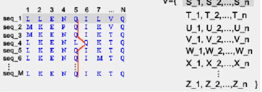
As we show in figure 4.1, the tool shows the pair of sites in a symmetric matrix representation, where each(i,j)cell correspond to the MI value for the sitesiandj. We calculate for any MSA, the n∗(n−1₂ ) different combination of sites(i,j)and we store in the matrix the MI(i,j) with any of the methods presented above. In the visualization we can see a value scale, from 0 to the maximum value the MI can take (according to the method). Also the tool provides a direct visualization of the sequences, and if one pair (i,j)is selected in the MI matrix, then in the sequences visualization these sites are also highlighted for fast identification.

Figure 4.1: Visualizer tool, Mutual Information and Alignment

4.5 Results

(44)

4. MUTUALINFORMATION INSEQUENCEALIGNMENTS 4.5. Results

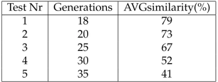
same conditions.) Generations indicate number of iterations for the simulation, and AVGsimilaritythe average similarity score correspondent to the Clustal pairwise score average, which represent the average sequences homology for each test. The genera-tion was done with the coevolugenera-tion method mapping, as described in Secgenera-tion2.5. In each sequence we have 20 pairs of coevolved sites, each sequence is 100 amino acids long and we keep 70 sequences, randomly selected from the last generation of the sim-ulation.

Test Nr Generations AVGsimilarity(%)

1 18 79

2 20 73

3 25 67

4 30 52

5 35 41

Table 4.1: Average Pairwise homology score given by Clustal.

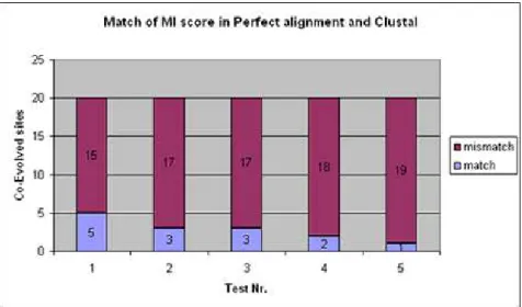
We proceed by calculating the Mutual Information for all the pair of sites, in the correct alignment and in the Clustal alignment. Then for each pair of coevolved site in the test, we compare the MI score marking a match if in both alignments the score is the same and as a mismatch otherwise. Of course, in the correct alignment we get the original information, so if the sites are coevolved and this is reflected in the mutations, the site has a large MI score. If the sites are never mutated, and just conserved, the MI score is really low event if they were marked as coevolving sites in the simulation. But in this experiment we do not pay attention to the MI score itself but only on the differences between correct alignment and the Clustal alignment for the coevolved sites.

(45)

4. MUTUALINFORMATION INSEQUENCEALIGNMENTS 4.5. Results

Figure 4.2: Ratio match, mismatch of coevolved sites in Correct and Clustal alignment.

and False Negatives for sites detected as coevolved sites, showing also that many mis-takes are done over the alignment in such sites, and that the statistical method for co-evolution detection are too sensitive to such noise to be used for detecting coco-evolution without further corrections.

(46)

(47)

5

Alignment using Constraints

In this chapter, we propose two models that can be used to align sequences with im-posed constraints. These alignments are based on desired criteria, for instance, for ev-ery sequence each amino acid in a site should match, if possible, the same amino acid in the next sequence at the same site. Moreover, we establish an alignment framework to work with on the next chapter.

We explore the use of constraints to define possible situations on the alignment and discard unsatisfied states in the search for a solution. We also identify the problems each model has in the alignment process, extending some features to avoid these ob-stacles. Since many constraints can be unsatisfied due to conflict with other constraints, we adapt the models as MaxCSP problems obtaining a system that can handle viola-tions on the constraints, i.e. in the alignment specificaviola-tions, getting the best possible alignment corresponding to the maximum amount of satisfied constraints.

We also present some experiments with multiple sequences and we evaluate the models introduced in this chapter with the goal of detecting the drawbacks and ad-vantages of each of them leading to our selection of a framework.

5.1 Motivation

(48)

5. ALIGNMENT USINGCONSTRAINTS 5.2. Preliminary definitions framework where we can align the sequences using constraints because with the ex-istent algorithms for sequences alignment, we do not have the flexibility to relate the positions where coevolution occurs and force those positions to align not following the typical score matrix but a particular correlation instead. For instance, in Dynamic Programming MSA, the search for the best solution is done expanding the values in the table in an incremental manner, but if we find a state that conditions the change of some state previously calculated, we can not go back and then go forward again as often neded without paying a computational cost and without changing the algorithm to handle any specific optimization alignment.

Having a framework to set constraints in the alignment provides a flexible tool to experiment with the sequences adding dynamical properties that they have to main-tain according to our desire. We need to add this flexibility because we want to deal with the correlations present in the coevolved sites.

5.2 Preliminary definitions

As we want to formalize the models and compare them, we need to establish a com-mon language to talk about the amino acids, sequences, alignments, mismatches, and so forth. We discussed about many of these concepts in the chapter2, but we need to organize them with more formal specific definitions.

Definition 1. We callΣto the alphabet, a finite set of characters. We can define also ΣG, an extension such thatΣ_G=Σ∪ {−}, where−represents a gap in the alignment.

In this work, and from now on, the alphabet corresponds to the set of amino acids because we work over protein sequences, but it can correspond, for instance, to the nucleotides in DNA sequencing.

Definition 2. We define asprotein sequence s, during this work also called justsequence, to a finitestringor finite ordered list of elements over an alphabetΣ. More formally,s= (Σ)∗.

Definition 3. We define asalignment sequencesA, to a finitestringor finite ordered list of elements over an alphabetΣ_{G. More formally,}sA= (ΣG)∗. We define this as an extension of the protein sequences where gaps are added in order to align with other sequences.

Definition 4. Letsbe a protein sequence,s=a1,a2, ...,anwhere∀0<i<n, ai∈Σ. LetsAbe an alignment sequence,sA=b1,b2, ...,bnwhere0<i<n, ai∈ΣGWe can define the following operations over s, and oversA:

(49)

5. ALIGNMENT USINGCONSTRAINTS 5.2. Preliminary definitions • sA(i) =bi. Thei-thelement for an alignment sequence, that belongs toΣG.

• lg:(Σ)∗→N_{. Given the protein sequence}_s,_lg(s)_{calculate its length.}

• lg:(Σ_G)∗→N. Given the alignment sequencesA,lg(sA)calculate its length.

Definition 5. Given an alignment sequencesA,sA∈Σ∗G, the projection ofsA w.r.tΣ, noted as sA|Σ, is defined assAwith the deletion of all the occurrences of ’-’.

Definition 6. Given two or more protein protein sequences,s1,...,sn, we can define a multiple sequence alignment as an-tuple(s1A,...,snA), such that:

• s1A, ..., snA ∈(ΣG)∗.i.e., they are n-alignment sequences.

• s1A|Σ=s1,...,snA|Σ=sn

• lg(s1A) =...=lg(snA)

• ∄i 0<i<lg(s1A) =...=lg(snA) s.t. s1A(i) =...=snA(i) =′−′.

Definition 7. From now on, when we talk about multiple sequences (multiple sequence align-ment), MS (MSA) of size m, we are making reference to a collection of m protein sequences (alignment sequences).MS=s1,s2,s3, ...,sm

We have a formalization of the the multiple sequence alignment, that helps guide our description of the methods for alignments using constraints. Moreover, we need to formalize some concepts in each respective model that we present in this chapter, with a specific semantic.

Definition 8. We can define a set of variables,V, whose elements are variables in the domain [0..N]. When we work on particular domain we specify the meaning of the value N.

Definition 9. A sequence of variables, or Variables, is defined as a succession of different variables of V. Formally:Variables=X1,X2, ...,Xnsuch that,Xi∈V.

Then, we need to map the multiple sequences onto a set of variables. We can do it in the following way:

Definition 10. A mapping, Vars, from a protein sequence to a collection of variables, is defined asVars:Sequence→Variablessuch that∀i ,0<i<n, ifai∈Sequence,then∃Xi∈Variables. The idea is that for different sequences, we will have different set of variables, such thatV =

S

(50)

5. ALIGNMENT USINGCONSTRAINTS 5.3. Gaps Model

In other words, if we have a multiple sequence MS, we have as many sets of vari-ables as sequences in the MS, and all the varivari-ables in all the sets are different. So, every variable represents univocally one amino acid in one sequence.

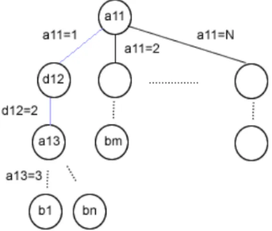
Actually what we define is a way of representing the elements of the sequences as variables over which we work in the next sections. In other words, we can have a mapping from the sequences to sequences of variables, as shown in the figure5.1. This representation is useful for the next section where we give the correspondent semantic for such variables.

Figure 5.1: Variable based representation of sequences

5.3 Gaps Model

5.3.1 Semantic

The goal of this model is to assign the correspondent semantic to some elements de-fined above, with the objective of represent gaps between the amino acid of an align-ment sequence and do an alignalign-ment based on constraint over such gaps.

First we need to add the semantic to the set of variables V. In this model we use the variables to represent the amount of gaps in a certain position. Given the set of variables, from now on, gap variables V with their respective domain [0...N], we can represent gaps between any pair of amino acids ai−1 and ai with the correspondent variableXi, assigning values from the domain to this variable.Nis a constant defining the maximum-length of gaps between consecutive amino acids. For the first element of the sequence,a1, the meaning of the value ofX1is the gap length in the beginning of the sequence, i.e. before the first amino acid.

(51)

5. ALIGNMENT USINGCONSTRAINTS 5.3. Gaps Model Before we proceed with the definition of the constraints for the position of the ele-ments in the sequence, we need to define the concept of position.

Definition 11. We can define a position offset of an amino acid with respect to the beginning of a sequence s, as a function Poss :ΣG−>Expression, i.e. a function with domain in all the possible amino acids and image in Expression, that corresponds to a constraint Expression, defined recursively as:

• Poss(a1) =X1, X1 ∈Vars(s), i.e. ai is the first amino acid in the sequences s and the equivalent expression is the first variable in Vars.

• Poss(aj) =Poss(ai) +Xj+1iff s(j) =aj, s(i) =ai, i< j. i.e., for any amino acid that is not the first one, we calculate the expression as the position of the previous amino acid plus the variable corresponding to this amino acid plus 1.

Note that this function is defined only for the elements of the sequence s. The idea of this function is that, given an amino acid in a sequence, we can get an arithmetic expression that is based on some gaps variables and that locates an amino acids in a se-quence, when the gaps variables take values. Any amino acid position in the sequence is in function of the gaps variables that identify such amino acid and the amount of previous variables and amino acids.

What motivates us to define this position function is the necessity to formalize the concept of the expressions, because this is what we want to constraint when we search for an alignment. When we want to align an amino acid with another located in other sequence, we can force their position expressions to be equal. As we explain later, we write all the alignment desires as a set of constraints.

Definition 12. We define a Position Constraint, PC, over two amino acids at position iandj in two sequences respectivelys1ands2as a constraint on the position of the amino acids. This Position Constraint relates with an operator the position of the two amino acids.

PC(s1(i),s2(j)):Poss₁(i) = Poss₂(j),

(52)

5. ALIGNMENT USINGCONSTRAINTS 5.3. Gaps Model

Once we have defined all the constraints on the position variables corresponding to the desired alignment, we can solve the constraints over the variables’ domains and get a solution for that alignment.

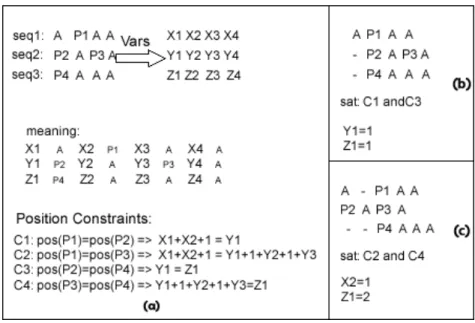
We can see graphically in Figure5.2(a) some position constraints that we can require for an alignment. In this case we want to align the amino acid P1with P2orP3, and P4withP2orP3. We also show some possible alignments, in5.2(b)(c), that satisfy our intended alignment defined by constraints. We can see the expressions obtained when applying pos(Pi). In this figure we do not show how we solve the constraints nor the labelling process because these topics are explained further on.

Figure 5.2: Gap Model: Position Constraint, variables and expressions.

To transform back the values of the variables into a multiple sequence alignment, we have to add the corresponding value for each variable to the position they repre-sent. The main idea is that from protein sequences we create alignment sequences, i.e. the same protein sequences plus the gaps in the corresponding positions according to the value of the variables. To do so, we can define the following function:

Definition 13. We define a functionTrans f orm:Sequence x V→Alignment Sequence, such that:

• Trans f orm(s,V) =sA s.t s′=val(V1)a1...val(Vn)an ∀ai∈s, whereViis the variable associated with the amino acidai, andval(Vi)is k times ’-’, if k is the value that the solver gives to this variable.

Master Thesis European Master in Computational Logics

Master Thesis

European Master in Computational Logics

Multiple sequence alignment

correction using constraints

Luciano M. Guasco

EMCL

FCT/UNL

lucianoguasco@gmail.com

()

Master Thesis

Multiple sequence alignment

correction using constraints

Luciano M. Guasco

EMCL

FCT/UNL

lucianoguasco@gmail.com

()

Acknowledgements

Abstract

Contents

List of Figures

List of Tables

1

Introduction

1.1

Layout of this work

2

Preliminaries

2.1

Sequence Alignments

2.2

Algorithms for Sequence Alignment

2.3

Algorithms for Multiple Sequence Alignment

2.3.1

Dynamic Programming

2.3.2

Progressive Alignment

2.3.3

Iterative Alignment

2.4

Coevolved sites

2.5

Simulated data sets

2.6

Constraint Programming

2.6.1

Constraint Satisfaction

2.6.2

Constraint Optimization

2.6.3

Constraints

3

Objectives

4

Mutual Information in Sequence

Alignments

4.1

Mutual Information Definition

∑

∑

∑

∑

∑

4.2

MI Calculation

4.3

Normalization of the MI

4.3.1

Adaptable logarithmic base

4.3.2

Simple Correlation

∑

∑

∑

4.3.3

Entropy division

4.4

Visualization tool

₍₎

_∑

_∑

_∑