Faculty of Science and Technology Departament of Informatics
Master’s Thesis
European Master’s program in Computational Logic
Constraint-based Verification of
Imperative Programs
Tewodros Awgichew Beyene
Faculty of Science and Technology Departament of Informatics
Master’s Thesis
Constraint-based Verification of
Imperative Programs
Tewodros Awgichew Beyene (35031)
Supervisor: Professor Pedro Barahona
work presented in the context of the European Master’s program in Computational Logic, as the partial requirement for obtaining Master of Sci-ence degree in Computational Logic
I would like to thank Professor Pedro Barahona, my supervisor, for accepting me to work on this very interesting and motivating topic with him. He has been not only providing me with invaluable ideas through out the work but also being available to help me every time I have challenges and difficulties.
Julio Marino’s and Manuel Carro’s lectures on rigorous software development at the Polytechnical University of Madrid (UPM) provided me the first exposure to mod-ern software verification tools. I would like to thank both professors for first intro-ducing me to core concepts of model checking, theorem proving, program logics, and computer aided formal verification.
I also like to thank my father Awgichew Beyene and my mother Almaz Lemma for paying all the sacrifices to make me reach where I am today. I extend my regards to all of my brothers and sisters, family members and friends who have been encouraging me, supporting me, and more importantly praying for me. I would like to give special thanks to Edengenet Mashilla, my fiancée, who has been a great help not only during my masters study but also during the three years of my life abroad. God bless you all! FCT has been a very enjoyable place to study. I am grateful to the members of the faculty and fellow students, specially to those in the department of informatics, for enabling such an environment where both pursuing of academic goals and having fun go together.
The continuous reduction in the cost of computing ever since the first days of com-puters has resulted in the ubiquity of computing systems today; there is no any sphere of life in the daily routine of human beings that is not directly or indirectly influenced by computer systems anymore. But this high reliance on computers has not come without a risk to the society or a challenge to computer scientists. As many computer systems of today are safety critical, it is crucial for computer scientists to make sure that computer systems, both the hardware and software components, behave correctly under all circumstances. In this study, we are interested in techniques of program ver-ification that are aimed at ensuring the correctness of the software component.
In this work, constraint programming techniques are used to device a program ver-ification framework where constraint solvers play the role of typical verver-ification tools. The programs considered are written in some subset of Java, and their specifications are written in some subset of Java Modeling Language(JML). In our framework, the program verification process has two principal steps: constraint generation and con-straint solving. A program together with its specification is first parsed into a system of constraints. And then, the system of constraints is processed using constraint solvers so that the correctness of the original program is proved to hold, or not, based on the outcome of the constraint solving. The performance of our framework is compared with other well-known program verification tools using standard benchmarks, and our framework has performed quite well for most of the cases.
1 Introduction 1
2 Review of the State of the Art 3
2.1 Introduction . . . 3
2.2 Program Verification . . . 4
2.2.1 Correctness of a Program . . . 4
2.2.2 Earlier Issues in Program Verification . . . 6
2.2.3 Program Verification Methods . . . 7
2.3 Constraint Programming . . . 18
2.3.1 Constraint Satisfaction Problem(CSP) . . . 18
2.3.2 Constraint Solving Approaches . . . 22
3 Constraints Model Generation 25 3.1 Introduction . . . 26
3.2 The subset of Java language handled . . . 27
3.2.1 Subset of Java language . . . 27
3.2.2 Subset of JML . . . 29
3.2.3 An example program. . . 31
3.3 Input program to constraints model transformation . . . 31
3.3.1 An important consideration: versioning . . . 31
3.3.2 Program to constraints transformation. . . 34
3.3.3 JML code to constraints transformation . . . 46
3.3.4 Example of program to constraints transformation . . . 47
4 Constraint Solving Models 49 4.1 Introduction . . . 49
4.3 Hybrid Model . . . 52
4.3.1 Extending a Finite Domain Model into a Hybrid Model . . . 53
4.3.2 Labeling Algorithm . . . 55
4.3.3 An Example for the Hybrid Model . . . 56
5 Experimental Results 59 5.1 Introduction . . . 59
5.2 Frameworks Considered for Comparison . . . 60
5.2.1 ESC/Java . . . 60
5.2.2 CBMC . . . 60
5.2.3 BLAST . . . 60
5.2.4 EUREKA. . . 61
5.2.5 WHY . . . 61
5.2.6 CPBPV . . . 61
5.3 Benchmark Programs Used . . . 62
5.3.1 Triangle Classification . . . 62
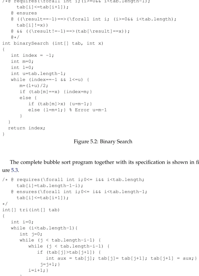
5.3.2 Binary Search . . . 62
5.3.3 Bubble Sort with Initial Condition . . . 63
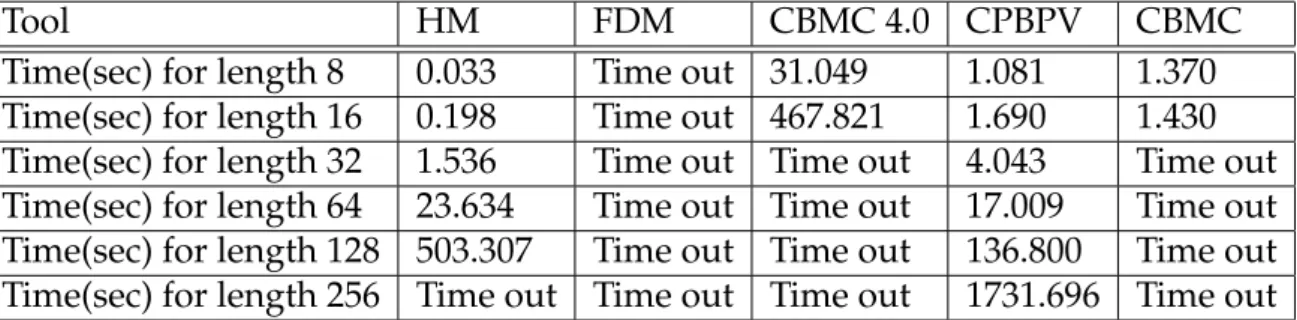
5.4 Comparative Results . . . 65
5.4.1 Triangle Classification . . . 65
5.4.2 Binary Search . . . 66
5.4.3 Bubble Sort . . . 67
6 Conclusions 69 6.1 Summary . . . 69
6.2 Future Work . . . 70
A System of constraints for the benchmark programs 75 A.1 Tritype - Hybrid Model . . . 75
A.2 Tritype - Finite Domain Model . . . 77
A.3 Binary Search - Hybrid Model . . . 78
A.4 Binary Search - Finite Domain Model . . . 80
A.5 Buble Sort - Hybrid Model . . . 81
2.1 A simple one loop program . . . 9
3.1 Subset of Java . . . 30
3.2 Subset of JML . . . 31
3.3 An example program . . . 32
3.4 A sample code illustrating variable versions. . . 34
3.5 Transformation with wrong version of variables . . . 34
3.6 Transformation with correct version of variables . . . 34
3.7 If_Else statement transformation . . . 37
3.8 If_Else statement without the else part . . . 38
3.9 If_Else statement with more changes in the else part . . . 38
3.10 If_Else statement with changes in both of the If and the Else parts . . . . 39
3.11 Transformation of nested If_Else statement . . . 39
3.12 More efficient nested If_Else representation . . . 40
3.13 An example code with a while loop . . . 41
3.14 Constraint system representing a while loop . . . 42
3.15 Sample program with nested while loops . . . 43
3.16 Representation of the inner most loop . . . 44
3.17 Representation of the second inner loop . . . 44
3.18 Constraints’ model corresponding to the sample while loop program . . 45
3.19 Representation of a simple JML specification . . . 47
3.20 Example for transformation of a JML specification with quantifier . . . . 47
3.21 Constraints’ model corresponding to the example program . . . 48
4.1 A finite domain model example . . . 51
4.2 Narrowing of domains to keep bounds consistency . . . 52
4.4 Representation of the example program in the hybrid model . . . 57
5.1 Triangle Classification . . . 63
5.2 Binary Search . . . 64
5.1 triangle classification without an error . . . 65
5.2 triangle classification with an error . . . 66
5.3 binary search without an error . . . 66
5.4 binary search with an error . . . 67
1
Introduction
The continuous reduction in the cost of computing ever since the first days of com-puters has resulted in the ubiquity of computing systems in today’s world; there is no any sphere of life in the daily routine of human beings in the 21st century that is not directly or indirectly influenced by computer systems. Some of the areas where computer systems have become a very important and integral part of their existence include banking, production line control, air traffic control and transportation, etc. But this high reliance of the society on computer systems has not come without a higher risk to today’s society or without a stronger challenge to today’s computer scientists. Since many computer systems of today are safety critical in a sense that failure of such systems can cause a catastrophic loss to the society in terms of not only money and time but also invaluable human life, it is crucial for computer scientists to make sure that computer systems behave correctly under all circumstances. For the whole computer system to behave correctly, it must be ensured that both the hardware and software components behave correctly. However, in this study, we will be interested only in the software component of computer systems, and we deal with techniques of pro-gram verification that are aimed at ensuring the correctness of the software compo-nent. Though most modern computer systems consist of sophisticated hardware and software components, ensuring the correctness of their software component is often more challenging than that of their underlying hardware component.
with constraint solvers playing the role typical verification tools play in typical pro-gram verification set ups. The propro-grams considered are written in some subset of the Java programming language, and their preconditions and postconditions are written in some subset of the Java Modeling Language(JML). The program verification pro-cess has two principal steps: constraint generation and constraint solving. A program together with its precondition and postcondition is first parsed into a system of con-straints. Then, the system of constraints is processed using constraint solvers so that the correctness of the original program is proved to hold, or not, based on the outcome of the constraint solving.
2
Review of the State of the Art
2.1
Introduction
A computer program can be considered as a mathematical object whose properties can be formally specified so that mathematical proofs can be done on the program to check whether the program satisfies a given set of properties or not. Program verification deals with ensuring that programs satisfy the given set of properties. In this work, constraint programming techniques are used for program verification with constraint solvers playing the role typical verification tools would play in typical program verifi-cation set ups.
chapter discusses constraint programming in some detail whose techniques are used for program verification in this work. Section2.3.1provides a formal definition as well as illustration of constraint satisfaction problems (CSPs) followed by a brief coverage of basic constraint solving techniques used by constraint solvers in section2.3.2.
2.2
Program Verification
Program verification is the use of formal techniques to ensure that programs satisfy a set of formally specified correctness properties. As computer programs are becoming part of more and more systems that we depend on for our daily lives, the need for efficient and effective program verification techniques that can be scaled up to industry level programs has been increasing. Most of the methods being commonly practiced today to ensure correctness properties for programs involve simulation of the expected properties of programs, and testing using a set of "critical" test data. There are a few serious limitations to this approach. One limitation is the fact that simulation of today’s complex systems on all possible input sequences in any reasonable time is not possible. Another limitation is the fact that "critical" test data is a very vague expression that lacks formal definition to be of any practical use. Furthermore, whereas simulation and testing methods are very good in detecting well-defined types of errors, they may fail to catch elusive design faults that may make the system to behave unexpectedly only under a particular set of conditions.
In program verification methods, one models a program in a mathematical logic under some well defined theory, and formally proves that the program satisfies its desired specifications. Program verification techniques assume that the input program is syntactically correct - missing semicolons, parenthesis and the like are not the issues of program verification - and their concern will be in detecting semantic difference between the program and its specification.
2.2.1
Correctness of a Program
The correctness of a given program is specified in terms of the desirable properties it needs to satisfy. The main properties used to define correctness of a given program are given below [1]:
1. Partial correctness :
the input should indeed be sorted. It is called partial because the property is defined on the implicit condition of termination; the program is not guaranteed to terminate which means that it is not guaranteed to deliver any result at all in some situations.
2. Termination :
A program is said to terminate if and only if it finishes its computation and ex-its normally or aborts ex-its computation and exex-its abnormally after a finite amount of time. The problem of determining whether a given program will always fin-ish execution or will keep on running forever is called the program termination problem or the uniform halting problem. Although it roots back to the era of Hilbert’s decision problem before the invention of computers, and was proven not to be decidable, the program termination problem was one of the most ac-tively researched and debated areas of theoretical computer science [2].
3. Absence of failures :
Failures in a given program are caused by violations of the operational semantics governing one or more operations in the program or programming language con-structs used in the program. Some common causes of program failures include division by zero, trying to access an array out of its range, and stack overflow. One desirable property of programs is the absence of any such cause of failure.
4. Interference freedom :
It refers to the property that none of the simultaneously running components of a given concurrent program can modify the variables shared with another com-ponent in such a way that the change is undesirable for the other comcom-ponent.
5. Deadlock freedom :
A concurrent program is said to be free from deadlock if and only if it does not end up in a situation where one or more of the non-terminated components of the program are waiting indefinitely for a condition becoming true.
6. Correctness under fairness assumption :
that it will be denied access indefinitely.
The first three properties of correct programs apply for both sequential and concurrent programs whereas the remaining three properties apply only for concurrent programs. In general, ensuring any one of these properties is more challenging for concurrent programs than that of sequential programs. Since this work deals with techniques for verification of partial correctness for a subset of sequential Java programs, this review of the state of the art for program verification will be more focused on approaches to verification of partial correctness for sequential programs.
2.2.2
Earlier Issues in Program Verification
Although formal verification has enjoyed several recent successes in proving correct-ness of industry-scale hardware and software systems, there were mountainous obsta-cles to program verification in its early stage and still there are several objections that are raised against it.
The first challenge is based on the fact that many formal theories are undecidable or they need algorithms with super-exponential time bounds to be decidable. This leads to the conclusion that verification techniques that are based on mechanical theorem proving on such theories may keep on running forever.
The second challenge regards the specification of the desired properties of pro-grams. To verify that a program has a certain property, the property must be speci-fied using some formal language. Here an important question arises: can this formal specification of the program be any simpler than the program itself? If not, verification may end up verifying whether a complicated object representing the program is con-sistent or not, in some complicated technical sense, with another complicated object representing the set of specifications. This can not lead the verification process to cor-rectness and reliability, but instead to a multiplication of the possibility for errors. A more fruitful answer for this challenge was the emergence of specification languages that are solely designed and used for the purpose of clearly specifying the result of computations in programs. These specifications languages are completely different from the programming ones because they are not required to be efficiently executable (or even executable at all).
that 1 is a number, how many will it require to demonstrate a real theorem?" In other words, this comment of suspicion on program verification is based on a questionable view of what, if any, the role of formal methods can be in mathematics and computer science.
2.2.3
Program Verification Methods
Formal verification of programs entails a mathematical proof showing that the pro-gram satisfies its desired set of properties which should be formally specified. This requires some method for mathematically modeling the program and deriving its de-sired set of properties as theorems. The main difference among the various formal verification approaches comes from the choice of the mathematical formalism used in the process of modeling a program and deriving its set of desired properties.
2.2.3.1 1. Program Logics - Hoare Logic
Specifying the semantics of a program in terms of the effects of its instructions on the states of the underlying machine is called an operational approach to modeling the program, and the resulting semantics is called operational semantics [5]. Operational semantics form the basis for program verification using methods such as model check-ing, theorem provcheck-ing, etc. However, the need to reason about the underlying machine in the operational approach makes it cumbersome to prove correctness of a program. Program logics on the other hand focus on simplifying program verification by factor-ing out the details of the machine executfactor-ing the program from the verification process. The goal in program logics is to deal with the program text itself as a mathematical object [6,7].
In program logics, each instruction of the program is considered as performing a transformation of predicates. For some sequence of instructionsI in a given program-ming language, the axiomatic semantics of the programprogram-ming language are specified by a collection of formulas of the form{P}I{Q}, whereP and Q are first order pred-icates over the program variables. Such a formula can be read as: "IfP holds for the state of the machine when the program is poised to executeI, then, after the execution ofI, Qholds." Predicates Pand Qare called the precondition and postcondition for I respectively.
For example, ifI is a single instruction specifying an assignment statement x:=a, then its axiomatic semantics is given by the following schema, also known as the Axiom o f Assignment.
{P}x:=a{Q}holds ifQis obtained by replacing every occurrence of the variablexinP bya.
Hoare [103] provides five such schema, and an inference rule often calledrule o f composition to specify the semantics of a simple programming language.
Rule of Composition:
Infer{P}hi1:i2i{Q}from{P}i1{R}and{R}i2{Q}. Herehi1:i2irepresents the sequential
execution of the instructionsi1andi2. Another rule that allows generalization and use
of logical implication is given below. Rule of Implication:
Infer{P}i{Q}from{R1}i{R2},P =⇒ R1, andR2 =⇒ Q.
Hoare logic, which is an instance of program logics, is defined as a proof system that consists of first-order logic, together with Hoare axioms and inference rules to deal with program correctness. In order to use Hoare logic to reason about program cor-rectness, assertions need to be mapped to predicates on the program variables, and instructions of the program are considered as transformation of such predicates. The semantics of a programming language specified by describing the effect of executing instructions on assertions about states (rather than states themselves) is known as ax-iomatic semantics. Hoare logic (or in general program logics) is a proof system over the axiomatic semantics of the programming language. GivenPand Qas the precon-dition and postconprecon-dition of the program Π respectively, proving correctness consists of deriving the formula{P}Π{Q}as a theorem.
To do program verification, one annotates the program with assertions at certain loca-tions that corresponds to the entry and exit of the basic blocks of the program such as loop tests, and the entry and exit points of the program itself. These annotated pro-gram points are called cutpoints. The entry point of the propro-gram is annotated with the precondition, and the exit point is annotated with the postcondition. One then shows that if the program control is in an annotated state satisfying the corresponding asser-tion, then the next annotated state will also satisfy its assertion.
Let us consider the simple one loop program in figure2.1: it has 2 variables X and Y, and loops 5 times incrementing X and decrementing Y in each iteration. The cutpoints for the program are at counters 1 (program entry), 3 (loop test), and 7 (termination). The assertions associated with each cutpoint are shown to the right. The precondition Pis assumed to be universally true, and the postcondition says that the variable X has the value 5.
1. X:=0; {T} 2. Y:=5;
3. if (Y<1) goto 7; {(X+Y)=5} 4. X:=X+1;
5. Y:=Y-1; 6. goto 3;
7. HALT {X=5}
Figure 2.1: A simple one loop program
3. To show that given the assertion at 1, after executing counters 1 and 2, the asser-tion at 3 holds (which can be represented as 1→ 3), we need to prove the formula {T}hX :=0;Y :=5i{(X+Y) =5} as a theorem. The formula is called proof obligation. By applying the axioms of assignment, rule of composition, and implication rule, the simplified proof obligationT =⇒ (0+10) =10is obtained. From this example, it can be seen that by applying Hoare axioms, a formula that is free from constructs of the pro-gramming language is obtained. Such a formula is called verification condition. The complete correctness proof of the program given above consists of generating such ver-ification conditions for each of the execution paths 1→3, 3→3, and 3→7, and showing they are logical truths. In practice, the verification conditions can be more complicated formulas with a need to do non-trivial proofs.
Doing program verification using axiomatic semantics requires two tools:
• a verification condition generator(VCG) that takes an annotated program as an input and generates the verification conditions
• a theorem prover that proves the verification conditions
A possible pitfall of this approach is the fact that it depends on two trusted tools, namely a VCG and a theorem prover. Nevertheless, program logics and axiomatic semantics have been commonly used both in program verification theory and its ap-plication [8,9,10]. The principal benefit of using this approach is to abstract out details of the underlying machine from the program.
2.2.3.2 2. Theorem Proving
be interpreted as self-evident truths about the object, and a set of validity preserving inference rules for deriving new formulas about the object from the existing ones. The logic has to make sure that the set of formulas representing axioms are valid, and the set of inference rules are validity preserving which means that the application of one or more inference rules of the logic to the axioms must result in a valid formula. A formula resulting from applying one or more inference rules to the axioms of the logic is called a theorem. A sequence of one or more formulas such that each formula is either an axiom or result of applying an inference rule to some other formula that come before this formula in the sequence is called a derivation or deduction. In the sense of theorem proving, verification means the process of showing the existence of at least one derivation for some formula of interest in the logic of the theorem prover.
Being the base for the theorem proving approach, there has been a number of the-orem provers being in use today. Some of the most popular ones include HOL, Coq, ACL, Isabelle, NuPrl, PVS, TPS and Leo. The logics these theorem provers are designed to work with range among various domains; there are theorem provers for first-order logic, higher-order logic, set theory, etc. There are also significant variations among theorem provers depending on the level of automation and the need of interaction with a user. Some like HOL needs more interaction with trained users while others like PVS can work fine with just a little need of interaction with the user. Theorem provers like TPS and Leo require no interaction with a trained user and hence belong to a group of theorem provers called Automatic Theorem Provers (ATPs). Despite these diversity of features, one common feature of all theorem provers is that they support logics that are very expressive. This expressivity has allowed the applications of theorem provers to proof well known theorems in different mathematical domains. The best example is that Nqthm theorem prover has been able to mechanically verify Godel’s incomplete-ness theorem [11]. But, this expressivity does not come without a cost; as it was pointed out in section2.2.2, any such sufficiently expressive logic that is consistent must be un-decidable. This means that there can not be an automatic procedure for determining if there is a derivation for some formula in a given logic, and therefore, the successful use of theorem proving for deriving nontrivial theorems typically requires interaction with a trained user. Any attempt to do theorem proving without a need of interaction between the theorem prover and the trained user requires trading of expressivity for automation like the case for the ATPs.
Nevertheless, theorem provers remain as one of the most important players in the area of formal verification. Three of the most important things theorem provers are generally known to do are:
sequence of formulas corresponds to a valid derivation in the formal logic. This is done by checking if each formula in the derivation is either an axiom in the formal logic or a result of applying an inference rule from the formal logic on the previous formula of the sequence.
• When a heuristics for proof search is provided by the user, the theorem prover can practically assist the user in the construction of a proof by implementing the heuristics. Such heuristics of proof search include generalizing the formula for applying mathematical induction, using appropriate instantiation of previously proven theorems, judicious application of term rewriting, and so on.
• If the formula to be verified as a theorem can be expressed in some well-identified decidable subset of the formal logic, then the theorem prover can make use of decision procedures to determine if the formula is a theorem or not without a need to interact with a trained user. For example, the ACL2 theorem prover that has decision procedures for deciding linear inequalities over rationals [12]. Although there have been major successes in approaches aimed at automating the search of proofs, undecidability still poses strong challenge on the automation. There-fore, having a substantial interaction between the theorem prover and a trained user is inevitable during the construction of nontrivial derivation for a formula using theo-rem proving. In the interaction, the user is responsible for providing an outline for the derivation of the formula required to be proved, and the theorem prover is responsi-ble for deciding if a formal proof can be devised from the outline that can be used for deriving the formula.
The approach to verify correctness of programs using theorem provers is exactly the same as the approach to prove the correctness of any other mathematical statement in a formal logic. The desired properties of the program are specified as formulas in the logic of the theorem prover, and an attempt to derive the formulas is made from the logic using the inference rules of the logic. But the size of the formulas that need to be manipulated in order to verify programs could be extremely larger than those manipulated to prove typical mathematical statements.
The main goal in formal verification research has been to automate proofs of cor-rectness as much as possible which does not match with the fact that theorem provers in practice need interaction with trained users to perform their activities. Neverthe-less, theorem provers continue to be very useful players in formal verification for the following 3 important reasons:
one can depend on for proving such properties.
• Sometimes even when specifying the desired correctness properties is possible with some decidable logic, for example, when one wants to reason about a finite-state system, theorem proving has the advantage of being both succinct and gen-eral.
• A very practical reason to use theorem proving is that fact that theorem provers provide a substantial degree of control of the derivation process of complex theo-rems for the user. This can be exploited by the user in different ways, for example, by proving key intermediate lemmas that assist the theorem prover in its proof search.
2.2.3.3 3. Model Checking and Bounded Model Checking
In theorem proving, automation is traded for the expressivity of the formal logic used in the given theorem prover. But this does not change the fact that automation is the ultimate target of formal verification, whether for a program or a more complex com-puting system, and therefore, enabling automated verification, if possible, is a key con-sideration. Given a desirable property to be verified, automated verification methods make use of a decidable formalisms to represent the property as a formula under the formalism being used, and a decision procedure, an algorithm that terminates with the correct yes/no answer for some given decision problem, to prove the truth or falsity of the formula.
by the reachable states of the program by exhaustively exploring each of these states. If the desired property holds in all states of the program, the algorithm terminates with the answer true; otherwise if it does not hold in any of the reachable states of the pro-gram, the model checking algorithm computes a counterexample, an execution trace leading to a state of the program in which the property does not hold. This procedure is guaranteed to terminate if the state space is finite. The ability of model checking algorithms to compute counterexamples is considered as a key feature, and by some even as a reason for its acceptance as a formal verification techniques [15]. Although the direct application of model checking techniques to implementation level code can significantly increase the computational requirements for a verification, the promise of this approach is that it can eliminate the need for expert model builders and can place the power of automated verification techniques where it belongs: in the hands of programmers [16].
Model checking tools verify partial specifications that are usually classified as safety or liveness properties. Safety properties describe the unreachability of bad states, such as when null pointer is dereferenced, stack overflow has occurred, API usage con-tracts, like the order of function calls, are not respected, etc. Liveness properties on the other hand describe that something good eventually happens such as the condi-tion that requests must be served eventually, a program must eventually terminate, etc. Like program logics, model checkers take specifications of a program given in the form of preconditions and postconditions. However, unlike the case in program logics where different specifications are given for the properties that should hold at differ-ent points in the program, specifications in model checkers are defined for the differ-entire program.
The fact that model checking algorithms are based on exhaustive examination of reachable states has raised a very critical issue in model checking called state-space explosion: the state-space of a program is exponential on various parameters of the program of which the most important ones are number of variables and the width of the data-types. The state-space can even be infinite if there exist function calls and dynamic memory allocations in the program. Concurrency worsens the problem even more due to the different thread schedules that must be considered which are expo-nential on the number of statements in the program. Despite the possibility of ending in unmanageably huge state-space, model checking algorithms generate sets of states to be analyzed by using instructions in the program, and store them to ensure that they are visited no more than once.
Symbolic model checking algorithms. Explicit-state model checking algorithms use an explicit representation of the system’s global state graph, usually given by a state tran-sition function. Symbolic model checking algorithms use a symbolic representation for the state set, usually based on binary decision diagrams [17].
Explicit state model checking methods need to explicitly represent the program as a state transition graph by recursively generating successors of states starting from the initial state. The graph may be constructed in a depth-first, breadth-first, or using some heuristic. Every time a new state is generated, it is checked for a property violation on the fly, so that errors can be detected without a need to build the entire graph. Explored states are stored in a hash table to avoid recomputing their successors when some state that has been already explored is regenerated. The generated states are compressed before storage so that memory usage is optimized. If the available memory is insuffi-cient, lossy compression methods can be used. This may be risky because it may lead to some error states being missed. In practice, with state spaces containing close to a billion states, and hash tables of several hundred megabytes, the probability of miss-ing a state can be less than 0.1% [18]. An important method of pruning state space exploration for concurrent programs is called partial order reduction [19]. The order in which instructions in different threads are executed may not make a difference for proving some properties. Transitions whose interleavings do not affect the property can be grouped into classes. A model checker only needs to generate one represen-tative of each class while constructing the state graph. In the best case, partial order reduction can reduce the state space to be explored by a factor that grows exponen-tially in the number of threads. An explicit state model checker evaluates the validity of the temporal properties over the model by interpreting its global state transition graph as a Kripke structure, and property validation amounts to a partial or complete exploration of the state space.
space are comparable with that of BDDs for finite state space [23]. Symbolic represen-tations such as propositional logic formulas are more memory efficient, at the cost of computation time.
Symbolic techniques work well for proving correctness and handling state-space explosion due to program variables and data types. Explicit state techniques are well suited to error detection and handling concurrency. A general approach to counter the issue of state-space explosion that is not specific to proving correctness or detecting errors unlike the two techniques above is abstraction. Since a program can, in general, be represented by an infinite-state model, existing tools do not directly check programs against specifications. Instead, a conservative finite state abstraction of the program is first generated. In this approach, the state-space explosion is prevented by analyzing a sound abstraction of the program that consists of smaller state space. Such an ab-straction of the program used to be manually constructed, but due to advancements in the corresponding tools recently, the construction can now be done automatically. A framework known as CounterExample Guided Abstraction Refinement (CEGAR) [24] iteratively create a more precise abstractions of the program until the desired proper-ties are proven or a real counterexample is generated. Chaki, et al. [24] summarizes the CEGAR process as follows:
• Model Creation : A model is computed using the control flow graph (CFG) of the program in combination with an abstraction method called predicate abstraction [25], [26]. Properties such as the equivalence of predicates are decided with the help of a theorem prover.
• Verification : Verify that the abstraction conforms to the specification. If this is the case, the verification is successful. Otherwise, obtain a possibly spurious coun-terexample and go to the next step
• Validation: Check whether the counterexample extracted in the verification step is valid. If this is the case, then we have found an actual bug and the verification terminates unsuccessfully. Otherwise construct an explanation for the spurious-ness of the counterexample and proceed to the next step
The explicit state, symbolic as well as abstraction based model checking approaches discussed above differ from each other on how they view and try to tackle the state-space explosion. But in general, there are two approaches to program verification using model checking. The first approach requires transforming the implementation level specification of the program (the code) systematically into a language that some given verification tool can recognize. The program is rewritten in the syntax of the given verification tool. An example is the first Java Pathfinder [27] which targets the SPIN model checker [28]. This approach requires building a sort of parser that can read and transform the implementation level specifications of the program (the actual code) into detailed verification models that can be verified by a model checker. For the trans-formation to be done accurately, the parser needs to be able to interpret the semantic content of the program, and transform it into equivalent representations in the verifi-cation model. The second approach involves the design of verifiverifi-cation tools that can take the program written in a certain programming language, and do the verification reasoning on the program itself without a need for transformation. The verification tool is designed specifically to handle a given programming language, and separate tools are needed to handle each and every language. Examples for this approach in-clude the second Java Pathfinder tool [29] and Blast tool [30]. This approach requires a verifier that can make accurate decisions on the validity of a program execution af-ter reasoning on the program itself. The major challenge in this approach will be the construction of a full fledged verification tool for any formally defined programming language. The challenge will be exacerbated for a programming language that was not designed initially with the intention of making it amenable for verification tools.
In conclusion, the following facts have paved the way for the acceptance and high success of model checking techniques in formal verifications of computing systems:
• Model checking is automatic
• Its approaches are not mainly based on doing proofs
• Model checking algorithms run fast
• When verification fails, counterexamples are generated, and
• It works well with Partial specifications
as discussed earlier in this section. The integration of abstraction techniques into this process attracted a range of interest in model checking from the industry. This was fol-lowed by a significant number of realistic systems, mostly of hardware nature, could be verified using these model checking methods, which eventually resulted in accep-tance and adoption of the methods in various areas of the computing industry in gen-eral. The principal limitation of these methods is the large memory requirement of the boolean functions used to represent the set of states. This limitation had motivated Biere et al. to propose a technique called Bounded Model Checking(BMC) in 1999 [21] which was based on SAT techniques rather than BBDs. This technique is a form of Model Checking that performs a depth-bound exploration of the state-space which im-plies that the need to examine the entire state space is relaxed. BMC explores program behavior exhaustively, but only up to a certain depth limit. If the incorrect properties of the program are exhibited only in states that are beyond this depth limit, then BMC will not catch this bugs, and may "verify" the program as correct.
Therefore, it is important of the BMC algorithm to explore "deep enough" so that there is a guarantee that all the behaviors of the program are represented and evalu-ated, and exploring further deep will only get states that have already been explored. The depth limit that provides such a guarantee for the BMC algorithm is called a com-pleteness threshold [31]. However, since finding the smallest such threshold is as hard as model checking itself, in practice, BMC based methods usually try to compute and make use of an approximate value for the completeness threshold. The approxima-tion can be done either through syntactic analysis or by using iterative algorithms. The first option uses the high-level worst-case execution time (WCET) to approximate the depth-bound. Since this time is given by a bound on the maximum number of loop-iterations, the number of loop-iterations is computed first by simply using syn-tactic analysis of the loop structures, and then the WCET time is determined from the number of loop iterations. If the number of loops can not be extracted from the loop structures, iterative algorithms will be applied to approximate the bound. In the iterative algorithm approach, an initial guess of the bound on the number of loop it-erations is made, and then the loop is unrolled up to the bound with the assumption that some conditions called unwinding assertions hold. If the conditions are violated, a new higher bound is guessed, and the algorithm proceeds recursively until it reaches a point where the unwinding assertions are satisfied. This method is very useful when loops in a given program have run-time bound.
side, BMC is not generally complete, and completeness can be guaranteed only for programs whose loops are not too deep.
There are a number of tools that implement BMC for program verification. BMC was applied for the first time as a novel formal verification approach for equivalence checking of small, assembly-language routines for digital signal processors (DSP) by Currie et al. [32]. One of its first implementations of BMC for C programs is CBMC [33] developed at Carnegie Mellon University.
In this work, constraint programming techniques are applied to the bounded model checking approach to get an efficient program verification framework. Therefore, we will first discuss the main features of constraint programming in the next subsection.
2.3
Constraint Programming
Constraint programming is one of the most exciting developments in programming languages of the last two decades. It has now become one of the most suitable meth-ods for modeling and solving optimization problems that involve complex relation-ship among entities of the problem, and combinatorial search. This is due to the fact that constraint programming is based on strong theoretical foundation. Unlike tra-ditional programming languages, for instance object oriented languages, that provide little support for specifying relationships among the programmer defined objects, such relationships among programmer-defined objects form the base of constraint program-ming. This fact is attracting widespread commercial interests as many critical problems like job scheduling, timetabling and routing can be efficiently solved using constraint programming.
A constraint is a restriction on the space of possibilities for some choice; it can be considered as a piece of knowledge that filters out the options that are not legitimate to be chosen, and hence narrowing down the size of the space. Formulating problems in terms of constraints has proven useful for modeling fundamental cognitive activities such as vision, language comprehension, default reasoning, diagnosis, scheduling, and temporal and spatial reasoning, as well as having applications for engineering tasks, biological modeling, and electronic commerce [34].
2.3.1
Constraint Satisfaction Problem(CSP)
A CSP in general consists of three main components:
• A set of domainsfor each variable in the CSP. The set of possible value for each variable is called its domain.
• A set of constraints which are rules that impose limitation on the values that a variable or a combination of variables may be assigned.
Therefore, a CSP can be defined as a model of some problem that consists of variables, their domains, and constraints. A common example to illustrate a CSP is then−Queens problem which is aimed at placingnqueens on ann×nchessboard such that there is no possibility of attack between any two of thenqueens. Two queens are said to attack each other if they are put on the same row or the same column or the same diagonal of the chessboard. One way of modeling this problem as a CSP is as follow: there aren variables{x1, ...,xn}for each column of the chessboard, the domains for each variablexi
will beDi={1, ...,n}, and the constraint on each pair of columns is that the two queens must not share a row or a diagonal.
Formally, a CSP can be defined as the triplehX,D,Ci, whereX is a finite set of vari-ablesX ={x1, ...,xn}, with respective domainsD={D1, ...,Dn} which list the possible
values for each variableDi={v1, ...,vk}, and a set of constraintsC={C1, ...,Ct}. A
con-straintCi can be viewed as a relation Ri defined on the set of variables Si ⊆X such thatRi denotes the simultaneous legal value assignments of all variables in Si. Thus, the constraintCi can be formally defined as the pair hSi,Rii; Si is called the scope of the constraint. A solution of the CSP is an n-tuplehV1, ...,Vniwhere eachVi∈Di
corre-sponds to the value assigned to each variablexi∈X, and the assignment satisfies all constraints inCsimultaneously.
For example, the n−Queen problem for the case of 4 queens can be modeled as a CSP using finite domains as follows: There are four variablesX ={x1,x2,x3,x4}, with
domainDi={1,2,3,4}for each of the variables. There are six constraints that avoids any two queens from attacking each other; C1=R1,2, C2 =R1,3, C3 =R1,4, C4= R2,3,
C5=R2,4, andC6=R3,4. Here, Ri,j is a relation mapping each possible value of queen iwith a possible value of queen jsimultaneously. The six constraints are given below by extension:
• R1,2= {(1,3),(1,4),(2,4),(3,1),(4,1),(4,2)}
• R1,3= {(1,2),(1,4),(2,1),(2,3),(3,2),(3,4),(4,1),(4,3)}
• R1,4= {(1,2),(1,3),(2,1),(2,3),(2,4),(3,1),(3,2),(3,4),(4,2),(4,3)}
• R2,3= {(1,3),(1,4),(2,4),(3,1),(4,1),(4,2)}
• R3,4= {(1,3),(1,4),(2,4),(3,1),(4,1),(4,2)}
Constraint programming is enabled by embedding constraints in some host lan-guage. The first host languages used were logic programming languages such as Pro-log, which explains the reason for the field to be initially called constraint logic pro-gramming. In the language of Prolog, the domains of variables were represented as a set of Herbrand terms and constraints were formed as equalities between Herbrand terms. A CSP that consist of such constraints is solved by using the unification facility of the Prolog host language to unify the Herbrand terms. For example, the constraint stud(Id,Name) =stud(35031,tewodros)is solved through unification by assigning Id to 35031 and Name to tewodros. Constraint logic programming has been extended to constraints over other domains among which the most important ones are boolean constraints, real linear constraints and finite domain constraints.
2.3.1.1 Boolean Constraints
A constraint is called boolean if each variable in the constraint has a domainD={0,1}. Such constraints are particularly useful for modeling digital circuits, and boolean con-straint solver can be used for verification, design, optimization etc. of such circuits.
2.3.1.2 Finite Domain Constraints
All variables in such constraints get associated with some finite domain, either explic-itly declared by the program, or implicexplic-itly imposed by the finite-domain constraint solver. By finite domain, we mean any set that can be mapped into a subset of integers. Therefore, only integers and domain variables are allowed in finite domain constraints. Finite-domain constraint solvers mainly deal with two classes of constraints called primitive constraints and global constraints. All other types of constraints are automat-ically translated to conjunctions of primitive and global constraints, and then solved. Classes of primitive constraints defined by the solver include:
• Membership constraints: Examples includeX in1..5which constraints the vari-ableX to have the set{1,2,3,4,5} as its domain, anddomain(L,1,5)which con-straints a list of variablesL such that each variables inLhas the set {1,2,3,4,5} as its domain.
• Reified constraints: Instead of merely posting constraints, it is often useful to reflect its truth value into a boolean variable B, so that the constraint is posted if B is set to 1, the negation of the constraint is posted if B is set to 0, B is set to 1 if the constraint becomes entailed, and B is set to 0 if the constraint becomes disentailed. This mechanism is known as reification. A reified constraint is writ-ten asCons#<=>BwhereConsis the constraint to be reified andBis a boolean variable.
• Propositional constraints: are complex constraints formed by combining indi-vidual constraints using propositional combinators. The main propositional com-binators include #/\, #\/, #=>, and #<=> which play roles similar to logical conjunction, disjunction, implication and bi-implication respectively. For exam-ple, given constraintsC1 andC2, the propositional constraintC1#/\C2 (C1#\/C2)
is satisfied if and only if both(either) ofC1andC2are satisfied.
Another propositional constraintC1#=>C2valuates to true ifC1is false orC2is
true. An important property of this constraint is that ifC1is true (resp.C2is false),
thenC2should necessarily be true (resp.C1should necessarily be false). This can
be used to specify constraints that are needed only under some condition. For this reason, such constraints are also called conditional constraints.
Some of the most important global(combinatorial) constraints defined by the solver include all_different, element, global_cardinality, etc. For example,all_di f f erent([X,Y,Z])
constraints any variable in the list to take a unique value which is different from any other variable in the list. Another global constraint,element(X,L,Y), constraintsY to be theXth element of the listLgiven some listL.
New user-defined primitive constraints can be added to the solver by writing so-called indexicals whereas new user-defined global constraints can be also written in Sicstus Prolog by means of a programming interface. A detailed explanation of the various finite-domain constraints defined by the solver together with how to add user defined constraints is given in [35].
2.3.1.3 Real Linear Constraints
the lazy treatment of nonlinear equations, to feature a decision algorithm for linear in-equalities that detects implied equations, to remove redundancies, to perform projec-tions (quantifier elimination), to allow for linear dis-equaprojec-tions, and to provide linear optimization [35].
2.3.2
Constraint Solving Approaches
Given a CSP hX,D,Ci, there are different ways of getting a value for each variable in X from its respective domain in D that satisfies all constraints in C. A framework that has utilities defined in it for modeling a given problem as a CSP, and that produces the solution to the CSP if there is at least one or that tells the absence of a solution is called a constraint solver. There are two broad classes of constraint solvers: complete solvers and incomplete solvers.
2.3.2.1 Complete Solvers
Complete solvers implement decision procedures that take a given CSP and produces a solved form of the problem. Examples of complete solvers include CLP(R) and CLP(B) that are used for solving real linear constraints and boolean constraints respectively. Although solving real linear constraints in itself is not possible in polynomial time, since CLP(R) implements simplex algorithms, solving linear constraints is quite ef-ficient. However, for CLP(B), the fact that the underlying representation of boolean functions is based on Boolean Decision Diagrams results in exponential time being required for solving constraints.
2.3.2.2 Incomplete Solvers
any solution. Example includes CLP(FD) which is used to solve constraints over finite domains. Boolean constraints can also modeled here as special case of finite domain constraints with each variable having the domainD={0,1}. Since propagation may be of no use in the worst case scenario, eventhough propagation has a polynomial time complexity, the CLP(FD) solver has an exponential time complexity on the size of the domains.
There are different levels of consistency criteria that can be achieved by the con-straint propagation algorithm. The most important ones include node consistency, arc consistency, and bound consistency.
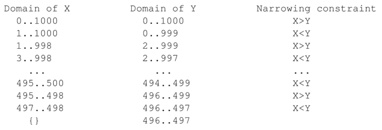
A CSP is node-consistent if there does not exist a value in the domain of any one of its variables that violates a unary constraint in the CSP. This criterion is of course very trivial but it is very important when it is considered in the context of an execution model that incrementally computes solution from partial solutions.A more demanding consistency criterion is arc-consistency. To be considered for arc-consistency, a CSP must first be node-consistent. In addition, for every pair of variableshX,Yi, for every constraintCxy defined over variablesX andY, and for each valueVx in the domain of X, there must exist some valueVyin the domain ofY that supportsVx. For example, the CSPh{X,Y},{1..5,1..5},{X+Y >7}i is not arc-consistent because there is no support in the domain ofY when X takes 1 or 2 that satisfies the constraint X+Y >7. The same holds forY also. An arc-consistent CSP which is equivalent to the original CSP is obtained by reducing domains of X and Y from{1,2,3,4,5}to{3,4,5}.
Another type of consistency criteria is called bounds consistency defined on nu-meric constraints which are arithmetic constraints of equalities or inequalities. For ex-ample, the CSPh{X,Y},{1..10,1..10},{X >Y}i in not bound-consistent because there are some bound values in the domain of both variables that can never be part of any so-lution as they do not have any matching value in the other variable to satisfy the given constraint. If X takes the value 1, then there is no any matching value in Y that can sat-isfy the constraintX>Y. Therefore 1 should not be in the domain of X. Similarly, there is no matching value for X when Y takes the value 10. Likewise, 10 should not be in the domain of Y. A bound-consistent equivalent CSP will beh{X,Y},{2..10,1..9},{X>Y}i. Another example can be the CSPh{X,Y},{3..10,1..8},{X=Y}i. There is no any match-ing values for Y when X takes either of 9 or 10 because we have an equality constraint X =Y. Similarly should Y take either 1 or 2, there is no matching value in X that satisfies the given constraint. A bound-consistent equivalent CSP in this case will be h{X,Y},{3..8,3..8},{X =Y}i.
3
Constraints Model Generation
In this work, an efficient way of verifying a program with respect to its specification is studied. The input program is written in some subset of Java, and its specifica-tions (precondition and postcondition) are written in some subset of JML. The only datatypes allowed in the program are integers and array of integers. The program is assumed to be functional and sequential, and it is assumed not to make any func-tion calling. The desired property of the program we are interested to prove is partial correctness with respect to the its specification.
3.1
Introduction
For the verification of a given program via constraints programming as a tool, there must be a way of transforming the original program into a system of constraints on which the actual verification process can be done using constraint solvers. The success of the verification process depends not only on how efficiently the solver can solve the constrains system but also on how accurately the original program can be trans-formed into the system of constraint. The accuracy of the transformation is very crucial because a significant difference between the original program and the corresponding system of constraints will make any judgment that has been made about the original program based on the system of constraints unacceptable. Therefore, the transforma-tion should always keep the semantics and logic of the original program, and the only significant difference allowed is the representation used. In this study, the original program is written in Java and its corresponding constraint system uses Sicstus Prolog syntax. The responsibility of keeping the semantics and logic of the original program in the resulting system of constraints falls on the parser which is the component doing the task of transforming the Java program into a constraint logic program in Sicstus Prolog.
3.2
The subset of Java language handled
The original program which is the input to the parser can be considered as consisting of two main parts; the first part is the specification of the preconditions and postcondi-tions of the program written in JML, and the second part is the actual program written in Java. Although the parser does the translation of both parts together, the languages used to program or specify these two parts are totally different, and the subsets of each of these languages that the parser can handle are also different. Therefore, the parser considers the original program as a JML code, which specifies the preconditions and postconditions of the program, followed by the actual Java program as shown in the grammar below.
Original_Program --> JML_Code, Program
3.2.1
Subset of Java language
The subset of Java language the parser can handle contains only basic and simple struc-tures of the language that are sufficient to handle the sample programs used in this study but the subset can be scaled up in case of any need to incorporate more struc-tures.
The parser assumes the input program to be a function that has a return type, a name which is an identifier, a list of arguments which are the input parameters of the func-tion, and contains a code block followed by a return statement between opening and closing parentheses.
Program --> Type, Identifier, ’(’,List_Of_Arguments,’)’,
’{’, Code_Block, Return_Statement, ’}’
A code block is a sequence of statements where each statement can be a declaration, an assignment, an if_else statement, a while loop or any of these followed by a code block.
Code_Block --> Declaration | Declaration, ’;’, Code_Block |
Assignment | Assignment, ’;’, Code_Block |
If_Else | If_Else, Code_Block |
WhileLoop | WhileLoop, Code_Block
consists of the equality sign=, and an identifier and an expression to the left and right hand side of the sign respectively.
Type --> int | int,’[’, ’]’
Declaration --> Type, Identifier
Assignment --> Identifier, ’=’, Expression
The definition of an expression is given recursively as a number, an identifier, or any two expressions combined by one of the arithmetic operators in {+,−,∗, /}. In Java, an array variable of type integer can have additional expressions for different purpose; for example given an array variablearr, itsith element can be given as the expression arr[i], and its length can be given as the expressionarr.length. Since this two types of expressions are used repeatedly in the sample programs considered in this study, it has been inevitable for the parser to include them in the base definition of expressions, in addition to numbers and identifiers. The full definition of an expression is given below.
Expression --> Number | Identifier |
Identifier, ’.’, length |
Identifier, ’[’, Expression, ’]’ |
Expression Binary_Op Expression
Binary_Op --> ’+’ | ’-’ | ’*’ | ’/’
An if_else statement consists of the keywordi f followed by a condition, a code block in between two parentheses and an optional else part. The else part starts by the keyword elsefollowed by a code block in between two parentheses.
If_Else --> if, Condition, ’{’, Code_Block, ’}’ |
if, Condition, ’{’, Code_Block, ’}’, else,
’{’, Code_Block, ’}’
A while-loop is a statement that starts with the keywordwhilefollowed by a condition and a code-block in between two parentheses.
WhileLoop --> while, Condition, ’{’, Code_Block, ’}’
A condition is a unit-condition, negation of another condition or any two conditions combined using a boolean operator. A unit-condition consists of two expressions com-bined together by a comparison operator.
Condition --> UnitCondition | ’!’, Condition |
UnitCondition --> Expression, Comparison_Op, Expression
Comparison_Op --> ’==’ | ’!=’ | ’>’ | ’>=’ | ’<’ | ’<=’
Boolean_Op --> ’&&’ | ’||’
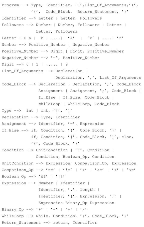
The complete grammar for the subset of Java language the parser can handle is shown in figure 3.1. In addition to the main structures whose definition is given above, the grammar below contains definitions of basic structures like Identi f ier, Number and Return_Statementthat are used as the building blocks in the definitions above.
3.2.2
Subset of JML
Like the subset of the Java language considered above, the subset of JML that can be handled by the parser contains only basic structures of the modeling language that are used in the sample programs considered in this study. In case of any need to handle more structures, the subset can be extended by providing the definitions of the addi-tional structures to the parser.
A JML code consists of the precondition followed by the postcondition.
JML_Code --> ’/*’, Precondition, Postcondition,’*/’
A precondition starts by the character@followed by the keywordrequires, and then a JML-condition will complete the definition.
Precondition --> ’@’, requires, JMLCondition
A postcondition has the character @ and the keyword ensures at the beginning fol-lowed by a postcondition block. A postcondition block is defined as a sequence of one or more postcondition statements. Each postcondition statement starts by the character @followed by two JML-conditions which are separated by the symbol==>showing the implication relation between the two conditions.
Postcondition --> ’@’, ensures, Postcondition_Block
Postcondition_Block --> Postcondition_Statement |
Postcondition_Statement, ’&&’,
Postcondition_Block
Postcondition_Statement --> ’@’, JMLCondition, ’==>’, JMLCondition
Program --> Type, Identifier, ’(’,List_Of_Arguments,’)’, ’{’, Code_Block, Return_Statement, ’}’ Identifier --> Letter | Letter, Followers
Followers --> Number | Number, Followers | Letter | Letter, Followers
Letter --> a | b | ....| ’A’ | ’B’ | ....| ’Z’ Number --> Positive_Number | Negative_Number
Positive_Number --> Digit | Digit, Positive_Number Negative_Number --> ’-’, Positive_Number
Digit --> 0 | 1 | ... | 9
List_Of_Arguments --> Declaration |
Declaration, ’,’, List_Of_Arguments Code_Block --> Declaration | Declaration, ’;’, Code_Block |
Assignment | Assignment, ’;’, Code_Block | If_Else | If_Else, Code_Block |
WhileLoop | WhileLoop, Code_Block Type --> int | int, ’[’, ’]’
Declaration --> Type, Identifier
Assignment --> Identifier, ’=’, Expression
If_Else --> if, Condition, ’{’, Code_Block, ’}’ | if, Condition, ’{’, Code_Block, ’}’, else, ’{’, Code_Block, ’}’
Condition --> UnitCondition | ’!’, Condition | Condition, Boolean_Op, Condition
UnitCondition --> Expression, Comparison_Op, Expression Comparison_Op --> ’==’ | ’!=’ | ’>’ | ’>=’ | ’<’ | ’<=’ Boolean_Op --> ’&&’ | ’||’
Expression --> Number | Identifier | Identifier, ’.’, length |
Identifier, ’[’, Expression, ’]’ | Expression Binary_Op Expression Binary_Op --> ’+’ | ’-’ | ’*’ | ’/’
WhileLoop --> while, Condition, ’{’, Code_Block, ’}’ Return_Statement --> return, Identifier
JMLCondition --> Condition |
forall, Declaration, ’(’,Condition, ’&&’,
Condition, ’)’, ’;’, Condition
The complete grammar for the subset of JML the parser can handle is shown in fig3.2.
JML_Code --> ’/*’, Precondition, Postcondition, ’*/’ Precondition --> ’@’, requires, JMLCondition
JMLCondition --> Condition |
forall, Declaration, ’(’, Condition, ’&&’, Condition, ’)’, ’;’, Condition
Postcondition --> ’@’, ensures, Postcondition_Block Postcondition_Block --> Postcondition_Statement |
Postcondition_Statement, ’&&’, Postcondition_Block
Postcondition_Statement --> ’@’, JMLCondition, ’==>’, JMLCondition
Figure 3.2: Subset of JML
3.2.3
An example program
The program below computes the sum of all even numbers less than or equal to a given integer number. The program requires its input not to be a negative number and in turn it ensures its output to have some value depending on the value of the input and whether this input is even or odd. The program along with its precondition and postconditions written in the subset of Java language and JML subset the parser is made to recognize is shown in figure3.3.
Therefore, in order for some program to be transformed into the constraint system using the constraint solvers that can do the verification process, the program must be written using only the constructs and syntax that can be recognized by the parser.
3.3
Input program to constraints model transformation
3.3.1
An important consideration: versioning
/*@ requires (N>=0);
@ ensures @ (N mod 2== 0)==>(/result==(((N*N)+(2*N))/4)) && @ (N mod 2==1)==>(/result==(((N*N)-1)/4))
*/
int sumOfEven(int N) { int i; int sum; i=0;
sum=0;
while(i<=N){
if(i mod 2 ==0) {sum=sum+i;} i=i+1;}
return sum; }
Figure 3.3: An example program
to represent procedural language’s variables, which have state, with declarative lan-guage’s variables that are stateless. For example, the statement X =X+1 is a valid assignment statement in Java that change the state of the variable X. This statement takes the current value of X, adds the value 1 to it, and assigns the sum back to the same variable X. In procedural languages like Java, no matter what a variable con-tains, it is possible to assign a new value to it as far as the data type is valid. But the same statement X =X+1 will always fail in Prolog. This is because Prolog tries to unify both occurrences ofX with the same value but it will never succeed in finding any such value that can be added to one and still remains the same! One way to solve this problem is to replace the statement X =X+1with another statementY =X+1, and using the variableY in the place of other subsequent occurrences ofX. In the im-plementation of this parser, the concept of introducing versions for each occurrence of each variable in the original program, which play a role like that of state in procedural language variables, is applied.
this moment, the current version of these three variables is 0 by definition. The Java expressionX+Y will be represented asX0+Y0in the resulting constraint system. But the Java assignment statement Z =X+Y will be represented as Z1=X0+Y0 or the assignment statementX=X+1that we considered above will be represented asX1=
X0+1 in the resulting constraint system which clearly solves the problem that was discussed above. Since the assignment statements have updated the current versions ofX and Z to 1, another assignment statementZ =X+Y will be represented as Z2=
X1+Y0in the constraint system. After declaration, Z has been assigned twice which causes its current version to be 2,X has been assigned only once which causes in its current version to be 1, andY was not assigned at all which causes its current version to remain 0.
int X; int Y; int Z;
Z=X+Y; ---> Z1=X0+Y0
X=X+1; ---> X1=X0+1
Z=X+Y; ---> Z2=X1+Y0
int X; int Y; int Z;
if(X>Y) {X=X+1} else {Y=Y+1}; Z=X+Y;
Figure 3.4: A sample code illustrating variable versions
if(X0>Y0){X1=X0+1} else{Y1=Y0+1} Z1=X1+Y1
Figure 3.5: Transformation with wrong version of variables
if(X0>Y0){X1=X0+1,Y1=Y0} else{Y1=Y0+1,X1=X0} Z1=X1+Y1
Figure 3.6: Transformation with correct version of variables
Although it adds computational complexity to the parser, the idea of having ver-sion for each occurrence of every variable in the original program has enabled simple transformation of assignment statements from the original Java program into the con-straint system which is based on Sicstus Prolog syntax.
3.3.2
Program to constraints transformation
The parser transforms the Java language constructs it reads from the original program into finite domain constraints so that they can be solved using the CLPFD library of Sicstus Prolog. The transformation for each of the main structures in the Java language subset the parser can handle is given below.
3.3.2.1 Declaration
When the parser reads a declaration likeint xorint[]tab, an initial version of 0 is instan-tiated for the variable, and a corresponding declaration of the variable will be made in the syntax of Sicstus Prolog CLPFD library which states the domain of the variable to be in the range -65635 to 65635.
For example, when the declaration int xis read, the parser adds the corresponding domain declaration statement _x0 in −65635..65635in the constraints system. Simi-larly, when the declaration int[]tab is read, since tab is an array variable, the parser makes a domain declarationdomain(_tab0,−65636,65635)which implies that _tab0 is a list variable that corresponds to the integer arraytabin Java.