Field Information Web Platform for Agricultural Applications

(1)

Licenciado em Engenharia Informática

Field Information Web Platform for

Agricultural Applications

Dissertação para obtenção do Grau de Mestre em Engenharia Informática

Orientador :

Carlos Viegas Damásio, Prof. Associado,

Universidade Nova de Lisboa

Júri:

Presidente: Doutor Pedro Abílio Duarte de Medeiros

Vogais: Doutor Luís Miguel Mendonça Rato

(2)

(3)

Field Information Web Platform for Agricultural Applications

Copyright cGonçalo José Esteves Leote, Faculdade de Ciências e Tecnologia,

Universi-dade Nova de Lisboa

(4)

(5)

(6)

(7)

Acknowledgements

Since the beginning of the course, I relied on the trust and support of numerous persons and institutions. Without those contributions, this work would not have been possible.

To Professor Carlos Viegas Damásio, supervisor of the dissertation, I appreciate the support, the sharing of knowledge and valuable contributions to the work. Above all, thank you for being always present and helping me when time began to shorten.

To Professor José Rafael Silva, leader of the research scholarship project PROTO-MATE, thank you for helping me whenever I needed and allowing me the opportunity to be part of this project.

I am grateful to all my family for the encouragement received over the years. To my parents, my sister and my grandparents, thank you for the love, joy and attention without reservation ...

(8)

(9)

Abstract

Crops are subject to numerous diseases and pests that may cause significant economic damage. It is essential to forecast the potential occurrence of the major problems in these crops.

The goal of this dissertation is the development of a web platform for registration and issuance of warnings of disease’s risk. The generation of these warnings is performed using mathematical models to predict possible occurrence of plant diseases and/or the collection of information in the field by farmers and/or technical experts by means of mobile devices.

This information should be geo-referenced and can be obtained with mobile devices which could be documented with photos, videos, text, data from satellite, weather data, web information or even with information from sensors on the ground.

This thesis describes and shows a fully working platform that is able to collect data and compute alerts from the several sources of information available, in a scalable way.

(10)

(11)

Resumo

As culturas estão sujeitas a inúmeras doenças e pragas que provocam prejuízos eco-nómicos muito significativos. O objetivo desta dissertação é o desenvolvimento de uma plataforma Web de registo e emissão de alertas de risco de doenças.

A geração de alertas de risco é efetuada recorrendo a modelos matemáticos de pre-visão de doenças das plantas e/ou pela recolha no terreno de informação por parte dos agricultores e/ou de técnicos especialistas utilizando dispositivos móveis.

Esta informação deve ser georreferenciada e pode ser obtida por smartphones po-dendo ser documentada com fotografias, vídeos, texto, dados satélite, dados metereoló-gicos, informação da Web e ou mesmo com informação de sensores existentes no terreno. Esta tese descreve e mostra uma plataforma totalmente funcional, capaz de coletar dados e calcular alertas das várias fontes de informações disponíveis, de uma forma es-calável.

(12)

(13)

List of Figures

2.1 Aerial view of a farm, exhibiting its plots. [2] . . . 6

2.2 Grape vine phenological states. [5] . . . 7

2.3 Tomato phenological states. [6] . . . 7

2.4 Grape plant affected with powdery mildew [9] . . . 9

2.5 Grape plant affected with downy mildew [9] . . . 13

2.6 Areas with mediterranean climate [20] . . . 16

2.7 Example of a LST satellite image . . . 18

2.8 Example of leaf wetness present on a leaf. [24] . . . 21

2.9 Classification tree for prediction of leaf wetness [25] . . . 23

2.10 Two examples of time series segmentation. The figures above display the time series, and below its segmentation.[29] . . . 26

3.1 Architecture of the system . . . 30

3.2 Example of the linear representation of time series with Sliding Windows algorithm. . . 34

5.1 Database diagram of geographical and temporal data. . . 44

5.2 Database diagram of user interactions. . . 48

5.3 Java classes created for object-relational mapping in our Eclipse project. . 49

6.1 Java class diagram of enemy models implemented. . . 59

6.2 Class diagram of the classes created for time-series segmentation. . . 73

7.1 Login screen. . . 80

7.2 Main menu. . . 80

7.3 Example of a view of a farm. . . 80

7.4 Example of a view of a plot. . . 80

7.5 Example of a view of a crop. . . 81

7.6 Example of a view of plant enemy models results. . . 81

(18)

(19)

List of Tables

2.1 Hours of wetting required for heavy infection in Model 1 . . . 10

2.2 Daily indexes for high and low daily temperatures in Model 3: PMI . . . . 12

2.3 Daily indexes for TOMCAST model . . . 16

2.4 Information provided by each weather station. . . 20

6.1 Users REST API . . . 55

6.2 Farms REST API . . . 56

6.3 Plots REST API . . . 56

6.4 Plants REST API . . . 56

6.5 Traps REST API . . . 56

(20)

(21)

1

Introduction

1.1 Motivation and context

Throughout the history of mankind, plant diseases have been responsible numerous times for large losses in our society, such as death of populations due to starvation, ex-tinction of natural resources and direct negative impact on national economies [1].

Nowadays, the majority of plant diseases and pests do not cause such serious danger but still constitute substantial losses to farmers and may reduce value of their growing areas. To reduce losses, there are ways to manage these plant diseases. According to [1], plant disease control is focused on 2 principles:

1. Prevention

2. Curative action

Prevention is about disease management tactics that are applied before plants are infected or ill, while curative action is about methods applied after infection or problems occur.

Prevention products are better than curative products since they prevent the loss of production, so it is reasonable to conclude that the best way to control diseases is by focusing on their prevention.

Thus, this dissertation proposes a computer system that estimates plant disease infec-tion risk and allows farmers and agronomists to verify the possibility of diseases in their crops, and shows its practical feasibility.

(22)

da Atmosfera," that showed great interest in this subject, helping to better understand-ing of some of the specific issues and also providunderstand-ing the necessary data and agronomic expertise for the implementation.

1.2 Objectives

The proposed solution is an information system that helps to determine the potential risk of occurrence of crops’ problems and allows users to get updates on this risk. By no means it is foreseen to predict automatically the occurrence of diseases, but instead the aim is to provide information to help the users making better decisions.

These notifications can be generated by using mathematical models to suggest when the farmers should spray their crops in order to keep them healthy, or to determine whether the conditions are appropriate for the occurrence of the disease or pest.

The existing mathematical models require weather information data, such as air tem-perature, rainfall/precipitation and other obtained sensor data like leaf wetness.

Some of this data is obtained by satellite and via weather stations with the help of the "Instituto Português do Mar e da Atmosfera", but some other (leaf wetness for example) needs to be estimated with mathematical models.

We will restrict to grape wines and some tomato diseases but models for other dis-eases or pests can be easily integrated. These models have been selected to show the kind of data and computation required.

For our mobile applications we’ll allow users to get notifications about their crops possible risk, when they decide to do it. Besides, users will be able to interact with our system adding their own observations made like plant diseases observed, plant treat-ments made and traps observed.

An additional objective was made due to my work for the PROTOMATE project. The goal was to create a system that would store meteorological information and allow users to analyze this data in order to verify relations between air temperature, land surface tem-perature and relative humidity in any location of Portugal. This is a particular relevant application of the developed platform.

1.3 Major contributions

1.3.1 Innovation using satellite data

There are many projects similar to this dissertation where systems calculate plants’ dis-ease risk based on weather data from weather stations. However, weather stations re-quire appropriate maintenance and requiring significant amounts of time which comes with corresponding costs.

(23)

corresponding applications. Another advantage is the fact weather stations are specific to a location while satellite data allows to have global perspective of large geographical areas.

This dissertation hopes to contribute to a viewpoint with an innovative system that obtains information via satellite with the possibility of being improved in the future, combined with information available from weather stations.

1.3.2 Managing large volumes of information

Every 15 minutes our system can get information via satellite and every hour via weather stations.

This, it will be necessary to know how to manage this information and ensure that no processing takes longer than the maximum time allowed.

All this information will be maintained, allowing our system to become a large database with the possibility of being used for future analysis, research and maybe help the tuning of disease and pest models.

1.3.3 User interaction

Another aspect of the contribution that our system can provide is that the users (in this case agronomists and farmers) can interact directly with the system, alerting for real cases of infection that may exist. This way it allows the system to interact with other nearby users, warning them, and creating an interactive social network.

1.4 Document organisation

This report is divided into 7 chapters:

1. Introduction

Summary of what is and what was done, including our goals and contributions.

2. Problem

Details the problem faced in this dissertation.

3. Approach

Explains what was implemented and what were our priorities.

4. State of the Art

Presented technologies, tools and applications considered relevant.

5. Database

(24)

6. Web Server

Explanation of our server, comprising its RESTfull interface and the implementa-tion of the most important algorithms.

7. Mobile Application

Demonstration of the mobile application created by enumerating its activities and characteristics.

8. Performance tests

Results obtained while testing our system.

9. Conclusions

Enumerated conclusions, final remarks and future work.

(25)

2

Problem

In this chapter it is detailed the problem faced in this dissertation. The chapter starts by briefly presenting the agricultural domain and what were the main requirements to be addressed.

Afterwards are demonstrated several mathematical models used to calculate plants disease risk as well as all the data required for their implementation. This data can either be obtained or calculated, therefore it is discussed how some of the information will be obtained and how the other will be calculated, explaining additionally some empirical models.

2.1 Agricultural domain

In general the main places where agriculture activities take place are denominated farms, and these farms are usually divided into plots for better organisation.

Farms and therefore plots, can have multiple individuals working on them, from the farmers to the agronomists, all of them can be responsible for specific actions.

Usually, in each plot, some type of plant is installed. For example in a farm there can be 2 plots, one with tomato and another with grapes. Also, in some situations farmers might want to plant several types of plants in the same plot.

This dissertation focuses mainly on two types of important crops: grape vine and tomato.

2.1.1 Field notebooks

(26)

Figure 2.1: Aerial view of a farm, exhibiting its plots. [2]

The agriculture production involves certain obligations and commitments that must be registered by farmers in a field notebook.

In these field notebooks, several records should be maintained regarding:

• Phenological states of the plant

• Observations of the main plant enemies

• Dates of treatments and plant protection products used

• Additional data, such as pruning, watering, fertilising and harvesting.

These field notebooks are specific for each crop. However they all require the same kind of information and records.

2.1.1.1 Plant phenological states

Phenology is the branch of ecology that studies the periodic phenomena of living beings and their relationships with environmental conditions such as temperature, light and humidity. [4]

In this case, phenological states are states regarding the growth rate of a plant. They are usually important to monitorize treatments and plant infections since some diseases and products allowed might be dependent of the current phenological state of a plant.

In field notebooks, farmers must record when the different phenological states occur and what is the current state when making other observations.

2.1.1.2 Plant enemies [7]

(27)

Figure 2.2: Grape vine phenological states. [5]

Figure 2.3: Tomato phenological states. [6]

(28)

The concept of plant enemy is influenced by three factors: the plant, the environment, and weather.

The importance of a plant enemy depends on the sensitivity of the crop to that organ-ism and the economic value of the plant.

Environmental factors, including dryness or excessive humidity, wind and ultraviolet radiation have decisive influence on the importance of a plant enemy. Also, weather is essential in order to occur the most favourable environmental conditions and the most appropriate stages of crop growth and its enemies.

Plant enemies can be grouped into:

• Pests: Animal organisms such as dust mites, insects, molluscs and vertebrates.

• Diseases that can be caused by fungi, bacteria, viruses and more.

• Weeds : Plants that grow in places not desired.

In the field notebooks, farmers must record observations of enemies presence and other necessary information regarding them.

2.1.1.3 Plant treatments

There are many possible products that farmers can apply in plants. In the field notebooks, it is required for the users to record in which plot a product was applied, what was the plant enemy targeted, the date and the type of product.

The types of products can vary from:

• Insecticide: a pesticide used against insects.

• Acaricide: a pesticide that kills members of the Acari class, which includes ticks

and mites.

• Fungicide: biocidal chemical compound or biological organism used to kill or

in-hibit fungi or fungal spores.

• Herbicide: a pesticide used to kill unwanted plants.

Plant treatments are essential to assure prevention of plant enemies and to cure them when infection already occured.

2.2 Plant diseases

Regarding plant enemies, this dissertation focused on five specific types of plant diseases. Two regarding grape vine, and three common fungal diseases for tomato.

(29)

• Grape vine:

– Powdery mildew

– Downy mildew

• Tomato:

– Early blight

– Septoria leaf spot

– Anthracnose

2.2.1 Grape powdery mildew

We follow closely the explanation of powdery mildew disease found in [8]. Powdery mildew is a disease that attacks all green organs of a vine. The disease is manifested by the appearance of translucent and oily stains on the upper side of the leaves and white areas coinciding with these stains on the underside.

Figure 2.4: Grape plant affected with powdery mildew [9]

The main losses result from the attack of this fungus to inflorescences and berries. The fall of these leaves affect the sugar content of grapes and vitality of the strains.

Powdery mildew has been one of the major diseases in wine culture since over a century.

2.2.1.1 Model 1: UC Davis

This powdery mildew model is due to [10, 11], and a summary of the model can be found in [9] and in [12] from which we adapted the following description.

(30)

• Daily average temperature

• Hourly leaf wetness duration

• Hourly average temperature

Stage 1

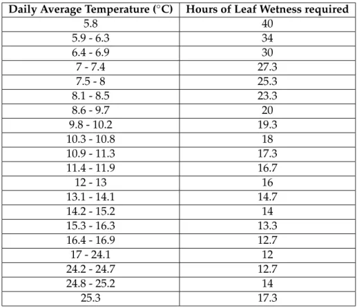
To determine disease infection risk levels, the model calculates the daily average tem-perature and measures the hours of leaf wetness required for heavy infection.

Table 2.1: Hours of wetting required for heavy infection in Model 1

Daily Average Temperature (◦_C) _{Hours of Leaf Wetness required}

5.8 40

5.9 - 6.3 34

6.4 - 6.9 30

7 - 7.4 27.3

7.5 - 8 25.3

8.1 - 8.5 23.3

8.6 - 9.7 20

9.8 - 10.2 19.3

10.3 - 10.8 18

10.9 - 11.3 17.3

11.4 - 11.9 16.7

12 - 13 16

13.1 - 14.1 14.7

14.2 - 15.2 14

15.3 - 16.3 13.3

16.4 - 16.9 12.7

17 - 24.1 12

24.2 - 24.7 12.7

24.8 - 25.2 14

25.3 17.3

For example, according to the model, at a daily average temperature of 12.5◦C, 16

hours of leaf wetness are required for heavy infection. See Table 2.1.

The temperature ranges in Table 2.1 have been adapted from the original table pro-vided in [9], whose temperatures are specified in the Fahrenheit scale.

Once infection has occurred, the model switches to the risk assessment phase and is based entirely on the effect of temperature on the reproductive rate of the pathogen.

Stage 2

(31)

It is based on a set of rules which depending on temperature variation, an index is incremented or decremented so that according to its value, one can verify when it is necessary to apply proper products.

1. Index starts at 60.

2. For each subsequent day where at least six continuous hours of temperatures be-tween 21.1 and 29.4◦C occur, index increases by 20.

3. If there are less than six consecutive hours of temperatures between 21.1 and 29.4◦C,

index decreases by 10.

4. If the temperature is 35◦C or higher for at least 15 minutes, index decreases by 10.

5. If on the same day with 6 continuous hours between 21.1-29.4◦C the temperature

exceeds 35◦C for 15 minutes or more, index increases by 10.

6. Index is never lower than 0 or higher than 100.

7. In one day the index can’t decrease by more than 10 or increase by more than 20.

Conclusions:

• Index of 30 or less indicates that a spray interval can be stretched to the label

maxi-mum of the product.

• Index of 40 to 50 indicates that a spray interval can be of intermediate length.

• Index of 60 to 100 indicates that there is high pressure for powdery mildew and

spray intervals should be shortened to the label minimum.

• After treatment, the index is reset to zero.

2.2.1.2 Model 2: PMI

This powdery mildew model is due to [13], and like the other model, a summary of the model can be found in [9] from which we adapted the following description.

Environmental input variables:

• Daily high and low temperatures

• Precipitation

First dusting should occur twelve days after initial leaf appearance or 15 cm shoot growth.

Subsequent dustings should occur when the difference between the current PMI and the PMI on the last dusting date equals or exceeds 1.0.

When precipitation exceeds 0.25 cm, the vineyard should be re-dusted.

(32)

Table 2.2: Daily indexes for high and low daily temperatures in Model 3: PMI

Low Daily high temperature —_13-16 _16-18 _18-21 _21-24◦C _24-27 _27-29 _29-32 _32-35 _35-38 _38-41 _41-43

4-7 0.083 0.083 0.083 0.083 0.083 0.077 0.067 0.067 0.056 0.05 0 0.043 7-10 0.083 0.083 0.083 0.083 0.091 0.083 0.077 0.067 0.059 0.05 3 0.048 10-13 0.083 0.083 0.083 0.083 0.100 0.091 0.083 0.077 0.063 0.05 9 0.053 13-16 0.083 0.083 0.083 0.091 0.111 0.100 0.091 0.083 0.077 0.06 3 0.059 16-18 —- 0.083 0.083 0.111 0 .111 0.111 0.100 0.091 0.077 0.071 0.067 18-21 —- —- 0.100 0.143 0. 143 0.125 0.125 0.100 0.091 0.077 0.071 21-24 —- —- —- 0.143 0.1 67 0.143 0.125 0.111 0.091 0.077 0.067 24-27 —- —- —- —- 0.14 3 0.125 0.091 0.083 0.067 0.056 * 27-29 —- —- —- —- —- 0.091 0.077 0.059 * * * 29-32 —- —- —- —- —- —- 0.059 0.059 * * * * The amount of product applied should be reduced to avoid excess leaf burn.

2.2.2 Grape downy mildew

We follow closely the explanation of downy mildew disease found in [8] and [14]. In short, downy mildew is a highly destructive disease of grapevines across all wine regions of the world where it rains in the spring and summer with temperatures above 10◦C.

Harvest losses in single years can be up to 100% if the disease is not controlled during favorable weather conditions.

Currently, there are no adequate sources of resistance in commercially acceptable va-rieties, causing fungicides to be the primary means of controlling the disease.

2.2.2.1 Model 1: 3-10 rule

This downy mildew model is due to [15], from which we adapted the following descrip-tion.

Input variables:

• Air temperature

• Current phenological state

• Rainfall of last 48 hours

This empirical model is very simple. It verifies disease occurrence if there are simul-taneous occurrence of the 3 following conditions:

1. Air temperature equal or greater than 10◦C

2. Vine shoots higher than 10 cm. (Possible to verify on the current phenological state of plant)

(33)

Figure 2.5: Grape plant affected with downy mildew [9]

2.2.2.2 Model 2: EPI

Like the other model, a summary of the model can be found in [15] from which we adapted the following description.

Input variables:

• Climatic monthly values of: rainfall, temperature, number of rainy days, nocturnal

average of relative humidity

• Montly values of: rainfall and average temperature

• Decade (10 days) values of: rainfall and number of rainy days.

• Average diurnal relative humidity between 10:00 hours and 18:00 hours

• Average daily temperature

Climatic values are average values calculated for a relatively long and uniform pe-riod, being of at least thirty consecutive years.

(34)

Stage 1: Potential energy

Potential energy is calculated between 1 October and 31 March, with a time step of 10 days, based on the differences in air temperature and rainfall of the current year com-pared to the climatic average calculated over a 30-year period, according to the following equation:

P e= "

2∗ct √Rm₋ r

Rm_∗95 100 !# + ( 0.2∗ " √

Rm_∗√T m₋ r

Rm_∗95 100 ∗ √ T m !#) −

RDm_∗1.5 18

∗log Rd RDd

Where,

• P e=potential energy

• ct= 1.2in October - November;1in December;0.8in January, February and March;

• Rm=climatic monthly rainfall;

• T m=climatic monthly temperature;

• RDm=climatic number of rainy days per month;

• T m=average monthly temperature;

• Rm=monthly rainfall;

• Rd=rainfall in the decade (10 days);

• RDd=number of rainy days in the decade (10 days).

Stage 2: Kinetic energy

Kinetic energy is calculated every day between 1 April and 31 August, according to the following equation:

Ke= 0.012_∗     

5_∗RHm+ 3RHi 8

2

∗√T i₋RHi2_∗√T m

(35)

• Ke=kinetic energy;

• RHm=climatic monthly nocturnal average of relative humidity;

• T m=climatic monthly temperature;

• RHi=average diurnal RH between 10.00 hours and 18.00 hours;

• T i=average daily temperature.

Summation of equations gives the EPI index as follows:

EP I =

M arch

X

October

P e+

September

X

April

Ke

This model considers that the first seasonal infection occurs whenEP I >−10.

2.2.3 Tomato diseases

Early blight is perhaps the most common foliar disease of tomatoes. This disease causes direct losses by the infection of fruits and indirect losses by reducing plant vigor [16].

Septoria leaf spot is one of the most common foliar diseases of tomato. It can be highly destructive given the proper conditions and has been known to cause complete crop fail-ure. Although the causal fungus will not directly infect the fruit, losses are the result of defoliation which can lead to the failure of fruit maturation and sunscald of exposed fruit [17].

Anthracnose is a tomato disease that produces black, sunken lesions on the ripening fruit. Although symptoms do not appear until the fruit is ripening, the infection actually occurs when fruits are small and green [18].

2.2.3.1 Model 1: TOMCAST

This model is due to [19] from where we adapted the following description.

TOMCAST (TOMato disease foreCASTing) is a computer model model that uses lo-cal weather conditions to predict fungal disease development, on tomatoes, specifilo-cally Early Blight, Septoria Leaf Spot and Anthracnose.

Input variables:

• Hourly average temperature per day

(36)

The TOMCAST model index is determined by two factors, leaf wetness and tem-perature during the leaf wet hours. As the number of leaf wet hours and temtem-perature increases, the index accumulates at a faster rate, i.e., increased disease pressure. Con-versely, when there are fewer leaf wet hours and the temperature is lower, the index accumulate slowly if at all, i.e., decreased disease pressure. The table below shows the interaction between those two factors:

Table 2.3: Daily indexes for TOMCAST model

Average Temperature During Leaf Wet Hours Hours of Leaf Wetness per Day 13-17 degree C 0-6 7-15 16-20 21 +

18-20 degree C 0-3 4-8 9-15 16-22 23+ 21-25 degree C 0-2 3-5 6-12 13-20 21+ 26-29 degree C 0-3 4-8 9-15 16-22 23+

Daily Index = 0 1 2 3 4

When the accumulated value of the index exceeds a pre-determined limit, the spray threshold, a fungicide spray is recommended to protect the foliage and fruit from disease development.

The spray threshold can range between 15-20. By following a 15 index spray thresh-old, a more conservative use of the TOMCAST system, a grower will apply fungicides more frequently than a grower who uses a 20 index spray threshold.

2.2.4 Models validation

Below, we discuss the validations made of the models previously described. However, it is not the purpose of this dissertation to validate these models, it is only important to know whether they can be efficiently used.

(37)

2.2.4.1 Grape powdery mildew

Both the powdery mildew models were validated in multiple growing regions of Califor-nia and the first model is actually being implemented in several grape-growing counties of the state [9].

Both Portugal and California have Mediterranean climate making their weather very similar, the difference is the fact Portugal summer heat is tempered by the Atlantic influ-ence instead of the Pacific [20].

In Mediterranean climates, wine regions have long growing seasons of moderate to warm temperature and winters are usually warmer than those of maritime and continen-tal climates. This leads to very small amounts of rain fall, requiring that farmers water grapes more often due to the increase of drought risk [21].

The first model is also currently being validated in New York, Washington, Oregon, Germany, Austria and Australia.

2.2.4.2 Grape downy mildew

The grape downy mildew models are already being used by a Portuguese institution called COHTN1 _{(Centro operativo e tecnológico hortofrutícula Português). They also} provide results of these models in their website.

2.2.4.3 Tomate lateblight

Both TOMCAST and BLITECAST were validated in the Region of Ribatejo from 2002-2005 [22], and shown appropriate with small changes. BLITECAST is a model adapted from TOMCAST for the potato late blight disease.

Currently, and according to our partnership in the PROTOMATE project, it was told to us that the TOMCAST model is currently being validated in Portugal by a major multi-national company.

2.3 Data required

In order to be able to calculate diseases infection risk with the previous models, it is required to obtain weather values for various locations.

There are two types of data being used:

• Environmental

• Calculated

In our approach, environmental values are provided by the "Instituto Português do Mar e da Atmosfera", and these values can be obtained via:

• Satellite.

(38)

• Weather stations spread throughout the country.

We also have online access to historical data from SNIHR2_{(Sistema Nacional de} In-formação de Recursos Hídricos), which is the portuguese national information system for water resources. They have meteorological information from their own weather stations of the previous 20 years. However these stations are no longer being maintained.

Additionally there might also be environmental values from farmers which have their own weather stations and want to use their values as input.

Calculated values are values that can’t be obtained via satellite or from a weather station so it is necessary to estimate them using mathematical models. Currently, it is only required to calculate one value: leaf wetness.

2.3.1 Environmental

2.3.1.1 Satellite

The satellite that collects meteorological data is the EUMETSAT3_{Satellite, and this} infor-mation is provided by the LAND SAF4_{, which is a system that provides analysis of land} surface temperature. LAND SAF is also maintained by the IPMA.

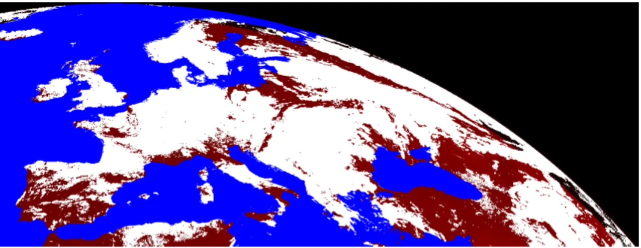
Satellite information is obtained by satellite images where for each pixel of the image its possible to obtain the latitude, longitude and the corresponding value of the land surface temperature of an area of roughly a square of 4 by 4 kilometres, at the portuguese latitudes.

Figure 2.7: Example of a LST satellite image

In the figure 2.10, the colours represent:

• Black: Unavailable data

• Blue: Water pixels

2_{http://snirh.pt/}

3_{http://www.eumetsat.int/}

(39)

• White: Pixel covered with clouds, therefore value might be not available or

inaccu-rate

• Red: Pixel with available land surface temperature value

The information is provided in files of HDF5 format, which can be easily read by software. Is is available in a FTP server hosted by our collaborators in Universidade de Évora.

Since we’re working with satellite data, sometimes due to cloud coverage it might be impossible to obtain some values for a specific region. These lacks of information will be obviated by calculating some estimative of the temperature using spatial interpolation algorithms.

The satellite provides this information every 15 minutes, occurring 96 times per day. As of this moment its possible to obtain via satellite the following data:

• Land surface temperature at periods of 15 minutes

In the future, if other satellites or other types of environmental data are available, they can be easily included in our platform (e.g. precipitation).

2.3.1.2 Weather stations

There are a total of 146 weather stations from Instituto Português do Mar e da Atmosfera located in Portugal and all of them provide hourly data with values at its current location (See Table 2.4).

This information can be less accurate than information from satellite due to lack of maintenance and there are few less number of weather stations than locations where satellite data is available.

IPMA has some meteorological information from their weather stations in their web-site, providing data from the previous 5 days for any station.

2.3.1.3 Mobile phone sensors

One of the most expected features in mobile devices in the future is the integration with environmental sensors to detect values like temperature and relative humidity at the exact place where the device is.

Since it is planned the development of a mobile application, it would allow our sys-tem to have another information provider.

Android has recently introduced the new sensor API5_{for humidity and temperature,} but after investigating and searching it was not possible to find any mobile devices on the market with those built-in sensors, and therefore implementation was not performed. It will however be considered in possible future contributions.

(40)

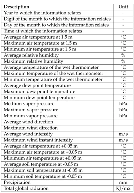
Table 2.4: Information provided by each weather station.

Description Unit

Year to which the information relates -Digit of the month to which the information relates -Day of the month to which the information relates -Time at which the information relates -Average air temperature at 1.5 m ◦C

Maximum air temperature at 1.5 m ◦C

Minimum air temperature at 1.5 m ◦C

Average relative humidity %

Maximum relative humidity %

Average temperature of the wet thermometer ◦C

Maximum temperature of the wet thermometer ◦C

Minimum temperature of the wet thermometer ◦C

Average dew point temperature ◦C

Maximum dew point temperature ◦C

Minimum dew point temperature ◦C

Medium vapor pressure hPa

Maximum vapor pressure hPa

Minimum vapor pressure hPa

Average wind direction Maximum wind direction

Average wind intensity m/s

Maximum wind instant intensity m/s Average air temperature at +0.05 m ◦C

Maximum air temperature at +0.05 m ◦C

Minimum air temperature at +0.05 m ◦C

Average soil temperature at -0.05 m ◦C

Maximum soil temperature at -0.05 m ◦C

Minimum soil temperature at -0.05 m ◦C

Precipitation mm

Total global radiation KJ/m2

2.3.2 Calculated

2.3.2.1 Leaf wetness

One of the most important input variables for the more complex mathematical models is leaf wetness.

Leaf wetness duration is the period of time during which free water – from dew, rainfall, fog, or irrigation - is present on the aerial surfaces of crop plants [23]. It is used for monitoring leaf moisture for agricultural purposes, such as fungus and disease control, for control of irrigation systems, and for detection of fog and dew conditions, and early detection of rainfall [23].

(41)

Figure 2.8: Example of leaf wetness present on a leaf. [24]

To predict the presence of leaf wetness there are many mathematical models, however in this case we’re limited to the weather data provided, so three usable models were found:

• Constant threshold

• Extended threshold

• CART/SLD/Wind model

A potential advantage of these empirical models is that they may be used to estimate leaf wetness from either on-site weather measurements, offsite or remotely estimated data, or both [25].

Constant threshold [26]

Constant threshold model is a simple model that only has one input variable: relative humidity (RH).

This method assumes that leaf is considered wet if RH is greater than or equal to a constant threshold. It was developed from observations that condensation on grass cover began before saturation in the air was reached, when relative humidity ranged from 91% to 99%.

(42)

Extended threshold [26]

Like the constant threshold model, this model only requires air relative humidity as an input.

The extended threshold approach considers hours in which RH is higher than 87% as wet hours. For values of RH between 70% and 87%, an hour is considered wet if RH is at least 3% higher than the RH of the hour before and dry if RH is at least 2% lower than the RH of the hour before. The hours in which RH is lower than 70% are considered dry. If these conditions are not satisfied, the hour is considered the same as the previous one.

CART/SLD/Wind model [25]

CART/SLD/Wind is a nonparametric empirical model for estimating leaf wetness duration using classification and regression tree (CART) analysis with stepwise linear discriminant analysis (SLD). In order to calculate leaf wetness status it is required to obtain initial input data:

• Dew point depression (air temperature - dew point temperature)

• Wind speed

• Relative humidity

All this data is available via weather stations located nearby.

This model uses a CART Tree and in 2 situations it has to verify an inequality to calculate leaf wetness.

The inequalities are:

(1.6064√Tair+0.0036Tair2 +0.1531RH−0.4599W ind×DP D−0.0035Tair×RH)>14.4674

(Inequality 1)

(0.7921√Tair+0.0046RH−2.3889W ind−0.0390Tair×W ind+1.0613W ind×DP D)>37.0

(Inequality 2)

Where,

• Tair=Air temperature◦C.

• RH =Relative humidity %.

• W ind=Wind speed m/s.

(43)

Figure 2.9: Classification tree for prediction of leaf wetness [25]

2.3.3 Spatial interpolation

Due to the fact information obtained is dependent on the location of weather stations and satellite accessible points, it becomes necessary to calculate approximate values for other locations.

Spatial interpolation is the process of using points with known values to estimate values of other points. It concerns a set of techniques designed to create continuous surfaces from sample points.

The techniques researched include deterministic methods of interpolation such as Nearest Neighbour, Inverse Distance Weighting, and the Kriging stochastic method.

Deterministic models assign values to geostatistic locations based on the surrounding measured values while stochastic methods are based on statistical models that include autocorrelation.

2.3.3.1 IDW (Inverse distance weighting) [27]

The inverse distance weighting method is a deterministic interpolation procedure (as opposed to a stochastic process) that uses a separate data set, typically in space.

The locations of unknown value are calculated using a weighted average of the in-verse of the distance from that location to the location of known values.

(44)

2.3.3.2 Nearest neighbour [28]

Nearest neighbour interpolation is a deterministic method of interpolation where the estimated value is always equal to its nearest sample.

Due to its simplicity is regularly used for quick interpolations, and in areas well sam-pled.

2.3.3.3 Kriging [27]

Kriging is a stochastic regression method used in geostatistics to interpolate data.

It is similar to IDW in that it assumes that nearby points in space tend to have more similar values than points farther apart.

To do so it uses a linear combination of weights at known points to estimate values at unknown points. These weights change according to the spatial arrangement of the samples.

2.4 PROTOMATE project and data problems

"PROTOMATE - uma ferramenta de apoio à gestão da cultura do tomate para indús-tria" (PROTOMATE - a tool to support the management of tomato crop for industry) is a project that aims the development of a software tool to deal with a tomato pest called

Tuta absoluta. It has the contributions of several different organizations:

• "COTHN - Centro Operativo e Tecnológico Hortofrutícola Nacional", a portuguese

center for technological operations of fruits and vegetables.

• "ESAS - Escola Superior Agrária de Santarém"

• "ISA - Instituto Superior de Agronomia"

• "UE – Universidade de Évora"

• "FNOP- Federação Nacional de Organizações de Produtores", the national

federa-tion of farmer groups.

• LUSOSEM, an agriculture products company.

• And AGROMAIS,15 other farmer organizations.

Due to the similarities between my dissertation and the project, I had a research schol-arship for the University of Évora, under guidance of Prof. José Rafael Silva to develop some functionalities on the platform so they could make data analysis with the data ob-tained via satellite and from weather stations.

(45)

2.4.1 Current issues

2.4.1.1 Temperature

Air temperature and land surface temperature are significantly different. Air tempera-ture is usually the temperatempera-ture measured at 1.5 meters of the ground, and land surface temperature is the temperature measured exactly at ground level.

These 1,5 meters can make a big difference when using temperature values in our em-pirical models since all models require air temperature and not land surface temperature. Air temperature can be obtained via weather stations and land surface via satel-lite. However weather stations have weak maintenance and its values can’t be entirely trusted.

For this, it is necessary to make an application in order to help create a correlation between these two values.

2.4.1.2 Humidity

Relative humidity is essential for disease models since it is one of the most important input variables and is required to obtain leaf wetness values.

At this moment there are several studies made which provide a way of obtaining relative humidity from dew point temperature and air temperature. However, like in the previous section, all these data types are only available from weather stations and so, a solution is required.

Based on current investigations, Prof. José Rafael Silva is researching a way of de-termining relative humidity based only on temperature. He conjectures that creating a relative humidity index can be important in estimating relative humidity values from the land surface temperature.

The formula is as follows:

RHIndex= M axV alue−M inV alue ∆t

Where M axV alueis the maximum value of land surface temperature verified in a day, andM inV alue is the minimum value respectively. Also, ∆t is the time between occurrence ofM axV alueand the occurrence ofM inV aluein hours.

2.4.2 Time-series segmentation

Time-series segmentation is the proposed solution by Prof. José Rafael Silva to try to solve our data problems and allow further analysis on the data.

It is a method of time series analysis, in which time the input series are divided into a sequence of segments, and produce a piecewise linear representation.

There are 3 possible segmentation algorithms[29]:

• Sliding Windows: A segment is grown until it exceeds some error bound. The

(46)

Figure 2.10: Two examples of time series segmentation. The figures above display the time series, and below its segmentation.[29]

• Top-Down: The time series is recursively partitioned until some stopping criteria is

met.

• Bottom-Up: Starting from the finest possible approximation, segments are merged

until some stopping criteria is met.

2.4.2.1 Solar calculations

Since we are working with time series and using temperature values, some other impor-tant information could be useful while analyzing our data.

For that we chose to calculate the time at which sunrise, sunset and solar noon occur at a specific day in a specific location.

We calculate these times using solar calculation formulas provided by NOAA/ESRL’s Global Monitoring Division6_{. These formulas are found in [30].}

Fractional year in radians:

y= 2π

365∗(day_of_year−1 +

hour₋12

24 )

Equation of time in minutes:

eqtime= 229.18_∗(0.000075+0.001868 cosy₋0.032077 siny₋0.014615 cos 2y₋0.040849 sin 2y)

Solar declination angle in radians:

decl= 0.006918₋0.399912 cosy+ 0.070257 siny₋0.006758 cos 2y+ 0.000907 sin 2y₋ 0.002697 cos 3y+ 0.00148 sin 3y

For sunrise and sunset, the zenith is set to 90.833 degrees (the approximate correction for atmospheric refraction at sunrise and sunset).

(47)

The hour angle in degrees:

ha= arccos ( cos (90.833)

cos (lat) cos (decl) −tan (lat) tan (decl))

Then, UTC for sunrise in minutes is:

sunrise= 720 + 4(longitude₋ha)₋eqtime

And sunset:

sunset= 720 + 4(longitude+ha)₋eqtime

Also, it is possible to obtain the solar-noon in minutes:

solar_noon= 720 + 4∗longitude₋eqtime

2.5 Conclusions

In conclusion, this chapter viewed the main subjects to be addressed.

In the models of disease prevention, it is observed that the most important input values are temperature and duration of hours when leaf wetness occurred. To calculate leaf wetness, the main input value is relative humidity, being also possible to increase the accuracy of the results if wind speed and dew point temperature are known.

This data can be obtained from satellite and weather stations. However, at present, it is only possible to obtain the value of surface temperature from the satellite, being required to also obtain values from weather stations for the most complex models.

(48)

(49)

3

Approach

This chapter describes every step of the development of the constructed system. It fo-cuses in explaining what was implemented and what were the priorities.

3.1 Solution presented

Our solution consists of a system that obtains meteorological data, calculates the possi-bility of infection in cultures and at the same time allows interaction to users via mobile devices, recording treatments and possible culture enemies observed.

For this, it was developed:

1. A database to store all information.

2. Algorithms to obtain data from satellite and weather stations and store them in the database.

3. Implementation of leaf wetness and disease models, storing results in database.

4. Scripts that allow analysis of the temporal data in the system.

5. Web-services to provide results and ability to make queries to the database.

6. Mobile application for users to interact with the system.

(50)

applications. An example of such applications are the data analysis functions that were developed.

In the Figure 3.1 the arrows represent the direction in which information flows. For example, satellite data is only sent to the system, while in mobile applications informa-tion can be received from the system (notificainforma-tions) and can be sent from the mobile (user interactions).

Satellite Data Weather Station Data

Spatial Database

Mobile Application Web Services

Analysis Functions Disease Models

(51)

3.2 Database

A database was necessary to store all the data gathered by the system. This includes weather data, results from disease models, and observations made by the user.

Besides temporal data, our database will also store information regarding the agricul-tural domain. It includes all necessary information by the field notebooks, such as plants, plant enemies, users and their plots, traps, products, etc.

3.2.1 Database type

Since we are working with geographical information it was required to use a spatial database. A spatial database is a database that is optimized to store and query data that is related to objects in space, including points, lines and polygons.

While typical databases can understand various numeric and character types of data, additional functionality needs to be added for databases to process spatial data types. These are typically called geometry.

3.3 Web server

After having a database, it was required to develop an information platform that would interact with it, collecting weather information, calculating status of possible diseases and providing this information to the user.

For that, a server was built, which is always running and ready for incoming calls from mobile applications. Its main requirements are:

• Weather data acquisition - It should be able to obtain data from sources and store it

in the database.

• Run plant enemy models - Should run daily models with information previously

obtained.

• Web services - In order to connect with mobile application

• Other important applications - Extra scripts with access to the database

3.3.1 Weather data acquisition

Four scripts were created to download and insert meteorological data:

• A script to download recent HDF5 files from the FTP server and store the satellite

data in the database.

• A script to download weather station data from previous 5 days in www.ipma.pt

and insert it in database if not inserted already.

(52)

• A script to read from local Excel files containing weather station data and store it.

Whenever possible, it is required for the web server to run these scripts since there is new data every 15min for satellite and 1h for weather stations. However these could usually be done daily before executing plant enemy models since that is the only time the data is truly necessary.

Due to cloud coverage, sometimes the satellite can’t provide the temperature of cer-tain locations. To overcome this problem we use interpolation algorithms to predict these values in order to maintain accuracy of mathematical models.

The interpolation algorithm chosen to be implemented is the Inverse Distance Weight since it is algorithm used by the IPMA (Instituto Português do Mar e da Atmosfera).

3.3.2 Run plant enemy models

Usually on a daily basis our server executes the enemy models in order to calculate the risk of plant infection in all user plots.

To do so the models for disease prediction were implemented for all diseases ad-dressed.

A generic architecture was created to allow plugging in easily other models for other diseases and pests in future contributions. This way the system provides scalability for every new model that is available to be inserted.

3.3.2.1 Calculating leaf wetness

While executing each model, if leaf wetness is necessary and not available, then it will be calculated.

The three models were chosen to be implemented. Depending on the available data, the system tries to use CART/SLD/Wind since it is the most accurate of the three.

All these calculated values are also stored in the database to help in future usages and/or statistical analysis.

3.3.3 Web services

In our server, we provide a web service for mobile applications to interact, allowing them to obtain information about a specific location and to manually enter data, such as specific stage of a plant according to the opinion of the technician and updated images of a plant with a possible disease.

The basic web methods available are:

• User login

Users are able to log in the system and have an account associated.

• Get user farms and plots information

(53)

• Get model results

Present model results from the current day for a specific plot.

• Receive information about user interactions such as:

– Treatments made

– Culture enemy observed

– Insect traps observation

These reflect the actions required in the field notebooks. They are always stored in the database.

When submitting an interaction, the user must always supply the specific plot, the plant being analyzed, its enemy and the current phenological stage of the plant.

The user might also add some additional text to enhance the observation made.

3.3.4 Analysis functions

Since the system will have access to the database there are inumerous possible functions that can be made.

Also, as previously stated, our collaborators in the PROTOMATE project asked us to implement some analysis functions using our database, so they could make posterior analysis on the results.

3.3.4.1 Time-series segmentation

In order to solve these 2 problems, two scripts were created that based on data in our database, create an image with a linear representation of time series segments for two different data types from satellite and weather stations. One script is for the comparison between land surface temperature from satellite and air temperature at 1.5 meters from weather stations, and the other between land surface temperature from satellite and air temperature at 0.05 meters from weather station.

In the image, besides the segments, we also present some additional information of each particular day. First we display the time at which sunrise, sunset and solar noon occurred, displaying also vertical bars in our time series at each of these times.

Then, we present the maximum, minimum and average value of each time series. In addition, we also show the relative humidity index calculated and the time between the occurrence of the maximum value and the occurrence of the minimum value in hours.

The scripts also create 2 files each with values from the segments presented. These files are in the CSV format.

(54)

Figure 3.2: Example of the linear representation of time series with Sliding Windows algorithm.

(55)

Preliminary findings show a strong correlation between land surface temperature and the air temperature at 0.05 meters, obtained via weather stations. These were possible to obtain due to our system.

3.4 Mobile application

Our primarily user interface is trough a mobile application for Android.

The development of a mobile application was important for farmers and agronomists to use in order for them to request the results from our disease models and allow them to manually submit interactions such as plant treatments, disease observations and plant phenological stages.

However, due to lack of time, the application created is only a prototype and requires future modifications in order to be fully functional. We focused on allowing the user to see their farms and plots, and for each plot check the model results and submit some interactions he wishes to make.

The requirements were:

• Native application for a mobile device.

• Show user information regarding its farms and plots.

– He should be able to see its farms, plots, plants, traps and interactions made.

• Show user the models results for its plots.

• Allow the user to submit user interactions to the server. These interactions could

be:

– Add disease observation

– Add product treatment made

– Add trap observation

– Add an observation of a plant current phenological stage

(56)

(57)

4

State of the Art

In this section are presented technologies, tools and applications that were considered to be used in the development of the proposed solution.

First, possible database management systems are reviewed, focusing on the impor-tant features for the implementation of this work, in particular their ability to store and process geographic information.

Then, various options for the implementation of our information systems are dis-cussed, briefly detailing their interaction capabilities with our data.

Finally, a summary is made on possible technologies for the implementation of our mobile application.

4.1 Database

There are several database management systems that support geographical data. How-ever for this project is necessary to focus on open source software, noticeably:

• PostgreSQL

• MySQL

• SQLite

(58)

4.1.1 Possible options

4.1.1.1 PostgreSQL

PostgreSQL1 _{is an Open Source database management system able of handling large} sized databases.

Today PostgreSQL DMBS is one of the most advanced Open Source DBMS, with fea-tures such as: complex queries, foreign keys, transactional integrity, multi-version con-currency control and an extension to store geographical data called PostGIS.

PostGIS

PostGIS2 _{is an open source software library that allows PostgreSQL to be used as} a backend spatial database for geographic information systems, by adding support for geographic objects in its object-relational database.

Some of its main features are the addition of geometry types for points, multi-points, line strings, multi-line strings, polygons and multi-polygons.

PostGIS supports both geometry (x, y) and geography (lat, long) types and functions. It also has very usefull functions for calculating distances between locations using different coordinate systems.

4.1.1.2 MySQL

MySQL3_{is a database management system (DBMS), which uses the SQL language} (Struc-tured Query Language) as an interface.

It is currently one of the most popular database systems, with over 10 million instal-lations worldwide.

Some of the great advantages of using MySQL are its portability, compatibility, excel-lent performance and stability, little demand for hardware capabilities and ease of use.

MySQL supports a multitude of geometry types, but only on a 2D plane. The geogra-phy type systems (lat, long) are not implemented, making it an option not viable for our system.

4.1.1.3 SQLite

SQLite4_{is a C language library that implements an SQL database embedded. Programs} that use the SQLite library can have access to SQL database without running a separate RDBMS process.

SQLite is not a client library used to connect to a big database server, but the server itself. The SQLite library reads and writes directly to and from the database file on disk.

1_{http://www.postgresql.org/}

2_{http://postgis.net/}

3_{http://www.mysql.com/}

(59)

Spatialite

Spatialite5_{is a variant of the SQLite database that provides GIS features. It uses the} GEOS, PROJ.4, etc... libraries that are also used in PostGIS, and hence the resulting fea-ture set is similar.

Only geometry types (2D x,y operations) are supported, making the lack of support for geography projections (lat, long) one major issue like MySQL.

However, since mobile operating system Android uses SQLite databases on the de-vice, Spatialite might be useful for implementation of other functions.

4.1.2 Database chosen

The database system chosen is PostgreSQL with PostGIS.

PostGIS allow us to associate satellite information to specific points and relate the areas of plots to polygons, or single points, making it possible to take advantage of these point coordinates for possible data interpolations required to obtain missing values or required values in specific locations.

4.2 Web server

In the server-side there are inumerous options. In order to ease this decision, it was opted to develop using Java programming language and its SDK technologies since it is the language the candidate had most experienced with and it has plugins/libraries for implementation of all the requirements.

4.2.1 Apache Tomcat

Apache Tomcat is an open source web server and servlet container developed by the Apache Software Foundation (ASF).

It will be used to start the system being always available for any incoming connection.

4.2.2 JAX-RS and Jersey

The web-services in our server were made in a RESTful API, using JAX-RS for it’s devel-opment along with Jersey.

JAX-RS: Java API for RESTful Web Services is a Java programming language API that provides support in creating web services according to the Representational State Transfer (REST) architectural pattern.

Jersey is a reference implementation of JAX-RS, which implements support for the an-notations defined in JSR 311, making it easy for developers to build RESTful web services by using the Java programming language.

(60)

4.2.2.1 Jackson

Also a library called Jackson was used to allow parsing of JSON objects received from the mobile application and being sent to it.

Jackson is a multi-purpose Java library for processing JSON data format. With the extension Jackson-JAXRS-JSON it is possible to handle JSON input/output for JAX-RS implementations (like Jersey and RESTeasy) using standard Jackson data binding.

4.2.3 PostgreSQL JDBC

PostgreSQL JDBC allows Java programs to connect to a PostgreSQL database using stan-dard, database independent Java code.

It provides a reasonably complete implementation of the JDBC 3 specification in ad-dition to some PostgreSQL specific extensions.

4.2.4 HDF Object Package

The HDF Object Package is a Java package that provides an object-oriented interface to HDF data objects. The package offers a common API to access both HDF4 and HDF5 files.

It allows the development of easy routines to read the HDF5 files with temperature values from the satellite and store them in the database.

4.3 Mobile application

Our primarily user interface will be trough a mobile application.

4.3.1 Operating system

There are 3 main operating systems to develop mobile applications:

• Android

• iOS

• Windows Phone 8

4.3.1.1 Android

Android6 _{is an operating system based on Linux for mobile devices. It is developed by} the Open Handset Alliance led by Google and other companies.

According to Google, more than 1 million 300 thousand devices with this operating system are activated every day.

(61)

4.3.1.2 iOS

iOS7 _{(formerly iPhone OS) is a mobile operating system from Apple Inc. originally} de-veloped for the iPhone.

Interaction with the OS includes gestures such as just tapping the screen, slide your finger, and the movement of "tweezers" used to enlarge or reduce the image.

4.3.1.3 Windows Phone 8

Windows Phone 88_{is the second generation of Windows Phone mobile operating system} from Microsoft.

Nokia announced a partnership with Microsoft in February 11, 2011 becoming its main operating system.

4.3.1.4 Operating system chosen

As far as operative systems, Android was chosen due to being the most popular oper-ative system for mobile devices and for being the simplest operoper-ative system to develop applications.

Android phones are cheaper than iPhones and a previous poll to an “Associação de Produtores” led us to conclude that there is a preference for recent Android phones.

Windows Phone 8 is still new in the market so it will be dropped as third and last option.

In addition, the candidate also had experience in developing applications for An-droid, making it the most viable option.

4.4 Conclusions

In conclusion, several technologies were chosen to be used for the implementation of our project.

For the database, we opted for PostgreSQL with PostGIS. In the server we chose Apache Tomcat server and the creating of a RESTfull API with Jersey. Lastly, the mo-bile application is made for the Android operating system.

7_{http://www.apple.com/ios/}

(62)

(63)

5

Database

In this chapter a detailed explanation of the database implementation is described. First, the database diagrams are showed and briefly explained, then we focus on spe-cific code for database creation and interaction.

5.1 Database model

The database can be divided in 2 sections for better understanding:

• Geographical and temporal data

• User interactions

5.1.1 Geographical and temporal data

In this section, it is presented how the database was structured to store temporal data from any kind of sources. The following is a summary of each table and its relationships:

5.1.1.1 Organizations

These are simple organizations that provide the data to be stored in the database. For example, in our case the organization that provides both satellite data and meteorological data is IPMA.

5.1.1.2 Source Types

Field Information Web Platform for Agricultural Applications