The Economic Consequences of the Agricultural Expansion in Matopiba

(1)

The Economic Consequences of the

Agricultural Expansion in Matopiba

*

Arthur Bragança†

Contents: 1. Introduction; 2. Background; 3. Data and empirical design; 4. The characteristics of the agricultural expansion; 5. The Consequences of the Agricultural Expansion;

6. Conclusion; Appendix.

Keywords: Agriculture, Development, Agricultural Frontier. JEL Code: O13, Q13.

This paper examines the consequences of the agricultural expansion in theMatopiba— areas from the states of Maranhão, Tocantins, Piauí and Bahia located in the Cerrado biome. Comparing municipalities from these four states located inside and outside the Cerrado biome, it ﬁnds that agricultural production evolved similarly in these groups of municipalities until the late 1990s when it started to increase faster in municipalities inside the Cerrado. The growth in agricultural production led to increases in GDP per capita and access to durable goods and basic infrastructure.

Esse artigo examina as consequências da expansão agrícola noMatopiba— areas dos es-tados do Maranhão, Tocatins, Piauí e Bahia localizadas no bioma Cerrado — através da comparação da evolução de resultados econômicos de municípios desses estados localiza-dos dentro e fora do bioma Cerrado. Os resultalocaliza-dos indicam que a evolução da produção agrícola nesses grupos de municípios foi parecida até o ﬁnal dos anos 1990, quando co-meçou a crescer mais rápido nos municípios localizados no bioma Cerrado. O crescimento da produção agrícola se traduziu em crescimento do PIB per capita e do acesso a bens de consumo duráveis e infraestrutura básica.

1. Introduction

TheMatopiba—areas in the states of Maranhão, Tocantins, Piauí and Bahia located in the

Cer-rado biome—became an important agricultural frontier during the past 20 years. Agricultural expansion in this region is being driven by the expansion of soy cultivation in large-scale and mechanized farms. The production of this crop increased almost six times in the Matopiba during the period 1995–2012, doubling its share in the Brazilian soy production, and inducing multinational traders and seed producers to open units in the region. However, despite the magnitude of this agricultural expansion, there is no evidence of its consequences on economic development.

*I thank Laisa Rachter for excellent comments and suggestions and the Child Investment Fund Foundation (CIFF) for generous ﬁnancial support. All errors are my own.

(2)

To ﬁll this gap, this paper examines the consequences of the agricultural expansion in the Matopiba. To deal with the concern that agricultural expansion is endogenous, it compares the evolution of economic outcomes in municipalities from the states of Maranhão, Tocantins, Piauí and Bahia located inside and outside the Cerrado biome. This differences-in-differences design identiﬁes the effects of the agricultural expansion in the Matopiba under the hypothesis that economic outcomes would have evolved similarly across these municipalities in the absence of the agricultural expansion.

The analysis begins by using data on agricultural outcomes to characterize the agricul-tural expansion. Crop cultivation and output evolved similarly across Cerrado andnon-Cerrado municipalities until the late 1990s. Then, these outcomes started to increase faster in the Cerrado municipalities. The estimates indicates that cropland increased 3.6 percentage points more in the Cerrado municipalities while the value of agricultural production increased 140% more than in the non-Cerrado municipalities during the period 1999–2012.

The increase in the value of agricultural production was not only a result of cropland expansion. The evidence suggests that the crop mix changed in the period due to increases in the relative importance of soy cultivation and declines in the relative importance of rice cultivation. There are no signiﬁcant changes in the relative importance of other products such as maize and cassava. The estimates also indicate that the expansion in cropland induced a decrease in cattle ranching in the Cerrado municipalities compared to the non-Cerrado ones. This reallocation highlight the impacts of the agricultural expansion on rural organization in the region.

The analysis then uses data on economic performance to investigate the consequences of these changes in agriculture on the economic performance of municipalities in the Matopiba. The results provide evidence that agricultural expansion positively affected the economic per-formance of the municipalities located in the Cerrado biome. The estimates suggest that GDP per capita grew 11% more in the Cerrado municipalities than in the non-Cerrado ones in the period 1999–2012. This increase is a result of a relative growth of 37% in agricultural GDP per capita and 10% in services GDP per capita. There was no effect of the agricultural expansion on the manufacturing GDP.

The increase in the services GDP highlights the existence of an important spillover of the agricultural expansion to other industries. This spillover effect is due to an expansion in local demand connected to forward and backward linkages of agricultural activities. The existence of this spillover contrasts with the evidence fromHornbeck & Keskin(2012) who ﬁnd no effect of agricultural expansion on other sectors in the Ogalalla aquifer in the U.S. The lack of effects on manufacturing contrasts withFoster & Rosenzweig (2004) who found, during the Green Revolution in India, that agricultural expansion hindered manufacturing expansion. It also contrasts with the evidence inBustos, Caprettini, & Ponticelli(2016) andMarden(2014), who estimate positive effects of agricultural growth on manufacturing growth in Brazil and China, respectively.

(3)

whether access to consumer goods and basic infrastructure changed across Cerrado and non-Cerrado areas. The results show that the share of households with television, refrigerator, and electric power grew faster in the Cerrado municipalities than in the non-Cerrado ones in the period 2000–2010. However, no effect was found on the share of households with a car and on the share of households with access to water and sewage.

The census data is also used to investigate other adjustments to the agricultural expan-sion. No effect was found on local population and on educational outcomes. The former result indicates that migration is not a relevant issue in the region and contrasts with the experience of the occupation of other parts of the Cerrado documented byBragança (2014). The latter result indicates that the agricultural expansion neither crowds-in educational investments as in

Foster & Rosenzweig(1996) nor crowds-out these investments as inSoares, Kruger, & Berthelon

(2012).

These results provide novel evidence of the economic consequences of agricultural ex-pansion in the Matopiba region. Previous studies asMiranda, Magalhães, & de Carvalho(2014) have focused in describing the agricultural expansion in the region and have not examined its consequences. The paper provides evidence that expansion of mechanized and large-scale agriculture leads to improvements in economic performance through direct and indirect effects. This contributes to a growing literature that discusses the transformations that affected the large agricultural frontier located north of Brasília since the 1960s.1

The remainder of this paper is organized in ﬁve sections. Section 2 presents a brief description of the Matopiba region. Section 3 presents the datasets used in the empirical analysis. Section4 documents the expansion of agriculture in the Cerrado areas in the Ma-topiba region. Section5documents the impact of agricultural expansion on several economic outcomes. Section6presents some brief conclusions of the paper.

2. Background

EMBRAPA deﬁnes the Matopiba as the region located in the states of Maranhão, Tocantins, Piauí and Bahia which is covered by the Cerrado biome (Miranda et al.,2014). The expansion of soy cultivation in this region over the past two decades transformed the Matopiba into one of the most important agricultural frontiers in Brazil. In 2012, there were about than 2.5 millions hectares cultivated with soy in the Matopiba, producing more than 7 million tons of this crop and generating revenues exceeding R$5.5 billion. In 1995, as a comparison, there were less than 600,000 hectares cultivated with soy, producing about 1.3 million tons of this crop and generating revenues of R$600 million.

The growth of soy cultivation in the Matopiba observed since the late 1990s follows the growth of its cultivation in other areas of the Cerrado biome observed since the 1970s. This expansion was largely a result of technological innovations that enabled soy cultivation in

1_See_{Alston, Libecap, & Schneider} ₍₁₉₉₆_), _Jepson₍_2006a_), _Jepson₍_2006b_{) and}_{Alston, Harris, & Mueller}₍₂₀₁₂₎

for descriptions of the evolution of agricultural organization in this agricultural frontier. See alsoPfaff(1999),

(4)

tropical areas with acid and poor soils which occurred during the 1970s (Assunção & Bragança,

2015). These innovations were connected to the development of soy varieties as well as the development of better soil management techniques (Klink & Moreira, 2002). Because crop cultivation in this biome requires substantial investments in fertilizers and equipment, the expansion of crop cultivation occurs in large-scale and mechanized farms (Rezende,2002).

The timing of the expansion of soy cultivation in the Matopiba seems to be connected to the large expansion in soy cultivation observed in Brazil following the devaluation of the Brazilian Real in the late 1990s (Richards, Myers, Swinton, & Walker,2012). This expansion is thought to have reshaped economic life in the region (Lopes,2014). It is believed that neigh-boring urban areas have beneﬁted from the expansion of manufacturing and services activities with linkages to soy cultivation (Miranda et al.,2014). Furthermore, soy cultivation might also affect local economies through other channels such as migration or investments in human capital (Bragança,2014). However, because soy is cultivated in large and heavily mechanized farms, there are concerns that the gains brought might not beneﬁt the communities as a whole.

3. Data and empirical design

3.1. Data

The empirical exercises from this paper use socioeconomic data from different sources. The

Pesquisa Agrícola Municipal—a municipal assessment of agriculture in the Brazilian

municip-alities—provides annual information on cultivation, production and production value for the main crops cultivated in the country. We use data on land allocation and the value of crop production for the period 1995–2012 to map the evolution on agricultural outcomes in the Matopiba region.

The Produto Interno Bruto Municipal—a dataset with estimates of municipal economic

performance—provides annual information on GDP from the period 1999–2012. The analysis uses measures of aggregate GDP as well as GDP in the three main industries to investigate the consequences of agricultural expansion on economic performance in the region. TheCenso

Demográﬁco—the Brazilian Population Census—is also used to assess the consequences of

the agricultural expansion on local development. The analysis uses the census waves of 1991, 2000 and 2010 to examine the effects of agricultural expansion on consumption, infrastructure, migration, and schooling.

The empirical design tests whether these socioeconomic outcomes changed differentially in municipalities located in the Cerrado biome during the past decades. To implement this design, a biome map and a municipalities’ map are combined to construct a dummy variable indicating whether more than 50% of the municipal area is in the Cerrado biome. This is the main independent variable used throughout the empirical analysis.

(5)

Terrestrial Air and Temperature Database Version 3.0. In addition, information on municipal latitude and longitude is collected from the IPEADATA website.

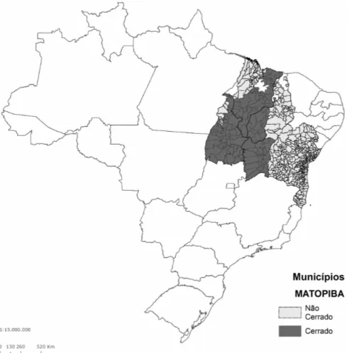
To account for border changes and the creation of municipalities, the paper uses the deﬁnition of minimum comparable areas from the Brazilian Institute of Applied Economic Research (IPEA). The minimum comparable areas make spatial units consistent over time. The estimates use a minimum comparable areas deﬁnition that makes spatial units consistent with the existing municipalities and borders from 1991. The sample is restricted to municipalities with less than 200,000 inhabitants in the initial period and with information on GDP. That leaves 665 spatial units that can be compared across periods. Throughout the paper, these minimum comparable areas are referred as municipalities. Figure 1provides a visual illustra-tion of the sample municipalities, emphasizing the ones inside and outside the Cerrado biome. There are 177 municipalities in the Cerrado and 488 municipalities outside the Cerrado.

3.2. Descriptive statistics

Table 1reports descriptive statistics for the main variables used in this paper. Column (1) presents the sample mean in the initial sample period while column (2) presents the sample mean in the last sample period. Column (3) presents the increase between periods.

Table 1.DESCRIPTIVESTATISTICS.

Observations are computed using data from all 665 municipalities in the Matopiba region.

Initial Final Difference

(1) (2) (3)

Cropland (% of municipality area) 0.039 0.048 0.009 (0.003) (0.006) (0.005) Crop Output per hectare 0.038 0.104 0.066

(0.003) (0.006) (0.005)

Soy (% of cropland) 0.078 0.194 0.116

(0.018) (0.023) (0.017) Number of Cattle (per hectare) 0.146 0.185 0.039

(0.008) (0.011) (0.006)

GDP per capita 4.779 7.774 2.995

(0.578) (0.430) (0.316)

Population 42.077 54.30 12.22

(3.002) (4.128) (1.627)

Share with TV 0.308 0.854 0.545

(0.011) (0.004) (0.008) Share with Refrigerator 0.276 0.783 0.507

(0.011) (0.005) (0.007) Share with Electricity 0.551 0.937 0.387

(0.013) (0.003) (0.011) School Enrollment (15–17) 0.485 0.831 0.346

(0.007) (0.002) (0.007) Share with 8+Years of Schooling 0.128 0.364 0.236

(6)

Figure 1.SAMPLEMUNICIPALITIES.

The figure identifies Cerrado and non-Cerrado municipalities in the states of Maranhão, Tocantins, Piauí and Bahia. Municipalities are defined as minimum comparable areas consistent with the existing municipalities and borders from 1991. Municipalities with more than 200,000 inhabitants are excluded from the sample.

The table indicates that there were substantial changes in agricultural and economic development throughout the period 1995–2012. Cropland grew about one-ﬁfth in the period whereas crop output more than tripled. Cropland expansion did not induce a reduction in cattle grazing and was connected to large shifts in land use.

(7)

Figure 2provides an illustration of the different changes in agricultural outcomes within and outside the biome. It depicts the evolution of land use and agricultural outcomes in Cerrado and non-Cerrado municipalities. The ﬁgure provides evidence that the share of cropland and the log of agricultural output per hectare grew faster inside this biome than outside of it. This evidence indicates that agricultural expansion over the past decades was indeed concentrated in the Cerrado biome as indicated byMiranda et al.(2014).

Figure 2.EVOLUTION OFAGRICULTURALOUTCOMES.

Panel A plots the evolution of the share of cropland (as % of the municipal area) in Cerrado and non-Cerrado municipalities in the period 1995–2012. Panel B plots the evolution of the log of crop output per capita in Cerrado and non-Cerrado municipalities in the period 1995–2012.

.02

.03

.04

.05

.06

.07

Cropland (% of mun. area)

1995 2012

Cerrado Non-Cerrado

Panel A: Cropland

-4.5

-4

-3.5

-3

log(Crop Output per Hectare)

1995 2012

Cerrado Non-Cerrado

Panel B: Crop Output

3.3. Empirical design

Agricultural expansion is probably inﬂuenced by characteristics like access to markets, human capital or land tenure that might directly inﬂuence economic outcomes. Therefore, OLS esti-mates of the effects of the agricultural expansion will typically be biased. To deal with this concern, the paper compares the evolution of economic outcomes in municipalities from the states of Maranhão, Tocantins, Piauí and Bahia located inside and outside the Cerrado biome. The former group is composed by the municipalities in the Matopiba which were exposed to the agricultural expansion, while the latter group is composed by municipalities neighboring the Matopiba which were not exposed to this expansion.

This empirical design identiﬁes the effects of the agricultural expansion in the Matopiba under the hypothesis that economic outcomes would have evolved similarly in Cerrado and non-Cerrado municipalities in the absence of the agricultural expansion. While it is impossible to test this hypothesis directly, it is possible to test whether outcomes were evolving similarly before the agricultural expansion began in the late 1990s.

Three different specifications are used throughout the paper. The first specification uses data on agricultural outcomes from thePesquisa Agrícola Municipalfrom 1995–2012 to charac-terize the agricultural expansion using the following model:

𝑦𝑚𝑡 = 𝛽𝑡𝐶𝑚+ 𝜃𝑡′𝐗𝑚+ 𝛼𝑚+ 𝛿st+ 𝜀𝑚𝑡, (1)

(8)

charac-teristics of municipality𝑚; and𝛼𝑚 and𝛿stare municipality and state-period ﬁxed effects. The geographic characteristics included are cubic functions of land gradient, latitude, longitude, rainfall, and temperature.

The coefﬁcients of interest in equation (1) are the different 𝛽𝑡. These coefﬁcients

rep-resent the differential change in agricultural outcomes across municipalities located within and outside the Cerrado biome that belong to the same state and share similar geographic characteristics. The different𝛽𝑡are expected to be zero before the agricultural expansion began

and different from zero after.

The main outcomes used in estimating the model in equation (1) are total cropland (as a share of the municipal area) and the log of the value of crop production (per municipal hectare). The empirical analysis also uses the share of cropland cultivated with different agricultural products to determine whether agricultural expansion was connected to changes in the crop mix.

Coefficients are pooled in two-year periods to improve precision and facilitate the vi-sualization of the results. All estimates are weighted using the total municipal area. This ensures estimates reflect the average effect for a hectare of municipal area. This weighting procedure is standard in the literature on agriculture (e.g.,Hornbeck,2012). Standard errors are clustered at the municipality-level to provide confidence intervals robust to the existence of serial correlation (Bertrand, Duflo, & Mullainathan,2004).

The second specification uses data from theProduto Interno Bruto Municipalfrom 1999– 2012 to estimate the effects of the agricultural expansion on local GDP. This empirical specifi-cation is also based on equation (1) but uses a different time period and weights the estimates using initial population to ensure the estimates reflect the average effect for a person. This weighting procedure is again standard in the literature on agriculture (e.g.,Hornbeck,2012).

The third speciﬁcation uses data from theCenso Demográﬁcofrom 1991, 2000 and 2010 to estimate the effects of the agricultural expansion on consumption, human capital, migration, and infrastructure using the following model:

𝑦𝑚𝑡 = 𝛽2000𝐶𝑚+ 𝛽2010𝐶𝑚+ 𝜃𝑡′𝐗𝑚+ 𝛼𝑚+ 𝛿st+ 𝜀𝑚𝑡. (2)

Equation (2) is similar to equation (1) which is used in the previous analysis. The main difference is that there are only two coefficients of interest (_𝛽₂₀₀₀and_𝛽₂₀₁₀). The coefficient_𝛽₂₀₀₀ indirectly tests the identification assumption that outcomes would have changed in a similar fashion in the absence of differential agricultural development in the Cerrado municipalities. The coefficient _𝛽₂₀₁₀, on its turn, investigates whether differential agricultural expansion gen-erated growth in consumption, human capital, migration, and infrastructure in the municipali-ties located in the Cerrado biome. The estimation uses the same covariates𝐗𝑚 included in the

previous estimates, weights observations using the initial population to ensure the estimates reﬂect average effects for a person and cluster standard errors at the municipal-level to deal with serial correlation.

(9)

estimates using agricultural outcomes can be interpreted as “ﬁrst-stage” estimates, while the estimates using economic outcomes can be interpreted as “reduced-form” estimates of the effects of the agricultural expansion. It is possible to combine these estimates to obtain struc-tural (Wald or instrumental variables) estimates of the economic effects of the agriculstruc-tural expansion. Nevertheless, these estimators will be a convex combination of average causal effects on different sub-populations, making their interpretation difﬁcult. Hence, the these estimators are mentioned only to contextualize the magnitudes of the effects found in the paper.

4. The characteristics of the agricultural expansion

Figure 3 presents a graphical illustration of the differential changes in crop cultivation and production observed between Cerrado and non-Cerrado areas over the period 1995–2012. It plots the coefficients of equation (1) using cropland as the dependent variable (Panel A) and the log of the value of crop production as the dependent variable (Panel B). Consistent with the identification hypothesis, the figure provides evidence that these variables were evolv-ing similarly across municipalities within and outside the Cerrado biome in the beginnevolv-ing of the sample period. Nevertheless, agriculture starts expanding faster in municipalities in the Cerrado biome after some periods. The magnitude increases across periods, suggesting that differences between Cerrado and non-Cerrado municipalities are still increasing.

Table 2presents the numerical results of the coefﬁcients plotted inFigure 3. Column (1) reports the results for total cropland and column (2) depicts the results for the log of the value of crop production. The magnitude of the coefﬁcients suggests that the share of cropland ex-panded 3.6 percentage points more in the Cerrado municipalities than in the non-Cerrado ones in the period 1995–2012, whereas the value of agricultural production increased 140% more.

The results discussed above are based on speciﬁcations using the controls described be-fore and weighting observations using the municipal area. Appendix Table A-1estimates the

Figure 3.EFFECTS ONAGRICULTURALOUTCOMES.

Panel A plots the evolution of the share of cropland (as % of the municipal area) in Cerrado and non-Cerrado municipalities in the period 1995–2012. Panel B plots the evolution of the log of crop output per capita in Cerrado and non-Cerrado municipalities in the period 1995–2012.

0

.01

.02

.03

.04

.05

1997-1998 1999-2000 2001-2002 2003-2004 2005-2006 2007-2008 2009-2010 2011-2012

Panel A: Cropland

-.5

0

.5

1

1.5

1997-1998 1999-2000 2001-2002 2003-2004 2005-2006 2007-2008 2009-2010 2011-2012

(10)

Table 2.EFFECTS ONAGRICULTURALOUTCOMES.

Each column reports the results from estimating equation (1) using a different dependent variable.

Column (1) reports estimates using cropland as the dependent variable while column (2) reports estimates using the log of crop output.

Dependent Variable Cropland

(% of municipality area)

(1)

log(Crop Output

per municipality hectare) (2)

Cerrado (1997–1998) 0.003 0.078

(0.003₎ ₍0.102₎

Cerrado (1999–2000) 0.007_** 0.026

(0.003) (0.111)

Cerrado (2001–2002) 0.010_** 0.263_*

(0.004) (0.140)

Cerrado (2003–2004) 0.012_*** 0.387_**

(0.005) (0.157)

Cerrado (2005–2006) 0.019_*** 0.434_**

(0.006) (0.172)

Cerrado (2007–2008) 0.024_*** 0.579_***

(0.006) (0.200)

Cerrado (2009–2010) 0.031_*** 0.735_***

(0.007₎ ₍0.227₎

Cerrado (2011–2012) 0.036_*** 0.903_***

(0.008₎ ₍0.268₎

R-Squared 0.872 0.851

Number of Municipalities 665 664

Number of Observations 11,970 11,903

Notes:All regressions include municipality and state-year ﬁxed effects and the geographic controls described in the text. Observations are weighted by municipal area. Standard errors clustered at the municipality level are reported in parentheses. _***𝑝 < 0.01;_**𝑝 < 0.05;_*𝑝 < 0.1.

differences in the evolution of agricultural outcomes between Cerrado and non-Cerrado mu-nicipalities using different sets of controls. The results indicate that the trends in agricultural outcomes were not equal before the late 1990s without the geographic controls, highlighting their importance for the empirical design.Appendix Table A-4estimates these differences not weighting the observations. The results are qualitatively identical to the ones obtained using weights. The only difference is the timing of the agricultural expansion. In the un-weighted regressions, the differences in agricultural outcomes between Cerrado and non-Cerrado munic-ipalities only begin to be signiﬁcant in the 2003–2004 while, in the weighted regressions, these differences were signiﬁcant since 1999–2000.

(11)

in the structure of agriculture? To investigate this issue, equation (1) was reestimated using the share of cropland cultivated with different agricultural products as the dependent variables.

Figure 4presents a graphical depiction of these results. Panel (A) provides evidence that the relative importance of soy cultivation increased in the Cerrado municipalities in the 2000s. Panel (B) indicates that the relative importance of maize production did not change in the period. Panel (C) points out that the relative importance of rice cultivation decreased in the Cerrado municipalities in the 2000s. Panel (D) points out similar results for cassava. However, the coefﬁcients are not signiﬁcant for most periods.

Figure 4.EFFECTS ONLANDUSE.

Each panel plots the coefﬁcients_𝛽_𝑡 for different periods obtained from estimating equation (1)with

a different indicator of land use. Panel A reports the results obtained using the share of cropland cultivated with soy as dependent variable. Panel B reports the results obtained using the share of cropland cultivated with maize as dependent variable. Panel C reports the results obtained using share of cropland cultivated with rice as dependent variable. Panel D reports the results obtained using share of cropland cultivated with cassava as dependent variable. The dots depict and the bars 95% conﬁdence intervals.

-.1

0

.1

.2

.3

1997-1998 1999-2000 2001-2002 2003-2004 2005-2006 2007-2008 2009-2010 2011-2012

Panel A: Soy

-.1

-.05

0

.05

.1

1997-1998 1999-2000 2001-2002 2003-2004 2005-2006 2007-2008 2009-2010 2011-2012

Panel B: Maize

-.2

-.15

-.1

-.05

0

.05

1997-1998 1999-2000 2001-2002 2003-2004 2005-2006 2007-2008 2009-2010 2011-2012

Panel C: Rice

-.1

-.05

0

.05

1997-1998 1999-2000 2001-2002 2003-2004 2005-2006 2007-2008 2009-2010 2011-2012

Panel D: Cassava

Notes: All results are based on speciﬁcations using municipality and state-year ﬁxed effects and the geographic controls described in the text. Observations are weighted using the municipal area.

(12)

Table 3.EFFECTS ONLANDUSE.

Columns (1) to (4) report estimates using the share of cropland cultivated with a particular product as the dependent variable. Column (5) reports estimates using the number of cattle per hectare as the dependent variable.

Dependent Variable Soy

(% of cropland)

(1)

Maize

(% of cropland)

(2)

Rice

(% of cropland)

(3)

Cassava

(% of cropland)

(4)

Cattle

(per hectare)

(5)

Cerrado (1997–1998) 0.003 −0.012 −0.010 0.007 0.021

(0.020) (0.013) (0.017) (0.013) (0.013)

Cerrado (1999–2000) 0.024 −0.009 −0.022 −0.006 0.010

(0.016) (0.016) (0.019) (0.016) (0.007)

Cerrado (2001–2002) 0.053_** 0.011 −0.049_** −0.027 0.010

(0.025) (0.018) (0.023) (0.018) (0.011)

Cerrado (2003–2004) 0.083_** 0.003 −0.078_*** −0.039_** −0.019

(0.036) (0.022) (0.027) (0.018) (0.014)

Cerrado (2005–2006) 0.122_*** 0.021 −0.081_*** −0.059_*** −0.035_**

(0.038) (0.026) (0.031) (0.021) (0.016)

Cerrado (2007–2008) 0.137_*** 0.018 −0.096_*** −0.061_*** −0.025

(0.037) (0.024) (0.034) (0.021) (0.017)

Cerrado (2009–2010) 0.173_*** −0.010 −0.113_*** −0.032_* −0.023

(0.038₎ ₍0.024₎ ₍0.037₎ ₍0.018₎ ₍0.018₎

Cerrado (2011–2012) 0.188_*** −0.011 −0.117_*** −0.044 −0.014

(0.037₎ ₍0.030₎ ₍0.038₎ ₍0.030₎ ₍0.019₎

R-Squared 0.900 0.828 0.925 0.841 0.915

Number of Municipalities 664 664 664 664 665

Number of Observations 11,910 11,910 11,910 11,910 11,970

Notes: All regressions include municipality and state-year ﬁxed effects and the geographic controls described in the text. Observations are weighted by municipal area. Standard errors clustered at the municipality level are reported in parentheses. _***𝑝 < 0.01;_**𝑝 < 0.05;_*𝑝 < 0.1.

had little effect on cattle ranching. Column (5) provides evidence that there is no signiﬁcant differential change in the number of cattle per municipal area for all but one sample period. This result suggests that declines in cattle ranching do not offset the expansion in crop output.

5. The Consequences of the Agricultural Expansion

5.1. Economic Performance

(13)

Figure 5.EFFECTS ONECONOMICPERFORMANCE.

Each panel plots the coefﬁcients𝛽𝑡 for different periods obtained from estimating equation(1)with a

different indicator of economic performance. Panel A reports the results obtained using the agricultural GDP per capita as dependent variable. Panel B reports the results obtained using the manufacturing GDP per capita as dependent variable. Panel C reports the results obtained using the services GDP per capita as dependent variable. Panel D reports the results obtained using the GDP per capita as dependent variable. The dots depict and the bars 95% conﬁdence intervals.

0

.1

.2

.3

.4

.5

2001-2002 2003-2004 2005-2006 2007-2008 2009-2010 2011-2012

Panel A: Agricultural GDP

-.2

0

.2

.4

2001-2002 2003-2004 2005-2006 2007-2008 2009-2010 2011-2012

Panel B: Manufacturing GDP

0

.05

.1

.15

2001-2002 2003-2004 2005-2006 2007-2008 2009-2010 2011-2012

Panel C: Services GDP

0

.05

.1

.15

.2

2001-2002 2003-2004 2005-2006 2007-2008 2009-2010 2011-2012

Panel D: Total GDP

Notes: All results are based on speciﬁcations using municipality and state-year ﬁxed effects and the geographic controls described in the text. Observations are weighted using the municipal population in 1991.

provides evidence that the direct effect of agricultural expansion on agricultural GDP and its indirect effect on services GDP generated increases in total GDP per capita in the Cerrado biome.

Table 4provides the numerical results of the estimates presented inFigure 5. Column (1) indicates that agricultural GDP increased about 37% (0.316 log points) more in Cerrado mu-nicipalities compared to non-Cerrado ones over the period 1999–2012. This impact increases through time with the difference between municipalities within and outside the biome increas-ing six-fold from 2001–2002 to 2011–2012.

(14)

Table 4.EFFECTS ONECONOMICPERFORMANCE.

Columns (1) to (3) report estimates using GDP per capita in different sectors as the dependent variable. Column (4) reports estimates using aggregate GDP per capita as the dependent variable.

Dependent Variable: log of per capita GDP in each category Agriculture

(1)

Manufacturing (2)

Services (3)

Total (4)

Cerrado (2001–2002) 0.053_* 0.035 0.039_** 0.030_*

(0.028₎ ₍0.084₎ ₍0.015₎ ₍0.016₎

Cerrado (2003–2004) 0.151_*** 0.021 0.068_*** 0.092_***

(0.048) (0.093) (0.020) (0.025)

Cerrado (2005–2006) 0.145_** 0.013 0.094_*** 0.077_**

(0.059) (0.094) (0.025) (0.031)

Cerrado (2007–2008) 0.208_*** 0.039 0.048_** 0.068_*

(0.065) (0.120) (0.023) (0.036)

Cerrado (2009–2010) 0.238_*** 0.088 0.070_*** 0.074_**

(0.061) (0.119) (0.023) (0.033)

Cerrado (2011–2012) 0.316_*** 0.121 0.094_*** 0.107_***

(0.072) (0.123) (0.025) (0.036)

R-Squared 0.938 0.945 0.972 0.959

Number of Municipalities 665 665 665 665

Number of Observations 9,310 9,310 9,310 9,310

Notes: All regressions include municipality and state-year ﬁxed effects and the geographic controls described in the text. Observations are weighted by the initial municipal population. Standard errors clustered at the municipality level are reported in parentheses. _***𝑝 < 0.01;_**𝑝 < 0.05;_*𝑝 < 0.1.

as evidence that agricultural expansion increases local demand either through backward or forward linkages. Sorting out these interpretations consists in an important agenda for future research.

Column (4) provides evidence that the total GDP per capita increased faster in Cerrado municipalities than non-Cerrado ones over the period 1999–2012. The difference increases over the period, reaching 11% (0.107 log points) at the end of the sample period.

The results reported inTable 4are based on specifications using the controls described before and weighting observations using the municipal population in 1996.Appendix Table A-2reestimates the regressions from this table using different sets of controls. The effects of the agricultural expansion on GDP reported in this table do not increase over time as the effects reported inTable 4—highlighting the importance of the geographic controls included in the preferred specifications. However, the point estimates for the last period are broadly comparable between both specifications.Appendix Table A-5reestimates the regressions from

(15)

5.2. Consumption and Infrastructure

An important question is whether improvements in economic performance induced improve-ments in overall quality of life across the Matopiba region. This issue is investigated by esti-mating equation (2) for six different outcomes: share of households with a television, share of household with a fridge, share of households with a car, share of households with electricity, share of households with tapped water, and share of household with adequate sewage. The former three outcomes represent access to durable consumer goods while the latter three outcomes represent access to infrastructure.

Table 5 reports the estimates for the six outcomes described above. Changes in the outcomes were similar in Cerrado and non-Cerrado municipalities over the period 1991–2000 which is consistent with the identiﬁcation assumption. But access to television, refrigerator, and electricity grow differentially in Cerrado in comparison to non-Cerrado municipalities over the period 2000–2010. No differential change was found in the share of households with cars, tapped water, and adequate sewage.

The share of households with a television increases 5.2 percentage points faster in munic-ipalities within the biome in relation to municmunic-ipalities outside it. The effect is 4.3 percentage points for the share of households with electricity and 7.3 percentage points for the share of households with electric power. The mean of these three variables was, respectively, 0.53, 0.46 and 0.69 in 2000. Hence, the estimates indicate an increase in these outcomes close to 10% for all three variables.

It is also possible to use the coefﬁcients to calculate the percentage of the expansion in access to goods observed in the sample period which was due to agricultural expansion. This provides an alternative method to calculate the magnitude of the estimates. In the period

Table 5.EFFECTS ONCONSUMPTION ANDINFRASTRUCTURE.

Columns (1)–(6) report estimates using the share of households with access to a particular good as the dependent variable.

Dependent Variable: % of Households with Access to the Good TV

(1) Refrigerator(2) Car(3) Electricity(4) Water(5) Sewage(6) Cerrado 2000 −0.002 0.005 −0.003 0.021 −0.004 0.003

(0.015) (0.011) (0.004) (0.021) (0.015) (0.041) Cerrado 2010 0.052_** 0.043_* −0.011 0.073_* −0.001 −0.002

(0.026) (0.023) (0.007) (0.039) (0.024) (0.030)

R-Squared 0.947 0.960 0.929 0.856 0.919 0.707

Number of Municipalities 665 665 665 665 665 665

Number of Observations 1,995 1,995 1,995 1,995 1,995 1,995

(16)

2000–2010, agricultural expansion accounts for 17% of the expansion in access to television, 12% of the expansion in access to fridge and 31% of the expansion in access to electricity.

To interpret these magnitudes it also is useful to compare them with the effect on agri-cultural expansion. This provides a “Wald” estimator of the effect of agriagri-cultural expansion on access to goods. The ratio between the Cerrado’s effect on access to goods and this effect on crop output provides elasticities of agricultural expansion on these variables. The previous results indicate that crop output more than doubled in Cerrado municipalities in comparison to non-Cerrado ones over the period 2000–2010. Using this estimate, we calculate elasticities of 0.090 for access to television, 0.086 for access to refrigerator and 0.097 for access to electricity.

The results reported inTable 5are based on speciﬁcations using the controls described before and weighting observations using the municipal population in 1991.Appendix Table A-3

reestimates the regressions from this table using different sets of controls. It provides evidence that these geographic controls are essential to ensure the evolution of consumption and infras-tructure was comparable in municipalities inside and outside the Cerrado biome before the agricultural expansion began. Appendix Table A-6 reestimates the regressions from Table 5

without weights. The results are broadly consistent from the ones obtained using population weights and indicate positive effects on access to TV, fridge and electricity and no effects on access to car, water and sewage. The only differences are that the coefﬁcients are about 30– 40% smaller than the ones obtained with weights and that the effects on electricity cease to be signiﬁcant at the usual levels (𝑝-value= 0.13).

5.3. Population and Human Capital

The expansion of the local economies observed as a consequence of the agricultural expansion might shift the spatial equilibrium and increase local population (Roback,1982). This expansion might also decrease investments in schooling by increasing the opportunity cost of schooling (e.g., Soares et al., 2012) or increase these investments by relaxing credit constraints (e.g.,

Edmonds, 2006) or increasing the returns to skill (e.g., Foster & Rosenzweig,1996). Table 6

examines whether these mechanisms were important in the context of the agricultural expan-sion in the Matopiba.

Columns (1)–(3) report the effects of the agricultural expansion on population. Column (1) uses the log of population as the dependent variable, column (2) the log of rural population, and column (3) the log of urban population. There is no differential change between Cerrado and non-Cerrado municipalities in none of these outcomes. This contrasts with ﬁndings for the U.S. indicating that agricultural expansion induces in-migration while declines induce out-migration in the U.S. both in the short and the long term (Lange, Olmstead, & Rhode,2009;

Hornbeck, 2012; Feng, Oppenheimer, & Schlenker, 2012). One possible explanation is that migration costs are more relevant in the Matopiba, thereby reducing workers’ mobility.

(17)

Table 6.EFFECTS ONPOPULATION ANDHUMANCAPITAL.

Columns (1)–(3) use, respectively, the log of total, rural and urban population as dependent variables. Columns (4) and (5) use, respectively, the share of teenagers enrolled in school and the share of adults with 8 years of schooling or more.

Dependent Variable log(Population)

(1)

log(Rural Population)

(2)

log(Urban Population)

(3)

School Enrollment (15–17)

(4)

8+ Years of Schooling

(5)

Cerrado 2000 −0.018 −0.055 0.017 0.011 −0.004

(0.030) (0.045) (0.060) (0.019) (0.007)

Cerrado 2010 0.014 −0.014 0.061 0.011 −0.014

(0.047) (0.063) (0.085) (0.024) (0.009)

R-Squared 0.983 0.952 0.983 0.870 0.969

Number of Municipalities 665 664 665 665 665

Number of Observations 1,995 1,991 1,995 1,995 1,995

Notes:All regressions include municipality and state-year ﬁxed effects and the geographic controls described in the text. Observations are weighted by the initial municipal population. Standard errors clustered at the municipality level are reported in parentheses._***𝑝 < 0.01;_**𝑝 < 0.05;_*𝑝 < 0.1.

agricultural expansion in Central Brazil during the 1970s and 1980s increased schooling ( Bra-gança,2014). One possible explanation is that crop cultivation in the Cerrado in the 1970s and 1980s required more experimentation and, therefore, increased more the demand for human capital. Another possibility is that increases in the demand for human capital are completely compensated by increases in the opportunity cost of schooling. Sorting out these interpreta-tions consists in an important agenda for future research.

6. Conclusion

Large-scale and mechanized agriculture grew fast in the Cerrado areas of the states of Maran-hão, Tocantins, Piauí, and Bahia (Matopiba) since the late 1990s. This paper examines the economic consequences of this agricultural expansion exploring a comparison between these municipalities and neighboring municipalities outside the Cerrado biome. It begins by using data on agriculture to show that the share of cropland expanded 3.6 percentage points more while the value of agricultural production increased 140% more in the Cerrado municipalities than in the non-Cerrado ones in the period 1999–2012. This data also indicates a substantial shift in land allocation from rice and cassava to soy.

(18)

refrigerator and to basic infrastructure such as electricity. Nevertheless, these municipalities did not experience differential changes in migration and human capital investments.

These findings suggest that the technological changes that enabled large-scale agriculture in Cerrado soils continue to exert an important influence on the geographic variation in agri-cultural expansion in Brazil.2 _{The evidence presented in this paper also indicates that} export-oriented agriculture generates sizeable economic benefits. The increase in the cultivation of modern crops more than compensates the decrease in cultivation of traditional crops and leads to a overall expansion of agricultural GDP. This expansion neither crowds-out expansion in other industries as some theories predict (see, e.g.,Foster & Rosenzweig,2004) nor benefits only a negligible number of few farmers as some observers fear.

Understanding the technological, institutional and cultural factors that shape the impact of agricultural expansion on economic development is an important avenue for future research. However, this paper suggests that expansion in large-scale and mechanized agriculture has the potential to increase economic development at least in some contexts.

References

Alston, L. J., Harris, E., & Mueller, B. (2012). The development of property rights on frontiers:

Endowments, norms and politics. The Journal of Economic History,72(3), 741–770.

Alston, L. J., Libecap, G. D., & Schneider, R. (1996). The determinants and impact of property rights:

Land titles on the Brazilian frontier.Journal of Law, Economics, and Organization,12(1), 25–61.

Assunção, J., & Bragança, A. (2015).Does technical change in agriculture increase deforestation? Evidence

from the Brazilian Soybean Revolution(Working Paper). INPUT–Iniciativa para o Uso da Terra. Bertrand, M., Duflo, E., & Mullainathan, S. (2004). How much should we trust

differences-in-differences estimates? The Quarterly Journal of Economics,119(1), 249–275.

Bragança, A. A. (2014). Three essays on rural development in Brazil(master’s thesis, PUC-Rio, Rio de

Janeiro). Retrieved from http://www.dbd.puc-rio.br/pergamum/tesesabertas/1022000_2014

_completo.pdf

Bustos, P., Caprettini, B., & Ponticelli, J. (2016). Agricultural productivity and structural

transformation: Evidence from Brazil. American Economic Review,106(6), 1320–1365. doi:

10.1257/aer.20131061

Edmonds, E. V. (2006). Child labor and schooling responses to anticipated income in South Africa. Journal of development Economics,81(2), 386–414.

Feng, S., Oppenheimer, M., & Schlenker, W. (2012, January). Climate change, crop yields, and

internal migration in the United States(Working Paper No. 17734). National Bureau of Economic

Research (NBER). doi: 10.3386/w17734

Foster, A., & Rosenzweig, M. (1996). Technical change and human capital returns and investments:

Evidence from the Green Revolution. American Economic Review,86(4), 931–953.

2_Bragança₍₂₀₁₄_{) and}_{Assunção & Bragança}₍₂₀₁₅_{) discuss and evaluate the technological changes that enabled}

(19)

Foster, A., & Rosenzweig, M. (2004). Agricultural productivity growth, rural economic diversity,

and economic reforms: India, 1970–2000. Economic Development and Cultural Change,52(3),

509–542.

Hornbeck, R. (2012). The enduring impact of the American Dust Bowl: Short-and long-run

adjustments to environmental catastrophe. American Economic Review,102(4), 1477–1507.

Hornbeck, R., & Keskin, P. (2012, September).Does agriculture generate local economic spillovers?

Short-run and long-Short-run evidence from the Ogallala Aquifer(Working Paper No. 18146). National Bureau

of Economic Research (NBER). doi: 10.3386/w18416

Jepson, W. (2006a). Private agricultural colonization on a Brazilian frontier 1970–1980. Journal of

Historical Geography,32, 838–863.

Jepson, W. (2006b). Producing a modern agricultural frontier: Firms and cooperatives in eastern

Mato Grosso, Brazil. Economic Geography,82(3), 289–316.

Klink, C., & Moreira, A. (2002). Past and current occupation, and land use. In P. Oliveira & R. Marquis

(Eds.),The cerrados of Brazil.Columbia University Press.

Lange, F., Olmstead, A. L., & Rhode, P. W. (2009). The impact of the Boll Weevil, 1892–1932. The

Journal of Economic History,69(03), 685–718.

Lopes, M. (2014). Matopiba, a nova ousadia da agricultura brasileira. Embrapa.

Re-trieved from https://www.embrapa.br/busca-de-noticias/-/noticia/1705609/matopiba-a-nova

-ousadia-da-agricultura-brasileira

Marden, S. (2014, November 1). Agricultural reforms and ‘growth miracles’: Evidence from China.

In M. McMillan (Chair),NEUDC 2014 Conference, Boston University, Boston, MA. Retrieved from

http://sites.bu.edu/neudc/files/2014/10/paper_66.pdf

Miranda, E., Magalhães, L., & de Carvalho, C. A. (2014, May). Proposta de delimitação territorial do

MATOPIBA(Nota Técnica No. 1). Campinas, SP: Embrapa. Retrieved fromhttps://www.embrapa .br/gite/publicacoes/NT1_DelimitacaoMatopiba.pdf

Pfaff, A. (1999). What drives deforestation in the Brazilian Amazon? Evidence from satellite and

socioeconomic data. Journal of Environmental Economics and Management,37(1), 26–43.

Rezende, G. C. d. (2002, October). Ocupação agricola e estrutura agrária no cerrado: O papel do preço

da terra, dos recursos naturais e da tecnologia(Discussion Paper No. 913). Rio de Janeiro: IPEA–

Instituto de Pesquisa Econômica Aplicada. Retrieved from http://www.ipea.gov.br/portal/

index.php?option=com_content&view=article&id=4471

Richards, P. D., Myers, R. J., Swinton, S. M., & Walker, R. T. (2012). Exchange rates, soybean supply

response, and deforestation in South America. Global Environmental Change,22(2), 454–462.

doi: 10.1016/j.gloenvcha.2012.01.004

Roback, J. (1982). Wages, rents, and the quality of life.Journal of political Economy,90(6), 1257–1278.

Soares, R. R., Kruger, D., & Berthelon, M. (2012). Household choices of child labor and schooling: A

(20)

VanWey, L. K., Spera, S., de Sa, R., Mahr, D., & Mustard, J. F. (2013). Socioeconomic development

and agricultural intensification in Mato Grosso. Philosophical Transactions of the Royal Society

B: Biological Sciences,368(1619), 1–7. doi:10.1098/rstb.2012.0168

Appendix.

The effects reported in the main text were obtained using the full set of geographic controls and the weighting procedures discussed in section3.3. This appendix reports supplementary results obtained using different groups of controls or weighting procedures.

Table A-1reports estimates of equation (1) with different sets of controls using agricul-tural outcomes as dependent variables. Columns (1)–(4) report results obtained using cropland as the dependent variable while columns (5)–(8) report results obtained using the log of the value of crop production as the dependent variable. Columns (1) and (5) include only munici-pality and state×year ﬁxed effects as controls. Columns (2) and (6) add cubic polynomials of longitude and latitude as controls. Columns (3) and (7) include cubic polynomials of average rainfall and temperature as controls. Columns (4) and (8) further include a cubic polynomial of the municipality’s average land gradient as a control. These columns replicate the ﬁndings fromTable 2.

The results highlight the importance of the geographic controls for the empirical design. The speciﬁcations without geographic controls—columns (1) and (5)—indicate that the evolu-tion of agricultural outcomes was different between Cerrado and non-Cerrado municipalities before the late 1990s. The differences are large and indicate the trends in these outcomes was not similar before the agricultural expansion began. This is inconsistent with the identiﬁcation assumption embedded in the empirical design used in the paper. These differences disappear once controls for longitude and latitude are included in columns (2) and (6). The inclusion of the other geographic controls does not change qualitatively the results.

Table A-2reports estimates of equation (1) with different sets of controls using indica-tors of economic performance as dependent variables. BecauseTable A-1indicates that using different sets of controls does not inﬂuence the conclusions, it focuses only on speciﬁcations without geographic controls and with the full set of geographic controls. Odd columns report the results without geographic controls while even columns report results using these controls.

Due to the lack of data on GDP before the agricultural expansion, it is not possible to evaluate the common trends assumption for these outcomes. It is possible, however, to exam-ine whether the dynamics of the effects of the agricultural expansion on GDP is comparable with and without geographic controls. The coefficients indicate that results are quite different without these controls. The effects on the different components of GDP go up and down in the specifications without controls but grow almost monotonically over time with controls. The former dynamics is not consistent with the findings using agricultural outcomes while the latter is.

(21)

(22)

Bragança

the dependent variable while columns (5)–(8) report estimates using the log of crop output.

Dependent Variable

Cropland (% of municipality area) log(Crop Output per municipality hectare)

(1) (2) (3) (4) (5) (6) (7) (8)

Cerrado (1997–1998) 0.006_** 0.002 0.006 0.003 0.375_*** 0.068 0.098 0.078

(0.003₎ ₍0.003₎ ₍0.004₎ ₍0.003₎ ₍0.065₎ ₍0.077₎ ₍0.093₎ ₍0.102₎

Cerrado (1999–2000) 0.011_*** 0.007_* 0.011_*** 0.007_** 0.485_*** 0.058 0.045 0.026

(0.004) (0.004) (0.004) (0.003) (0.069) (0.088) (0.100) (0.111)

Cerrado (2001–2002) 0.018_*** 0.011_** 0.012_*** 0.010_** 0.683_*** 0.236_** 0.250_** 0.263_*

(0.006) (0.005) (0.005) (0.004) (0.095) (0.110) (0.125) (0.140)

Cerrado (2003–2004) 0.024_*** 0.014_** 0.017_*** 0.012_*** 0.917_*** 0.322_** 0.388_*** 0.387_**

(0.008) (0.006) (0.005) (0.005) (0.111) (0.125) (0.134) (0.157)

Cerrado (2005–2006) 0.029_*** 0.021_*** 0.021_*** 0.019_*** 0.853_*** 0.293_** 0.407_*** 0.434_**

(0.009) (0.006) (0.006) (0.006) (0.123) (0.135) (0.153) (0.172)

Cerrado (2007–2008) 0.036_*** 0.027_*** 0.026_*** 0.024_*** 0.945_*** 0.382_** 0.521_*** 0.579_***

(0.010) (0.007) (0.006) (0.006) (0.147) (0.161) (0.179) (0.200)

Cerrado (2009–2010) 0.045_*** 0.034_*** 0.032_*** 0.031_*** 1.174_*** 0.604_*** 0.740_*** 0.735_***

(0.010₎ ₍0.007₎ ₍0.006₎ ₍0.007₎ ₍0.146₎ ₍0.178₎ ₍0.204₎ ₍0.227₎

Cerrado (2011–2012) 0.062_*** 0.042_*** 0.037_*** 0.036_*** 1.538_*** 0.860_*** 0.866_*** 0.903_***

(0.012₎ ₍0.008₎ ₍0.008₎ ₍0.008₎ ₍0.195₎ ₍0.220₎ ₍0.240₎ ₍0.268₎

Coordinates𝔞 _No _Yes _Yes _Yes _No _Yes _Yes _Yes

Climate𝔟 _No _No _Yes _Yes _No _No _Yes _Yes

Gradient𝔠 _No _No _No _Yes _No _No _No _Yes

R-Squared 0.862 0.868 0.871 0.872 0.83 0.844 0.85 0.851

Number of Municipalities 665 665 665 665 664 664 664 664

Number of Observations 11,970 11,970 11,970 11,970 11,903 11,903 11,903 11,903

Notes:All regressions include municipality and state-year ﬁxed effects. 𝔞_Coordinates_{refer to the inclusion of cubic polynomials of longitude and latitude as controls.} 𝔟_Climate_{refer to the inclusion of cubic polynomials of average rainfall and temperature as controls.}𝔠_Gradient_{refers to the inclusion of a cubic polynomial of the}

municipality’s average land gradient as a control. Observations are weighted by municipal area. Standard errors clustered at the municipality level are reported in parentheses. _***𝑝 < 0.01;_**𝑝 < 0.05;_*𝑝 < 0.1.

de

Janeiro

v.

72

n.

2

/p.

161

–

185

Abr

-Jun

(23)

The

economic

consequences

of

the

agricultural

expansion

in

Matopiba

GDP per capita as the dependent variable; columns (3)–(4) using manufacturing GDP per capita; columns (5)–(6) using services GDP per capita and; columns (7)–(8) using total GDP per capita.

Dependent Variable: log of per capita GDP in each category

Agriculture Manufacturing Services Total

(1) (2) (3) (4) (5) (6) (7) (8)

Cerrado (2001–2002) 0.061_** 0.053_* 0.050 0.035 0.012 0.039_** 0.035_*** 0.030_*

(0.025) (0.028) (0.054) (0.084) (0.012) (0.015) (0.012) (0.016)

Cerrado (2003–2004) 0.138_*** 0.151_*** 0.063 0.021 0.040_** 0.068_*** 0.087_*** 0.092_***

(0.040) (0.048) (0.061) (0.093) (0.016) (0.020) (0.021) (0.025)

Cerrado (2005–2006) 0.057 0.145_** 0.068 0.013 0.050_** 0.094_*** 0.043_* 0.077_**

(0.049) (0.059) (0.068) (0.094) (0.020) (0.025) (0.025) (0.031)

Cerrado (2007–2008) 0.051 0.208_*** 0.071 0.039 0.013 0.048_** 0.023 0.068_*

(0.057) (0.065) (0.080) (0.120) (0.020) (0.023) (0.030) (0.036)

Cerrado (2009–2010) 0.125_** 0.238_*** 0.111 0.088 0.024 0.070_*** 0.050_* 0.074_**

(0.056) (0.061) (0.081) (0.119) (0.022) (0.023) (0.028) (0.033)

Cerrado (2011–2012) 0.291_*** 0.316_*** 0.123 0.121 0.051_** 0.094_*** 0.094_*** 0.107_***

(0.064₎ ₍0.072₎ ₍0.093₎ ₍0.123₎ ₍0.023₎ ₍0.025₎ ₍0.030₎ ₍0.036₎

Geographic Controls𝔞 _No _Yes _No _Yes _No _Yes _No _Yes

R-Squared 0.932 0.938 0.943 0.945 0.969 0.972 0.956 0.959

Number of Municipalities 665 665 665 665 665 665 665 665

Number of Observations 9,310 9,310 9,310 9,310 9,310 9,310 9,310 9,310

Notes:All regressions include municipality and state-year ﬁxed effects. 𝔞_{Geographic Controls}_{refer to the inclusion of the full set of geographic controls described in the}

main text. Observations are weighted by the initial municipal population. Standard errors clustered at the municipality level are reported in parentheses. _***𝑝 < 0.01; **𝑝 < 0.05;_*𝑝 < 0.1.

RBE

Rio

de

Janeiro

v.

72

n.

2

/p.

161

–

185

Abr

-Jun

(24)

Table A-3. _{Effects on Consumption and Infrastructure–Different Controls.}

Columns (1)–(2) report estimates using the share of households which owns a TV as the dependent variable; columns (3)–(4) using the share of households which owns a fridge and; columns (5)–(6) using the share of households with electricity.

Dependent Variable is the % of Households with Access to the Good

TV Fridge Electricity

(1) (2) (3) (4) (5) (6)

Cerrado 2000 −0.017_* −0.002 0.017_** 0.005 −0.007 0.021 (0.009) (0.015) (0.008) (0.011) (0.018) (0.021) Cerrado 2010 0.016 0.052_** 0.034_* 0.043_* 0.032 0.073_*

(0.022) (0.026) (0.019) (0.023) (0.034) (0.039)

Geographic Controls𝔞 _No _Yes _No _Yes _No _Yes

R-Squared 0.934 0.947 0.948 0.96 0.816 0.856

Notes:All regressions include municipality and state-year ﬁxed effects. 𝔞_{Geographic Controls}_{refer to the inclusion of the}

full set of geographic controls described in the main text. Observations are weighted by the initial municipal population. Standard errors clustered at the municipality level are reported in parentheses. _***𝑝 < 0.01;_**𝑝 < 0.05;_*𝑝 < 0.1.

Table A-4. Effects on Agricultural Outcomes–No Weights.

Column (1) reports estimates using cropland as the dependent variable while column (2) reports estimates using the log of crop output.

Dependent Variable Cropland (% of

municipality area) (1)

log(Crop Output per municipality hectare)

(2)

Cerrado (1997–1998) 0.001 0.041

(0.003) (0.067)

Cerrado (1999–2000) 0.006 −0.101

(0.005) (0.083)

Cerrado (2001–2002) 0.008 −0.001

(0.005) (0.100)

Cerrado (2003–2004) 0.012_** 0.098

(0.006) (0.111)

Cerrado (2005–2006) 0.018_*** 0.195

(0.007) (0.129)

Cerrado (2007–2008) 0.024_*** 0.229

(0.008) (0.143) Cerrado (2009–2010) 0.027_*** 0.297_**

(0.008) (0.151) Cerrado (2011–2012) 0.028_*** 0.481_***

(0.007) (0.156)

R-Squared 0.872 0.851

Number of Municipalities 665 664

Number of Observations 11,970 11,903

(25)

Table A-5. Effects on Economic Performance–No Weights.

Columns (1) to (3) report estimates using GDP per capita in different sectors as the dependent variable. Column (4) reports estimates using aggregate GDP per capita as the dependent variable.

Dependent Variable: log of per capita GDP in each category Agriculture

(1)

Manufacturing (2)

Services (3)

Total (4)

Cerrado (2001–2002) 0.021 0.027 0.037_*** 0.029_*

(0.030₎ ₍0.037₎ ₍0.013₎ ₍0.016₎

Cerrado (2003–2004) 0.114_** 0.014 0.063_*** 0.083_***

(0.047) (0.045) (0.017) (0.025)

Cerrado (2005–2006) 0.112_** 0.025 0.089_*** 0.088_***

(0.055) (0.050) (0.022) (0.030)

Cerrado (2007–2008) 0.181_*** 0.062 0.060_*** 0.094_***

(0.064) (0.066) (0.019) (0.034)

Cerrado (2009–2010) 0.182_*** 0.068 0.065_*** 0.084_***

(0.060) (0.069) (0.020) (0.032)

Cerrado (2011–2012) 0.252_*** 0.065 0.074_*** 0.095_***

(0.068) (0.067) (0.022) (0.034)

R-Squared 0.914 0.913 0.955 0.937

Number of Municipalities 665 665 665 665

Number of Observations 9,310 9,310 9,310 9,310

Notes:All regressions include municipality and state-year ﬁxed effects and the geographic controls described in the text. Standard errors clustered at the municipality level are reported in parentheses. _***𝑝 < 0.01;_**𝑝 < 0.05;_*𝑝 < 0.1.

Table A-6. Effects on Consumption and Infrastructure–No Weights.

Columns (1)–(6) report estimates using the share of households with access to a particular good as the dependent variable.

Dependent Variable: % of Households with Access to the Good TV

(1) Fridge(2) Car(3) Electricity(4) Water(5) Sewage(6)

Cerrado 2000 −0.009 0.002 0.000 0.000 −0.010 0.025

(0.014) (0.011) (0.004) (0.017) (0.015) (0.026)

Cerrado 2010 0.039_** 0.030_* −0.008 0.046 0.005 0.012

(0.018) (0.018) (0.006) (0.031) (0.026) (0.026)

R-Squared 0.953 0.961 0.906 0.864 0.890 0.637