ECG arrhythmia classification based on optimum-path forest
Eduardo José da S. Luz
a, Thiago M. Nunes
b, Victor Hugo C. de Albuquerque
c, João P. Papa
d,
David Menotti
a,⇑aUniversidade Federal de Ouro Preto, Computing Department, Ouro Preto, MG, Brazil bUniversidade Federal do Ceará, Teleinformatic Engeneering Department, Fortaleza, CE, Brazil cUniversidade de Fortaleza, Post-Graduate Program in Applied Informatics, Fortaleza, CE, Brazil dUniversidade Estadual Paulista, Computer Science Department, Bauru, SP, Brazil
a r t i c l e
i n f o
Keywords: ECG classification Feature extraction Optimum-path forest Support vector machine Bayesian
Multilayer artificial neural network
a b s t r a c t
An important tool for the heart disease diagnosis is the analysis of electrocardiogram (ECG) signals, since the non-invasive nature and simplicity of the ECG exam. According to the application, ECG data analysis consists of steps such as preprocessing, segmentation, feature extraction and classification aiming to detect cardiac arrhythmias (i.e., cardiac rhythm abnormalities). Aiming to made a fast and accurate car-diac arrhythmia signal classification process, we apply and analyze a recent and robust supervised graph-based pattern recognition technique, the optimum-path forest (OPF) classifier. To the best of our knowl-edge, it is the first time that OPF classifier is used to the ECG heartbeat signal classification task. We then compare the performance (in terms of training and testing time, accuracy, specificity, and sensitivity) of the OPF classifier to the ones of other three well-known expert system classifiers,i.e., support vector machine (SVM), Bayesian and multilayer artificial neural network (MLP), using features extracted from six main approaches considered in literature for ECG arrhythmia analysis. In our experiments, we use the MIT-BIH Arrhythmia Database and the evaluation protocol recommended byThe Association for the
Advancement of Medical Instrumentation. A discussion on the obtained results shows that OPF classifier
presents a robust performance,i.e., there is no need for parameter setup, as well as a high accuracy at an extremely low computational cost. Moreover, in average, the OPF classifier yielded greater perfor-mance than the MLP and SVM classifiers in terms of classification time and accuracy, and to produce quite similar performance to the Bayesian classifier, showing to be a promising technique for ECG signal analysis.
Ó2012 Elsevier Ltd. All rights reserved.
1. Introduction
The electrocardiogram (ECG) is the most widely used non-inva-sive technique in heart disease diagnoses. Since it reflects the elec-trical activity within the heart during contraction, the time it occurs as well as it shape provide much information about the state of the heart. (Fig. 1shows a schematic record of a normal heartbeat, in which we can observe the fiducial points P, Q, R, T and U). The ECG is frequently used to detect cardiac rhythm abnor-malities, also known as arrhythmias, which can be defined in two ways: (i) as a unique irregular cardiac beat or (ii) as a set of irreg-ular beats. Arrhythmias can be rare and harmless, but may also
re-sult in serious cardiac issues. Some group of arrhythmias are life-threatening and require immediate care and often an intervention with defibrillator. Other types of arrhythmias, those that do not re-quire instantaneous attention, may rere-quire treatment to prevent further problems, and should be detected as well (University of
Maryland Medical Center, 2012).
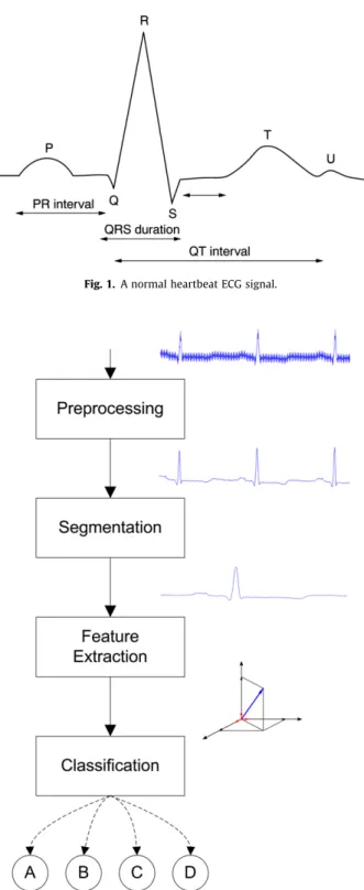
There are several methods proposed in the literature for the purpose of automatic arrhythmia classification in ECG signals, and a complete system for such an aim can be divided into four subsequent categories (preprocessing, segmentation, feature extraction, and classification) as shown inFig. 2, in which A, B, C and D illustrate fictitious heartbeat classes to be analyzed.
The preprocessing phase consists mainly in detecting and atten-uating frequencies of the ECG signal related to artifacts. Those arti-facts can be from a biological source, like muscular activity, or originated from an external source, such as 50/60 Hz electric net-work frequency. It is also desired, in the preprocessing, to perform a signal normalization and complex QRS (wave) enhancement (the most salient part of a heartbeat), in order to help the segmentation process.
0957-4174/$ - see front matterÓ2012 Elsevier Ltd. All rights reserved.
http://dx.doi.org/10.1016/j.eswa.2012.12.063
⇑ Corresponding author. Address: Universidade Federal de Ouro Preto, Computing Department, 35.400-000 Ouro Preto, MG, Brazil. Tel.: +55 31 3559 1692; fax: +55 31 3559 1660.
E-mail addresses:[email protected](Eduardo José da S. Luz), [email protected](T.M. Nunes),[email protected](Victor Hugo C. de Albuquerque),
[email protected](J.P. Papa),[email protected],[email protected](D. Me-notti).
Contents lists available atSciVerse ScienceDirect
Expert Systems with Applications
ECG signals segmentation consists in delimitating the part of the signal of more interest, the QRS complex, since it reflects the major part of the electrical activity of the heart (seeFig. 1). Once the segmentation of QRS complex is done one can obtain many physiological information, such as, for example, heart rate signal acquisition, in which will be used techniques to feature selection in order to eliminate redundant features from the primary feature set.
Feature extraction is the key point for the final classification performance. Features can be extracted directly from ECG wave-form morphology in time or frequency domain. Many
sophisti-cated computational methods have been considered in order to find features less sensitive to noise, such as the autoregressive model coefficients (Llamedo & Martı´nez, 2011), higher-order cumulant (higher order statistics) (Mehmet, 2004) and variations of wavelet transform (Addison, 2005; Özbay, 2009; Sayadi &
Sham-sollahi, 2007).
This work focuses mainly on the last step of cardiac arrhythmia analysis, i.e., ECG signal classification. A large number of ap-proaches have been proposed for this task, and the popular ones are statistical approaches based on Linear Discriminants (Chazal,
O’Dwyer, & Reilly, 2004), k-Nearest Neighbors (kNN) (Lanatá,
Val-enza, Mancuso, & Scilingo, 2011), Bayesian probabilities (Wiggins,
Saad, Litt, & Vachtsevanos, 2008), artificial neural networks (ANNs)
(Ceylan & Özbay, 2007; Korürek & Dogan, 2010; Özbay, 2009; Yu &
Chen, 2007; Yu & Chou, 2008), support vector machines (SVMs)
(Lin, Ying, Chen, & Lee, 2008b; Moavenian & Khorrami, 2010; Song,
Lee, Cho, Lee, & Yoo, 2005; Ye, Coimbra, & Kumar, 2010; Yu &
Choua, 2009), among others. We also find in the literature works
based on ECG signal clustering analysis (Ceylan, Özbay, & Karlik, 2009; Korürek & Nizam, 2008; Özbay, Ceylan, & Karlik, 2011;
Yeh, Chiou, & Lin, 2012), instead of classification. Once the
algo-rithm is run, the clusters are then manually or automatically classified.
However, according toChazal et al. (2004), Ince, Kiranyaz, and
Gabbouj (2009), Llamedo and Martı´nez (2011) few researchers
have used standard protocols to evaluate their expert system clas-sifiers, establishing learning and testing strategies with bias their results near the optimal ones (i.e., the perfect classification). Other works have considered not publicly available dataset (Özbay et al.,
2011; Yeh et al., 2012) which becomes difficult any kind of
com-parison. The majority of those researchers are favored by a biased training set (i.e., the heartbeats from the same patient are used for both training and testing the classifiers, which makes a fair com-parison among methods difficult) to train their classifiers. With such strategy, the classifiers know particularities of the patients’ heartbeat which is a non realistic situation. Usually the results of these works report effectiveness in average near 100% for heart-beats classification. When the constraint of heartbeat from the same patient in data division for training and testing classifiers is imposed, it noticeable that their achieved effectiveness drop a lot. These classification issues are intensively discussed on (Luz &
Menotti, 2011) showing that there is still to much room for
improvement.
In order to standardize comparison and overcome such difficul-ties,The Association for the Advancement of Medical Instrumentation (AAMI) has developed a standard (ANSI/AAMI/ISO EC57, 1998-R2008) for testing and reporting performance results of computa-tional techniques aiming at arrhythmia classification. The AAMI also recommends the use of the MIT-BIH Arrhythmia Database
(Mark & Moody, 1990) for performance evaluation of arrhythmia
systems. THE MIT-BIH Arrhythmia Database is the most widely used database for evaluation of the accuracy/sensitivity/specificity (from now on performance) of arrhythmia classification systems. This database was the first available for such a purpose and it has gone through several improvements over the years to encom-pass the broadest possible range of waveformsMoody and Mark
(2001). Here, we perform experiments following the AAMI
stan-dard and solely use the entire MIT-BIH Arrhythmia Database. In the context, a recent and powerful expert system classifier, proposed in Papa, Falcão, and Suzuki (2009)and customized in
Papa, Falcão, de Albuquerque, and Tavares (2012), named
opti-mum-path forest (OPF) classifier, arises for the automated detec-tion of specific problems and has been shown to be very effective, with excellent results compared to ANN and SVM (Papa
et al., 2009). The OPF classifier has been used in some applications
as, for example, petroleum well drilling monitoring (Guilherme Fig. 1.A normal heartbeat ECG signal.
et al., 2011), characterization of graphite particles in metallo-graphic images (Papa, Nakamura, de Albuquerque, Falcão, &
Tav-ares, 2013), classification of remote sensing images (Santos,
Gosselin, Philipp-Foliguet, Torres, & Falcão, 2012), nontechnical
losses detection (Ramos, Souza, Papa, & Falcão, 2011), segmenta-tion and classificasegmenta-tion of human intestinal parasites from micros-copy images Suzuki, Gomes, Falcão, Papa, and Shimizu (2012), among others, achieving promising results due to its advantages on other classifiers regarding efficiency (mainly computational cost), which is an important factor in ECG arrhythmia signal classi-fication. In the hospitals, the equipments used to accomplish the arrhythmia signal classification task, such as bed side monitors and defibrillators, often have limited resources. Despite of that OPF classifier has shown effectiveness compatible, and faster for training than other classifiers (Papa et al., 2012).
The aim of this work is to evaluate the OPF classifier perfor-mance focusing mainly on the last step of the cardiac arrhythmia analysis,i.e., ECG signal classification, considering mainly the com-putational cost, accuracy, sensitivity, and specificity. The perfor-mance is compared to the ones of three other well-known classifier algorithms widely used in the pattern recognition and machine learning literature (i.e, SVM with radial basis-function kernel, multi-layer perceptron neural network (MLP) and Bayesian expert system classifiers). Besides following the AAMI recommen-dation and using the MIT-BIH Arrhythmia Database for producing results reliable to clinic analysis, in order to perform our compari-son, on non normalized datasets, we re-implement six approaches
(Chazal et al., 2004; Güler & Übeyli, 2005; Song et al., 2005; Ye
et al., 2010; Yu & Chen, 2007; Yu & Chou, 2008) we consider quite
representative of the ECG signal feature extraction domain. These feature selection processes are reproduced as faithfully as possible to their description using Matlab. Each feature extraction set is then submitted to each considered expert system classifier.
The remainder of this work is organized as follows. The feature extraction approaches used in this work are briefly summarized in Section2. The OPF classifier and the other three expert system clas-sifiers are described in Section 3. The experimental results are shown in Section4, and discussed in Section5. Finally, in Section6, the conclusions are pointed out.
2. Feature extraction
In this section, the six feature extraction approaches used in this work for the comparison of classifiers are described. Observe that each approach comes from a work/paper which was used for arrhythmia classification, obviously using a classifier algorithm which is disregarded here. These approaches are chosen because they bring techniques widely used in literature and yet, the values of accuracy, sensitivity, sensibility reported are high compared to other published methods.
Notice that the six methods described here and used in our experiments and discussion are re-implemented as faithfully as possible to their description using Matlab.1
2.1. Chazal et al. (2004)
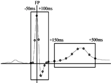
The most common feature found in the literature for ECG signal classification is computed from the cardiac rhythm (heartbeat interval) a.k.a. RR interval. The RR interval is the time between the heartbeat R peak (the most important fiducial point) regarding another R peak, which can be its predecessor or successor. InFig. 3, it is illustrated the RR interval and others also used in the
litera-ture. Except for patients who use pacemakers, the perceived varia-tions in the RR interval width are correlated with variavaria-tions in the morphology of the ECG signal curve, usually caused by arrhythmias
(Clifford, Azuaje, & McSharry, 2006). Features from the RR interval
reveal great discriminatory capabilities for heartbeat classes and have been used in several works in the literature, specially in
Cha-zal et al. (2004).
From the RR interval, we can extract four features which are used inChazal et al. (2004): the RR interval between the current and its predecessor heartbeat (RR-predecessor), the RR interval be-tween the current and its successor one (RR-posterior), the average of all RR interval containing in a full record (e.g., 30 min for in-stance) and also the average of ten RR interval around the current heartbeat.
Other features extracted from the cardiac beat intervals are also used in em (Chazal et al., 2004). These features are composed of distances between fiducial points in a heartbeat, as we can see in
Fig. 3. Among them, the QRS interval, or the QRS-complex duration,
is quite popular in the literature and also is use in (Chazal et al., 2004). Besides the length of QRS-complex, another time segment is used as feature in that work,i.e., the T wave length. The author also used the information about the presence/absence of P-wave. The algorithm used for fiducial point extraction in Chazal et al.
(2004)is proposed inLaguna, Jané, and Caminal (1994)and is also
used in this work here.
Nonetheless, the best classification results achieved in the liter-ature have used feliter-atures extracted from the RR interval and time segments of the heartbeat along with features extracted in the time/frequency domain (Chazal et al., 2004; Llamedo & Martı´nez, 2011). The simplest form to extract features in the time domain from the ECG signal curve is using its own sampled points as fea-tures (Wen, Lin, Chang, & Huang, 2009; Özbay & Tezel, 2010)
(seeFig. 4). However, using samples from the ECG curve as features
is not a such effective technique, due to both (1) the dimension of the feature vector produced is high (it depends on the amount of samples used to represent the heartbeat), (2) it suffers with several problems regarding scale and displacement related to the central point (the R peak). In order to decrease the feature vector size and avoid the aforementioned problems, inChazal et al. (2004), the authors used the interpolation of the ECG signal such that the final time representation is composed of 18 and 19 samples ob-tained from 250 samples (approximately 600 ms of curve/signal
Fig. 3. Fiducial points and important interval of a cardiac heartbeats. Extracted from (Clifford et al., 2006, Chapter 3).
initially sampled at 360 Hz – seeFig. 5). This process is applied in the two leads available in the dataset used. Then, for that work, a feature vector composed of the 52 best features reported is used.
2.2. Song et al. (2005)
InSong et al. (2005), instead of interpolating the ECG signal as
done inChazal et al. (2004), the authors used the wavelet trans-form to extract 15 features from the heartbeat. It is important to note that, the majority of works in the literature use the wavelet transform in the feature extraction process, because it allows the extraction of information in both time and frequency domain. Also, several works supports that this method is the best for feature extraction from ECG signals (Güler & Übeyli, 2005; Lin, Du, & Chen,
2008a; Mehmet, 2004).
In that work (Song et al., 2005), the heartbeat is represented as a 400 ms sampled window of the ECG signal centered at the R peak (144 samples). These samples are decomposed into seven levels using the wavelet transform, however only the detail coeffi-cients/sub-bands are used. Along with these feature, RR interval features (RR-predecessor and RR-posterior) are included in the fi-nal feature vector.
2.3. Güler and Übeyli (2005)
InGüler and Übeyli (2005), the authors also used the wavelet
transform to decompose the ECG signal (approximately 700 ms around the R peak) into 256 coefficients of the four first levels com-bining 247 from details and 18 from approximation sub-bands. In order to reduce the feature vector dimensionality, the authors used simple statistical measures: the average power, the mean, and the
standard deviation of the coefficients in each wavelet sub-band, and also the ratio of the absolute mean values of adjacent of sub-bands. The authors highlighted that the choice of the mother wave-let function used in the feature extraction process is critical to the final effectiveness of the classification. As a consequence of this claim, all the feature extraction processes using the wavelet trans-form studied in the work here were carefully reproduced taking into account the mother wavelet function suggested by the authors of each work.
2.4. Yu and Chen (2007)
In the work proposed inYu and Chen (2007), the authors used statistical techniques directly on heartbeat samples and, also, in three wavelet sub-bands: details of the first level of wavelet trans-form decomposition and approximation and details of the second level one. It is also used the AC power of the original signal, the AC power of each wavelet sub-band, the AC power of the autocor-relation function of the coefficients of each sub-band, and the ratio between the maximum and minimum values in each sub-band, adding up to 10 features. Besides these 10 statistical features, the authors also used the RR interval (RR-predecessor).
2.5. Yu and Chou (2008)
In Yu and Chou (2008), the independent component analysis
(ICA) is used to extract 100 coefficients from a heartbeat composed of 200 samples centered at the R peak. The ICA coefficients are computed using the Fast-ICA algorithm, proposed inHyvärinen
(1999), and only the first 33 coefficients are finally used. According
to the authors, the ICA is used to decompose the ECG signal in a weighted sum of the basic components which are mutually statis-tically independent. To these coefficients, the RR interval (RR-pre-decessor) is added.
2.6. Ye et al. (2010)
Ye et al. (2010)combined several feature extraction techniques
presented in the literature to generate their feature vector. Their features are extracted from 300 samples surrounding the R peak, being 100 before and 200 after the R peak. The wavelet transform is applied to the sampled ECG signal and 118 coefficients are ex-tracted from detail sub-bands of the third and fourth levels and approximation sub-band of the fourth level of the wavelet decom-position. Along with these features, eighteen coefficients extracted using the ICA (also using the algorithm proposed inHyvärinen
(1999)). This set of feature is named as morphological by the
authors.
Four features extracted from the RR interval, named as dynam-ical by the authors, are also used: RR-predecessor, RR-posterior, the average of all RR intervals of a record of a patient, and the aver-age of the 10 RR intervals surrounding (and centered to) the cur-rent heartbeat. In order to reduce the dimension of the obtained morphological feature vector to 26, the authors employed the prin-cipal components analysis (PCA) technique. This process is applied to the two ECG leads available on the MIT-BIH heartbeat record dataset, producing a final feature vector in which its dimension is twice than for a single lead.
3. Expert system classifiers
In this section, the four learning algorithms used in our compar-ison are presented. Special attention is given to the OPF classifier since to the best of our knowledge it is the first time that such algo-rithm is used for arrhythmia classification in ECG signals.
Fig. 4.ECG signal extracted from MIT-BIH AR database, sampled at 360 Hz.
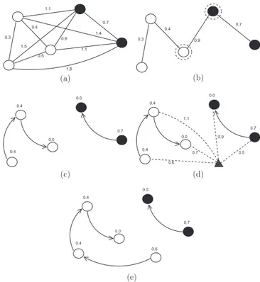
3.1. Optimum-path forest classifier
The optimum-path forest (OPF) is a framework to the design of pattern classifiers based on optimal graph partitionsPapa et al.
(2009, 2012), in which each sample is represented as a node of a
complete graph, and the arcs between them are weighted by the distance of their corresponding feature vectors. The idea behind OPF is to rule a competition process between some key samples (prototypes) in order to partition the graph into optimum-path trees (OPTs), which will be rooted at each prototype. We have that samples that belong to the same OPT are more strongly connected to their root (prototype) than to any other one in the optimum-path forest. Prototypes assign their costs (i.e., their lowest weight path or the maximum arc-weight along a path) for each node, and the prototype that offered the optimum path-cost will conquer that node, which will be marked with the same prototype’s label. LetZ=Z1[Z2be a dataset labeled with a functionk, in whichZ1 andZ2are, respectively, a training and test sets such thatZ1is used to train a given classifier andZ2is used to assess its accuracy. Let S#Z1a set of prototype samples. Essentially, the OPF classifier creates a discrete optimal partition of the feature space such that any samples2Z2can be classified according to this partition. This partition is an optimum path forest (OPF) computed inRnby the image foresting transform (IFT) algorithm (Falcão, Stolfi, & Lotufo,
2004).
The OPF algorithm may be used with any smooth path-cost function which can group samples with similar properties (Falcão
et al., 2004). Particularly, we used the path-cost function fmax,
which is computed as follows:
fmaxðhsiÞ ¼
0 ifs2S;
þ1 otherwise;
fmaxð
p
hs;tiÞ ¼maxffmaxðp
Þ;dðs;tÞg; ð1Þin whichd(s,t) means the distance between samplessandt, and a path
p
is defined as a sequence of adjacent samples. In such a way, we have that fmax(p
) computes the maximum distance be-tween adjacent samples inp
, whenp
is not a trivial path.The OPF algorithm assigns one optimum pathP⁄(s) fromSto
every samples2Z1, forming an optimum path forestP(a function with no cycles which assigns to eachs2Z1nSits predecessorP(s) in P⁄(s) or a markernilwhens2S). Let R(s)2Sbe the root ofP⁄(s)
which can be reached fromP(s). The OPF algorithm computes for eachs2 Z1, the costC(s) ofP⁄(s), the labelL(s) =k(R(s)), and the predecessorP(s).
The OPF classifier is composed of two distinct phases: (i) train-ing and (ii) classification. The former step consists, essentially, in finding the prototypes and computing the optimum-path forest, which is the union of all OPTs rooted at each prototype. Then, we take a sample from the test sample, connect it to all samples of the optimum-path forest generated in the training phase and we evaluate which node offered the optimum path to it. Notice that this test sample is not permanently added to the training set,i.e., it is used only once. The next sections describe in details this procedure.
3.1.1. Training
We say thatS⁄is an optimum set of prototypes when the OPF
algorithm minimizes the classification errors for everys2Z1. S⁄ can be found by exploiting the theoretical relation between mini-mum-spanning tree (MST) and optimum-path tree forfmax(Allène,
Audibert, Couprie, Cousty, & Keriven, 2007). The training
essen-tially consists in findingS⁄and an OPF classifier rooted atS⁄.
By computing a MST in the complete graph (Z1,A) (Fig. 6a), we obtain a connected acyclic graph whose nodes are all samples of
Z1and the arcs are undirected and weighted by the distancesd be-tween adjacent samples (Fig. 6b). The spanning tree is optimum in the sense that the sum of its arc weights is minimum as compared to any other spanning tree in the complete graph.
Algorithm 1. OPF training algorithm
In the MST, every pair of samples is connected by a single path which is optimum according tofmax. That is, the minimum-span-ning tree contains one optimum-path tree for any selected root node. The optimum prototypes are the closest elements of the MST with different labels inZ1(i.e., elements that fall in the frontier of the classes).Algorithm 1implements the training procedure for OPF.
The time complexity for training ish(jZ1j2), due to the main (lines 7–15) and inner loops (lines 10–15) inAlgorithm 1, which runh(jZ1j) times each.
After that, we have a collection of OPTs, each one of them rooted at each prototype, as one can see inFig. 6c. This geometry of the feature space gives the name to the classifier.
3.1.2. Classification
For any samplet2Z2, we consider all arcs connectingt with samples s2Z1, as though t were part of the training graph
(Fig. 6d). Considering all possible paths fromS⁄tot, we find the
optimum pathP⁄(t) from S⁄and labelt with the class k(R(t)) of
its most strongly connected prototypeR(t)2S⁄. This path can be
identified incrementally by evaluating the optimum costC(t) as
CðtÞ ¼minfmaxfCðsÞ;dðs;tÞgg;
8
s2Z1: ð2ÞLet the nodes⁄2Z
1be the one that satisfies Eq.(2)(i.e., the pre-decessorP(t) in the optimum pathP⁄(t)). Given thatL(s⁄) =k(R(t)),
the classification simply assignsL(s⁄) as the class oft(Fig. 6e). An
Algorithm 2. OPF classification algorithm
InAlgorithm 2, the main loop (lines 1–9) performs the
classifi-cation of all nodes inZ2. The inner loop (lines 4–9) visits each node kiþ12Z01; i¼1;2;. . .; Z01
1 until an optimum path
p
kiþ1 hkiþ1;ti is found.3.2. Bayesian classifier
Letp(
x
i—x) be the probability of a given patternx2Rnto be-long to classx
i,i= 1, 2,. . .,c, which can be defined by the BayesTheorem (Jaynes, 2003):
pð
x
ijxÞ ¼pðxjx
iÞPðx
iÞpðxÞ ; ð3Þ
wherep(xj
x
i) is the probability density function of the patterns that compose the classx
i, andP(x
i) corresponds to the probability of the classx
iitself.A Bayesian classifier decides whether a patternxbelongs to the class
x
iwhen:pð
x
ijxÞ>pðx
jjxÞ; i;j¼1;2;. . .;c; i–j; ð4Þwhich can be rewritten as follows by using Eq.(3):
pðxj
x
iÞPðx
iÞ>pðxjx
jÞPðx
jÞ; i;j¼1;2;. . .;x; i–j: ð5ÞAs one can see, the Bayes classifier´s decision functiondi(x) = p(xj
x
i)P(x
i) of a given classx
istrongly depends on the previous knowledge ofp(xjx
i) andP(x
i),"i= 1, 2,. . .,c. The probabilityval-ues ofP(
x
i) are straightforward and can be obtained by calculating the histogram of the classes. However, the main problem is to find the probability density functionp(xjx
i), given that the only infor-mation available is a set of patterns and its corresponding labels. A common practice is to assume that the probability density func-tions are Gaussian ones, and thus one can estimate their parame-ters using the dataset samples (Duda, Hart, & Stork, 2000). In the n-dimensional case, a Gaussian density of the patterns from classx
ican be calculated using:pðxj
x
iÞ ¼ 1ð2
p
Þn=2jCij1=2exp 1
2ðx
l
iÞ TC1i ðx
l
iÞ
; ð6Þ
in which
l
iandCicorrespond to the mean and the covariance ma-trix of classx
i. These parameters can be obtained by considering each pattern x that belongs to classx
i using the following equations:l
i¼1 NiX
x2xi
x; ð7Þ
and
Ci¼1
Ni
X
x2xi
xxT
l
i
l
Ti
; ð8Þ
in whichNimeans the number of samples from class
x
i.3.3. Support vector machines classifier
One of the fundamental problems of the learning theory can be stated as: given two classes of known objects, assign one of them to a new unknown object. Thus, the objective in a two-class pat-tern recognition is to infer a function (Schölkopf & Smola, 2002):
f:X! f1g; ð9Þ
regarding the input–output of the training data.
Based on the principle ofstructural risk minimization (Vapnik, 1999), the SVM optimization process is aimed at establishing a separating function while accomplishing the trade-off that exists between generalization and over-fitting.
Vapnik (1999)considered the class of hyperplanes in some dot
product spaceH,
hw;xi þb¼0; ð10Þ
wherew;x2H;b2R, corresponding to decision function:
fðxÞ ¼sgnðhw;xi þbÞ; ð11Þ
and, based on the following two arguments, the author proposed theGeneralized Portraitlearning algorithm for problems which are separable by hyperplanes:
1. Among all hyperplanes separating the data, there exists a uniqueoptimal hyperplanedistinguished by the maximum mar-gin of separation between any training point and the hyperplane.
2. The over-fitting of the separating hyperplanes decreases with increasing margin.
Thus, to construct the optimal hyperplane, it is necessary to solve:
minimize
w2H;b2R
s
ðwÞ ¼ 1 2kwk2
; ð12Þ
subject to:
yiðhw;xii þbÞP1 for all i¼1;. . .;m; ð13Þ
with the constraint(13)ensuring thatf(xi) will be +1 foryi= +1 and 1 foryi=1, and also fixing the scale ofw. A detailed discussion of these arguments is provided bySchölkopf and Smola (2002).
The function
s
in(12)is called theobjective function, while in (13) the functions are the inequality constraints. Together, they form a so-calledconstrained optimization problem. The separating function is then a weighted combination of elements of the train-ing set. These elements are calledsupport vectorsand characterize the boundary between the two classes.The replacement referred to as the kernel trick (Schölkopf &
Smola, 2002) is used to extend the concept of hyperplane
classifi-ers to nonlinear support vector machines. However, even with the advantage of ‘‘kernelizing’’ the problem, the separating hyperplane may still not exist.
In order to allow some examples to violate(13), the slack vari-ablesnP0 are introduced (Schölkopf & Smola, 2002), which leads to the constraints:
yiðhw;xii þbÞP1ni for all i¼1;. . .;m: ð14Þ
A classifier that generalizes efficiently is then found by control-ling both the margin (throughkwk) and the sum of the slack vari-ablesP
ini. As a result, a possible accomplishment of such asoft marginclassifier is obtained by minimizing the objective function:
s
ðw;nÞ ¼12kwk 2
þCXm
i¼1
ni; ð15Þ
subject to the constraint in(14), where the constantC > 0 deter-mines the balance between over-fitting and generalization. Due to the tuning variableC, these kinds of SVM based classifiers are nor-mally referred to as C-Support Vector Classifiers (C-SVC) (Cortes &
Vapnik, 1995).
3.4. Multi-layer perceptron neural network classifier
In this work we used an multi-layer perceptron neural networks (ANN-MLP) from fast artificial neural network library (FANN), in
Nissen (2003), which is a free open source ANN library, which
implements ANN-MLP in C and supports both fully and sparsely connected networks. The ANN-MLP is a combination of Perceptron layers aiming to solve multi-class problems Haykin (2007). The neural network architecture is composed of neuron layers, such that each output feeds the input neurons at the follows layer. The first layer, denoted byA, hasNA neurons, whereNAhas the same dimensionality of the feature vector, while the last layer, de-noted byQ, hasNQneurons, which stands for the number of the classes. This neural network assigns a pattern vectorxto a class
x
mif themth output neuron achieves the highest value.Each input layer corresponds to a weighted sum of the previous layer. LetJ1 be the previous layer ofJ, such that each inputIJ
jinJ is given by
IJ j¼
X
NK
k¼1
wjkOJk1 ð16Þ
and
OJ1
k ¼/ I J1
k
; ð17Þ
wherej= 1, 2,. . .,NJ, beingNJandNKthe amount of neurons at the layerJandJ1, respectively, andwjkstands for the weights that modify thekth output of layerJ1, i.e.,OJ1
k .
The backpropagation algorithm is usually employed to train MLP (Russell & Norvig, 2009). This algorithm minimizes the mean squared error between the desired outputsrqand the obtained out-putsUqof each node of the output layerQ. Therefore, the idea is to minimize the equation bellow:
EQ¼ 1
NQ
X
NQ
q¼1
ðrq
U
qÞ2; ð18Þin whichNQis the number of neurons at the output layerQ.
4. Experiments and results
In this work, we propose the use of a recent and powerful pat-tern recognition technique, the OPF classifier, for heartbeat ECG signal classification. In Section2, we surveyed six feature selection approaches widely used in the literature for this purpose, in which all were re-implemented. In Section3, we described the OPF clas-sifier along with the other three clasclas-sifiers, i.e., SVM, MLP, and Bayesian, which will be used in our experiments presented in this section. These features extraction approaches and classifier algo-rithms are combined to yield intelligent systems with high accu-racy and low computational cost.
The experiments works as follows. Initially we describe the dataset used, the suggested recommendations by the AAMI stan-dards to analyze and classify cardiac arrhythmia using ECG signals which recommends, and, finally, an explanation on how the MIT-BIH Arrhythmia Dataset is divided for creating the training (denominated in this work as DS1) and testing (denominated of DS2) sets as suggested inChazal et al. (2004). After, we present the measures used to evaluate the effectiveness of the expert sys-tem classifiers proposed in this work.
4.1. Database description and AAMI standards
values achieved by the AAMI F class in the works reported in the literature (Chazal et al., 2004; Llamedo & Martı´nez, 2011; Mar,
Zaunseder, Martínez, Llamedo, & Poll, 2011) and also in this work.
Also observe that the N AAMI class is dominant representing 89.46% of all heartbeats’ dataset. So attention has to be given in the effectiveness analysis of the results related to N AAMI class, since an optimal performance in only in that class means a final accuracy of almost 90%. Sensibility and specificity are measures that can capture the effectiveness performance of each class and are explained further in this section.
The AAMI standards also recommend dividing the recordings into two datasets: one for training and another for testing such that heartbeats from one recording (patient) are not used simulta-neously for both training and testing the classifier. As claimed be-fore and shown inLuz and Menotti (2011), when this constraint is not imposed for building the datasets for training and testing the classifiers achieve very high performance. However, such practice is not valid for considering realistic clinical results, since the clas-sifier is not trained with the data heartbeat of a patient to be ana-lyzed. Usually the heartbeats of a new patient does not belong to the training set, requiring the use of expert system classifiers more robust.
Then train (DS1) and test (DS2) sets are created, in order to accomplish AAMI recommendations and approximate to real world situation. As one can see from the values inTable 2an effort to bal-ance the amount of samples/heartbeat per class in the datasets is also noticed in such division. Note that #Rec stands for the number of records (patients) and DS1 and DS2 are suggested inChazal et al.
(2004)and not in ANSI/AAMI EC57:1998/(R)2008 standardAAMI
(2008). Moreover, analyzing the experiments performed on the
six works we studied here used for collect their feature representa-tion (presented in Secrepresenta-tion2), (Chazal et al., 2004) is the one to fol-lows the AAMI standards, while the others use different heartbeats of a same patient to be used in training and testing due to the high effectiveness they report in their works. This claim is show inLuz
and Menotti (2011).
The two partitions should be composed of the records of pa-tients’ heartbeats shown inTable 3, in which the numbers indicate a code for the recording of 30 min of heartbeat of each patient.
Chazal et al. (2004)claims that the record numbered 1## and
2## belongs to two class of patients (Mark & Moody, 1990),i.e. the first range are intended to serve as a representative sample of routine clinical recordings, while the second one contains com-plex ventricular, junctional, and supraventricular arrhythmias, so they decided to balance the presence of these records in each set such that the classifier has the larger diversity as possible for both training and testing, making these datasets the less biased as possible.
Observe that in such data division scheme heartbeats of a same patient are not present in both datasets, complying to the AAMI standards. That means that the heartbearts of a same patient are solely used to either (and not both) train or test the systems. The reasons for this constraint is to report the predictive effectiveness of ECG signal classification systems compatible in a real clinical trial.
All composition of feature extraction approaches and classifier algorithms are training in DS1 dataset and tested in DS2 following the scheme proposed inChazal et al. (2004).
4.2. Performance evaluation measures
In order to analyze the expert system classifiers, we present the three measures employed: accuracy, sensitivity, and specificity.
Accuracy (Acc) is defined as the ratio of total beats correctly classified and the number of total beats,
Accuracy¼beats correctly classified
number of total beats : ð19Þ
Sensitivity (Se) can be defined as the ratio of correctly classified beats of one class and the total beats classified as that class, includ-ing the missed classification beats,
Sensiti
v
ity¼ true positiv
estrue positi
v
esþfalse negativ
es ð20Þin whichtrue positivesandfalse negativesstand for the number of heartbeats of a given class correctly and incorrectly classified, respectively.
Table 1
Mapping the MIT-BIH Arrhythmia types to the AAMI classes.
The AAMI heartbeat class
N SVEB VEB F Q
Description Any heartbeat not in the S, V, F, or Q class
Supraventricular ectopic beat
Ventricular ectopic beat Fusion beat Unknown beat
MIT-BIH heartbeat types (code)
Normal beat (N) Atrial premature beat (A) Premature ventricular contraction (V)
Fusion of ventricular and normal beat (F)
Paced beat (P)
Left bundle branch block beat (L)
Aberrated atrial premature beat (a)
Ventricular escape beat (E)
Fusion of paced and normal beat (f) Right bundle branch block
beat (R)
Nodal (junctional) premature beat (J)
Unclassified beat (U)
Atrial escape beat (e) Supraventricular premature beat (S) Nodal (junctional) escape
beat (j)
Table 2
MIT-BIH Arrhythmia Dataset division scheme of the heartbeats.
Dataset N S V F Q Total #Rec
DS1 45,844 943 3788 415 8 50,998 22
DS2 44,238 1836 3221 388 7 49,690 22
Totals 90,082 2779 7009 803 15 100,688 44
Table 3
The division of records of patients’ heartbeats of the MIT-BIH Arrhythmia Dataset for training (DS1) and testing (DS2).
Record (patient number) of heartbeats
DS1 DS2
101 114 122 207 223 100 117 210 221 233
106 115 124 208 230 103 121 212 222 234
108 116 201 209 105 123 213 228
109 118 203 215 111 200 214 231
Specificity (Sp) stands for the ratio of correctly classified beats among all beats of a specific class,
Specificity¼ true negati
v
estrue negati
v
esþfalse positiv
es ð21Þin which true negativesstands for number of the heartbeats not belonging to a given class classified as not belonging to the consid-ered class, whilefalse positivesstands for the number of heartbeats incorrectly classified as belonging to a given class. Observe that these last two measures are based on the data of each class.
Furthermore, we also propose the use of a Harmonic mean (Hm) between sensitivity and specificity, mathematically express by:
HM¼2SeSp
SeþSp: ð22Þ
These measures can be computed from a confusion matrix which can be obtained by comparing the expected classification (reference data) which the ones predicted by a classifier.Table 4 shows in details how to compute these measures, obtained and firstly discussed byChazal et al. (2004). InTable 4(a) and (b), in dark gray (vertical highlighted lines), we illustrate how to compute the false positives for V and S AAMI classes, respectively, while in gray (horizontal highlighted lines), we illustrate how to compute the false negative for V and S AAMI classes, respectively. To com-puteSe’s eSp’s for N, F, and Q AAMI class we can proceed in a sim-ilar way to the ones of V and S AAMI classes.
Table 5
Training and testing time (in seconds) for MIT-BIH Arrhythmia Dataset following AAMI recommendations (5 classes).
Features Classifiers
SVM OPF Bayesian MLP
Train Test Total Train Test Total Train Test Total Train Test Total
Chazal et al. (2004) 192.92 181.08 374.00 609.71 895.78 1505. 49 90.79 2324.32 2415.11 3838.67 0.22 3838.89
Güler and Übeyli (2005) 078.01 059.99 138.00 216.69 220.87 0437.56 18. 80 0352.53 0371.33 1923.06 0.13 1923.19
Song et al. (2005) 095.07 057.75 152.81 205.64 229.02 0434.66 18. 24 0375.44 0393.68 1942.65 0.13 1942.78
Yu and Chen (2007) 107.38 069.65 177.02 250.40 222.31 0472.71 22. 80 0500.50 0523.29 2078.85 0.14 2078.99
Yu and Chou (2008) 066.00 049.02 115.01 187.80 176.81 0364.61 14. 47 0278.40 0292.87 1846.67 0.13 1846.80
Ye et al. (2010) 162.12 130.51 292.63 450.53 586.49 1037. 02 62.35 1572.71 1635.06 3083.42 0.18 3083.61
Table 6
Training and testing time (in seconds) for MIT-BIH Arrhythmia Dataset following the labeling suggestion fromLlamedo and Martı´nez (2011)(AAMI2-3 classes).
Features Classifiers
SVM OPF Bayesian MLP
Train Test Total Train Test Total Train Test Total Train Test Total
Chazal et al. (2004) 190.36 173.56 363.92 609.98 891.14 1501. 12 90.17 1393.75 1483.92 3682.04 0.21 3682.25
Güler and Übeyli (2005) 077.90 058.93 136.83 205.76 216.58 0422.34 18. 75 0209.50 0228.25 1790.11 0.13 1790.24
Song et al. (2005) 101.63 057.27 158.90 216.65 228.14 0444.78 18. 16 0226.17 0244.33 1794.33 0.13 1794.46
Yu and Chen (2007) 115.23 068.12 183.35 249.83 224.41 0474.24 22. 60 0302.08 0324.69 1947.38 0.14 1947.51
Yu and Chou (2008) 068.37 049.81 118.18 188.00 177.98 0365.98 14. 41 0168.84 0183.25 1700.25 0.12 1700.37
Ye et al. (2010) 158.11 129.90 288.02 443.63 581.69 1025. 32 62.24 0944.93 1007.17 2951.61 0.18 2951.78
Table 4
Computing the classifiers effectiveness from the confusion matrix. This scheme is extracted fromChazal et al. (2004)and adapted.
Although theaccuracyis the most important measure for decid-ing the choice of an expert system classifier, thesensitivity and specificity are measures quite important as well in this context, since the number of heartbeats for each class in the MIT-BIH Arrhythmia Database is very imbalanced and a single class (e.g., the normal beats) could represent most of the total accuracy, while the sensitivity and specificity directly depend on the number of samples for each class.
Besides these measures for evaluating and comparing the effec-tiveness performance of the expert system classifiers, we also com-pute the training and testingtime, which are also very important measures in ECG arrhythmia signal classification depending on the application.
5. Discussion
Our analysis and discussion of the results reported in this work are divided into two parts: efficiency and effectiveness. Note that all experiments reported here used a PC Intel i7 at 2.8 GHz and 4 Gb of RAM on a Linux Ubuntu operational system.
5.1. Efficiency
The run times obtained by the ECG signal expert system algo-rithms for learning the model from the entire training set (DS1) and for classifying the testing set (DS2) using the AAMI protocol (five classes) following the scheme proposed in Chazal et al.
(2004)and the AAMI protocol with the shorter groups of classes
(three classes) suggested byLlamedo and Martı´nez (2011)are re-ported inTables 5 and 6, respectively.
Regarding the training time, in average, the Bayesian classifiers achieved the best time, followed by the SVM classifier being in average almost four time slower than the Bayesian classifier. The OPF classifier presented the third best time being in average around 10 times greater than the one of the Bayesian classifier. In average, the MLP classifier is the slower one for learning the models, due to convergence criterion setup. However, the SVM classifier achieves the highest time for learning in two situations (both for the features extracted bySong et al. (2005)). It is impor-tant to note that the grid search time for the SVM’s
c
andC param-eters definitions are not taken into account in the training phase. It can be noticed that for the three classifiers, SVM, OPF and Bayesian, the changes in training time were not significant for 3 or 5 classes, but the MLP classifier obtained a significant training speed gain, reaching a time about 8% faster for three classes classification.Analyzing the testing time, due to its nature, as we can observe from these tables, the MLP classifier is the fastest one on the test set. Being four orders of magnitude slower, the SVM appears in sec-ond place for run on the testing data. The OPF classifier arises as the third fast one being in average one order of magnitude slower than SVM, and the slower classifier for the testing data in the most of the cases is the Bayesian classifier. It is important to note that only in three experiments (Table 6) the Bayesian classifier per-formed the testing task faster than the OPF classifier, due to the significant testing time decreasing caused by the reduction of the number of classes of the AAMI2 datasets. This reduction seem to affect most of all the Bayesian classifier speeding up its testing time up to 40%. Also observe that the testing time for the features extracted by Chazal et al. (2004)for all the classifiers is greater than to other features. This can be explained due to the higher vec-tor dimensionality of this feature representation.
Concerning the full run average time taken in our experiments, the SVM classifier is faster, being followed by the Bayesian, OPF and MLP classifiers. However, the time to define the parameters
cost (C) = 5 and Gamma (
c
) = 0.001 was not considered. These val- Tableues were reported in the literature inBhardwaj, Choudhary, and
Dayama (2012), in which is analyzed a graph between accuracy
and cost keeping gamma constant, and, further, accuracyv/s gam-ma keepingCconstant. When the parametrization of this values is considered in the train phase, the SVM classifier is much slower than the OPF and Bayesian classifiers, as can be seen in Papa et al. (2009), Guilherme et al. (2011), Papa et al. (2013), Santos
et al. (2012), Ramos et al. (2011), for example.
One can note that the Bayesian classifier was slower than OPF for two datasets, containing data of 5 classes extracted byChazal
et al. (2004) and Ye et al. (2010)due its high dimensional feature
vector. This statement is not true for three classes feature repre-sentations (datasets), where there is a speed gain in the testing time explained before.
5.2. Effectiveness
The effectiveness evaluation measures obtained, theAccuracy, Sensitivity, Specificity, and HM, by the ECG signal expert system algorithms trained on the training set (DS1) for classifying the test-ing set (DS2) containtest-ing 5 and 3 classes (similarly to the efficiency analysis) are shown inTables 7 and 8, respectively. Due to page width limits the floating points of the numbers in these table are omitted, and the figures in the tables represent percentages rang-ing from 000.0% to 100.0%.
As claimed before, the accuracy is the main important measure for analyzing the effectiveness of a ECG signal classification algo-rithm. Observing the accuracies values in Tables 7 and 8, it is noticeable that the SVM classifier obtained the highest accuracy in all feature representations used, regardless the amount of clas-ses in the training set (5 or 3), followed by MLP classifier, which ob-tained the second best performance also in all feature representations. OPF and Bayesian classifiers showed very close
performances, varying less then 0.4% and presenting together the worst overall accuracies.
Further in this section, it will be shown that most of the good accuracy obtained by SVM and MLP classifiers are due to a good performance only for the N class. This happens because the N class is the most representative class in the set, grouping more than 89% of the entire set.
As sensitivity and specificity of all classes take into account false negatives and positives, respectively, andHMis a combination of both, this parameter is an important one in our analysis of the capability of the method to differentiate the classes, and most of all the arrhythmic ones (S, V, V0, Q, and F). Due to this, we consider on our analysis these parameters.
A false negative for the N class means a false alarm, that is, the classifier detect an arrhythmic beat when its true class is normal, while a false positive for the N class means that an arrhythmic beat takes place and the classifier detect it as a normal beat. In some sit-uations, we prefer less false negatives (greater sensitivity than specificity) than false positives, and in other situations the oppo-site, that is why theHmanalysis is important which is defined as the harmonic mean of sensitivity and specificity to perform our analysis of the effectiveness in terms of sensitivity and specificity. Then, our analysis of the effectiveness for classes is concen-trated on the Harmonic mean values (Hm). Observing the values presented inTables 7 and 8, we can see that, despite of the best accuracy performance obtained by SVM and MLP classifiers, their performance as a differentiation tool between classes lacks effi-ciency. One can observe from the confusion matrices shown in
Ta-bles 9 and 10, from the worstHMfeature representation for SVM
classifier, in this caseYu and Chen (2007) and Song et al. (2005), respectively that this classifier, SVM, tends to fail on classifying samples for arrhythmic classes, prevailing the most numerous class, in this case the N class. This is a major problem, considering the purpose of the classification, where great part of the
arrhyth-Table 8
Accuracies, sensitivities and specificities (in 0.1%) for MIT-BIH Arrhythmia Dataset following the labeling suggestion fromLlamedo and Martı´nez (2011)(AAMI2-3 classes).
Features Classifiers
SVM OPF
Acc N S V0 Acc N S V0
Se/Sp/HM Se/Sp/HM Se/Sp/HM Se/Sp/HM Se/Sp/HM Se/Sp/HM
Chazal et al. (2004) 910 0979j360j526 0j1000j0 517j0978j677 810 845j537j657 010j971j020 773j880j823
Güler and Übeyli (2005) 895 0999j053j100 0j1000j0 080j0999j147 804 864j349j497 023j971j046 469j896j616
Song et al. (2005) 894 1000j031j060 0j1000j0 046j1000j087 814 848j658j741 183j954j306 722j888j796
Yu and Chen (2007) 890 1000j000j000 0j1000j0 000j1000j000 868 925j497j646 030j978j059 605j941j736
Yu and Chou (2008) 916 0998j257j409 0j1000j0 371j0997j541 909 957j593j732 177j988j300 700j963j811
Ye et al. (2010) 921 0998j329j495 0j1000j0 447j0994j617 895 932j618j743 121j994j216 824j938j877
Bayesian MLP
Chazal et al. (2004) 810 845j538j657 011j971j022 774j879j823 903 948j775j853 014j0993j028 792j929j855
Güler and Übeyli (2005) 803 863j350j498 023j972j046 471j894j617 893 981j184j310 001j0999j001 273j982j427
Song et al. (2005) 815 849j658j742 183j955j306 724j888j798 864 906j641j751 035j0985j067 768j911j834
Yu and Chen (2007) 871 928j495j645 027j978j053 605j943j737 887 957j332j493 002j1000j003 484j958j643
Yu and Chou (2008) 912 959j592j732 171j989j291 708j965j817 927 972j585j730 056j0993j106 819j977j891
Ye et al. (2010) 895 932j620j744 120j994j214 827j938j879 893 998j035j67 000j1000j000 053j998j100
Table 9
Confusion matrix for SVM classifying theYu and Chen (2007)dataset.
Class Algorithm
N S V F Q
True N 43905 0 0 0 0
S 01823 0 0 0 0
V 03197 0 0 0 0
F 00388 0 0 0 0
Q 00007 0 0 0 0
Table 10
Confusion matrix for SVM classifying theSong et al. (2005)dataset.
Class Algorithm
N S V F Q
True N 44212 0 006 0 0
S 01831 0 005 0 0
V 03064 0 155 0 0
F 00387 0 001 0 0
mic samples are classified as normal samples. This indicates that for this kind of classification, even with the best accuracy rates, the SVM classifier represents the worst result. The same analysis can be done for other feature representations and for three classes representations. It is clear also that the SVM classifier completely fails on classifying the S class, decreasing itsHMon all datasets tested.
In our analysis, we also observed that the same problem occurs with the MLP classifier, in a smaller degree, specially on classes S and F for most of the feature representations on both, 3 and 5 clas-ses analysis. On the other hand, we can note on the OPF and Bayes-ian classifiers HM results, a very much better performance, showing to be more robust, despite of their lower accuracy rates. Moreover, the results obtained by both are very similar, allowing us to say they have almost the same performance on classifying arrhythmic classes. This ability to evaluate samples provided by potential diseased patients and differentiate it is the most impor-tant in our analysis, due to the goal of the classification system in detecting possible heart diseases.
So, from these analyses we can conclude that the OPF and Bayesian classifiers produce similar results and the best balance among classification of normal and arrhythmic classes when com-pared to the SVM and MLP classifiers.
Observe that the effectiveness achieved for class Q inTable 7by the classifiers with all feature representations are negligible. The Q class almost always achieves zero value for sensitivity, leading to anHM0. The performance on classifying F class are also weak per-formances, than the other classes, due to its nature of being a fu-sion between two other classes. Due to the non representative amount of beats of class Q (less than 0.015% of the database) and to the difficult of the majority works in the literature and also those shown here in classifying the F class, the protocol called AAMI2 was proposed, in which the Q class was removed and the classes V and F class were fused into V0class. By observing the Har-monic mean values (Hm) for the V class inTable 7and V’ class in8, we can see that the fusion of V and F classes to V class does not im-pact the results for the V0and S classes when the OPF and Bayesian classifier are used. For SVM and MLP classifiers, there is an slightly impact but without leading to a better classification overall. This is a very important result for classification using Bayesian classifier, which was highly affected by the number of classes, in terms of speed. The problem with the number of classes, does not occur with the OPF classifier, since the training and testing time where not significantly affected, showing a great robustness of this classifier.
6. Conclusions
In this work, we investigated the use of the OPF classifier for the task of Arrhythmic ECG signal classification. To the best of our knowledge, it is the first that the OPF classifier is applied to ECG signal classification. Moreover, we studied and implemented six feature representation from works in the literature (Chazal et al., 2004; Güler & Übeyli, 2005; Song et al., 2005; Yu & Chen, 2007;
Yu & Chou, 2008; Ye et al., 2010) which in our opinion are quite
representative. Besides applying these feature representation ap-proaches to learn model with the OPF classifier, we also employ the use of other three well-know learning algorithms: support vec-tor machines, multi-layer perceptron neural network (MLP), and Bayesian expert system classifiers.
The experiments reported here shown that the MLP classifier is the fastest one for the testing task, while the learning task is best performed by the SVM classifier. Nonetheless, in average, the OPF classifier has shown an efficiency performance not being five times worst than SVM classifiers. On the other hand, the OPF classifier
to-gether with the Bayesian one have shown the best balance for clas-sifying the arrhythmic classes, despite the best accuracy performance yielded by the MLP and SVM classifier which biased the classification towards the normal class failing to classify the arrhythmic classes.
Acknowledgments
The first and last authors would like to thank FAPEMIG, CAPES, and CNPq for the financial support. The third author thank to CNPq and Cearense Foundation for the Support of Scientific and Techno-logical Development (FUNCAP) for providing financial support through a DCR Grant #35.0053/2011.1 to Universidade de Fort-aleza (UNIFOR). The forth author is grateful to National CNPq Grant #303182/2011-3, and FAPESP Grant #2009/16206-1.
References
Addison, P. S. (2005). Wavelet transforms and the ECG: A review.Physiological Measurement, 26(5), 155–199.
Allène, C., Audibert, J. Y., Couprie, M., Cousty, J., & Keriven, R. (2007). Some links between min-cuts, optimal spanning forests and watersheds. InMathematical morphology and its applications to image and signal processing, MCT/INPE(pp. 253–264).
Association for the Advancement of Medical Instrumentation (AAMI) (2008).Testing and reporting performance results of cardiac rhythm and ST segment measurement algorithms. American National Standards Institute, Inc. (ANSI), ANSI/AAMI/ISO EC57, 1998-(R)2008.
Bhardwaj, P., Choudhary, R. R., & Dayama, R. (2012). Analysis and classification of cardiac arrhythmia using ECG signals. International Journal of Computer Applications, 38(1), 37–40.
Ceylan, R., & Özbay, Y. (2007). Comparison of FCM, PCA and WT techniques for classification ECG arrhythmias using artificial neural network.Expert Systems with Applications, 33(2), 286–295.
Ceylan, R., Özbay, Y., & Karlik, B. (2009). A novel approach for classification of ECG arrhythmias: Type-2 fuzzy clustering neural network. Expert Systems with Applications, 36(3), 6721–6726.
Chazal, P., O’Dwyer, M., & Reilly, R. B. (2004). Automatic classification of heartbeats using ECG morphology and heartbeat interval features. IEEE Transactions on Biomedical Engineering, 51(7), 1196–1206.
Clifford, G. D., Azuaje, F., & McSharry, P. (2006).Advanced methods and tools for ECG data analysis(first ed.). Artech House Publishers.
Cortes, C., & Vapnik, V. (1995). Support vector networks.Machine Learning, 20(3), 273–297.
Duda, R. O., Hart, P. E., & Stork, D. G. (2000).Pattern classification. Wiley-Interscience Publication.
Falcão, A. X., Stolfi, J., & Lotufo, R. A. (2004). The image foresting transform theory, algorithms, and applications.IEEE Transactions on Pattern Analysis and Machine Intelligence, 26(1), 19–29.
Guilherme, I. R., Marana, A. N., Papa, J. P., Chiachia, G., Afonso, L. C. S., Miura, K., et al. (2011). Petroleum well drilling monitoring through cutting image analysis and artificial intelligence techniques.Engeneering Applications of Artficial Inteligence, 24, 201–207.
Güler, I., & Übeyli, E. D. (2005). ECG beat classifier designed by combined neural network model.Pattern Recognition, 38(2), 199–208.
Haykin, S. (2007).Neural networks: A comprehensive foundation(third ed.). Prentice-Hall, Inc.
Hyvärinen, A. (1999). Fast and robust fixed-point algorithms for independent component analysis.IEEE Transactions on Neural Networks, 10(3), 626–634. Ince, T., Kiranyaz, S., & Gabbouj, M. (2009). A generic and robust system for
automated patient-specific classification of ECG signals.IEEE Transactions on Biomedical Engineering, 56(5), 1415–1427.
Jaynes, E. T. (2003).Probability theory: The logic of science. Cambridge University Press.
Korürek, M., & Dogan, B. (2010). ECG beat classification using particle swarm optimization and radial basis function neural network.Expert Systems with Applications, 37(12), 7563–7569.
Korürek, M., & Nizam, A. (2008). A new arrhythmia clustering technique based on ant colony optimization.Journal of Biomedical Informatics, 41, 874–881. Laguna, P., Jané, R., & Caminal, P. (1994). Automatic detection of wave boundaries in
multilead ECG signals: Validation with the CSE database. Computers and Biomedical Research, 27(1), 45–60.
Lanatá, A., Valenza, G., Mancuso, C., & Scilingo, E. (2011). Robust multiple cardiac arrhythmia detection through bispectrum analysis. Expert Systems with Applications, 38(6), 6798–6804.
Lin, C., Du, Y., & Chen, T. (2008a). Adaptive wavelet network for multiple cardiac arrhythmias recognition.Expert Systems with Applications, 34(4), 2601–2611. Lin, S.-W., Ying, K.-C., Chen, S.-C., & Lee, Z.-J. (2008b). Particle swarm optimization
Llamedo, M., & Martínez, J. P. (2011). Heartbeat classification using feature selection driven by database generalization criteria. IEEE Transactions on Biomedical Engineering, 58(3), 616–625.
Luz, E., & Menotti, D. (2011). How the choice of samples for building arrhythmia classifiers impact their performances. In Engineering in Medicine and Biology Society (EMBC), annual international conference of the IEEE(pp. 4988–4991).
Mar, T., Zaunseder, S., Martínez, J. P., Llamedo, M., & Poll, R. (2011). Optimization of ECG classification by means of feature selection.IEEE Transactions on Biomedical Engineering, 58(8), 2168–2177.
Mark, R. G., & Moody, G. B. (1990). MIT-BIH ECG database. Available at<http:// ecg.mit.edu/dbinfo.html>.
Mehmet, E. (2004). ECG beat classification using neuro-fuzzy network.Pattern Recognition Letters, 25(15), 1715–1722.
Moavenian, M., & Khorrami, H. (2010). A qualitative comparison of artificial neural networks and support vector machines in ECG arrhythmias classification.Expert Systems with Applications, 37(4), 3088–3093.
Moody, G. B., & Mark, R. G. (2001). The impact of the MIT-BIH arrhythmia database. IEEE Engineering in Medicine and Biology Magazine, 20(3), 45–50.
Nissen, S. (2003).Implementation of a fast artificial neural network library (FANN). Department of Computer Science University of Copenhagen (DIKU). Software available at<http://leenissen.dk/fann/>.
Özbay, Y. (2009). A new approach to detection of ECG arrhythmias: Complex discrete wavelet transform based complex valued artificial neural network. Journal of Medical Systems, 33(6), 435–445.
Özbay, Y., Ceylan, R., & Karlik, B. (2011). Integration of type-2 fuzzy clustering and wavelet transform in a neural network based ECG classifier.Expert Systems with Applications, 38(1), 1004–1010.
Özbay, Y., & Tezel, G. (2010). A new method for classification of ECG arrhythmias using neural network with adaptive activation function. Digital Signal Processing, 20(4), 1040–1049.
Papa, J. P., Falcão, A. X., de Albuquerque, V. H. C., & Tavares, J. M. R. S. (2012). Efficient supervised optimum-path forest classification for large datasets. Pattern Recognition, 45(1), 512–520.
Papa, J. P., Falcão, A. X., & Suzuki, C. T. N. (2009). Supervised pattern classification based on optimum-path forest.International Journal of Imaging Systems and Technology, 19(2), 120–131.
Papa, J. P., Nakamura, R. Y. M., de Albuquerque, V. H. C., Falcão, A. X., & Tavares, J. M. R. S. (2013). Computer techniques towards the automatic characterization of graphite particles in metallographic images of industrial materials. Expert Systems with Applications 40(2), 590–597.
Ramos, C. C. O., Souza, A. N., Papa, J. P., & Falcão, A. (2011). A new approach for nontechnical losses detection based on optimum-path forest.IEEE Transactions on Power Systems, 26(1), 181–189.
Russell, S. J., & Norvig, P. (2009).Artificial intelligence: A modern approach(third ed.). Prentice-Hall.
Santos, J. A., Gosselin, P. H., Philipp-Foliguet, S., Torres, R. S., & Falcão, A. X. (2012). Multi-scale classification of remote sensing images. IEEE Transactions on Geoscience and Remote Sensing, 50(10), 3764–3775.
Sayadi, O., & Shamsollahi, M. B. (2007). Multiadaptive bionic wavelet transform: Application to ECG denoising and baseline wandering reduction. EURASIP Journal on Advances in Signal Processing, 2007(14), 1–11.
Schölkopf, B., & Smola, A. J. (2002).Learning with kernels. MIT Press.
Song, M. H., Lee, J., Cho, S. P., Lee, K. J., & Yoo, S. K. (2005). Support vector machine based arrhythmia classification using reduced features.International Journal of Control, Automation, and Systems, 3(4), 509–654.
Suzuki, C. T. N., Gomes, J. F., Falcão, A. X., Papa, J. P., & Shimizu, S. H. (in press). Automatic segmentation and classification of human intestinal parasites from microscopy images.IEEE Transactions on Biomedical Engineering.
University of Maryland Medical Center (2012). English medical encyclopedia. Available at<http://www.umm.edu/ency/>. Last accessed October 16th. Vapnik, V. N. (1999). An overview of statistical learning theory.IE EE Transactions on
Neural Networks, 10(5), 988–999.
Wen, C., Lin, T.-C., Chang, K.-C., & Huang, C.-H. (2009). Classification of ECG complexes using self-organizing CMAC.Measurement, 42(3), 399–407. Wiggins, M., Saad, A., Litt, B., & Vachtsevanos, G. (2008). Evolving a bayesian
classifier for ECG-based age classification in medical applications.Applied Soft Computing, 8(1), 599–608.
Ye, C., Coimbra, M. T., & Kumar, B. V. K. V. (2010). Arrhythmia detection and classification using morphological and dynamic features of ECG signals. InIEEE international conference on Engineering in Medicine and Biology Society (EMBC) (pp. 1918–1921).
Yeh, Y.-C., Chiou, C. W., & Lin, H.-J. (2012). Analyzing ECG for cardiac arrhythmia using cluster analysis.Expert Systems with Applications, 39(1), 1000–1010. Yu, S., & Chen, Y. (2007). Electrocardiogram beat classification based on wavelet
transformation and probabilistic neural network.Pattern Recognition Letters, 28(10), 1142–1150.
Yu, S., & Chou, K. (2008). Integration of independent component analysis and neural networks for ECG beat classification.Expert Systems with Applications, 34(4), 2841–2846.