ii
Paulo Guilherme Molin
ESTIMATION OF VEGETATION CARBON STOCK IN
ii
ESTIMATION OF VEGETATION CARBON STOCK IN PORTUGAL USING LAND USE / LAND COVER DATA
Dissertation supervised by Professor Mário Caetano, PhD
Dissertation co-supervised by Professor Marco Painho, PhD
Professor Filiberto Pla, PhD
iii
ACKNOWLEDGMENTS
I would like to sincerely thank my supervisor Prof. Dr. Mario Caetano, for his exceptional supervision and guidance as well as for the invaluable suggestions and opportunities given to me by him. I would also like to thank Prof. Dr. Marco Painho and Prof. Dr. Filiberto Pla, for their co-supervision in this study.
I would like to express my gratitude towards the European Commission (Erasmus Mundus Program) MSc in Geospatial Technologies consortium for providing the opportunity and financial means of pursuing my studies in Europe. A special thanks to all my friends and classmates who have also been experiencing this opportunity for the last 18 months.
To all faculty members and staff from New University of Lisbon, University of Muenster, and University of Jaume I, I thank you. I am especially thankful for the assistance and cooperation of Prof. Dr. Werner Kuhn, Prof. Dr. Christoph Brox, Prof. Dr. Marco Painho and Prof. Dr. Mário Caetano that along with the help of staff members and friends such as Maria do Carmo, Paulo Sousa, Caroline Wahle and Angela Santos have helped me throughout my stay in Lisbon and Muenster.
I would like to express my sincere thanks to Maria Conceição Pereira, Hugo Carrão and Antonio Nunes from IGP for their help providing data and ideas for this study.
iv
ESTIMATION OF VEGETATION CARBON STOCK IN PORTUGAL USING LAND USE / LAND COVER DATA
ABSTRACT
v
ESTIMATIVA DE STOCK DE CARBONO NA VEGETAÇÃO DE PORTUGAL
UTILIZANDO DADOS DE USO E OCUPAÇÃO DO SOLO
RESUMO
vi KEYWORDS
Carbon Stock CORINE Land Cover Land Use / Land Cover Minimum Mapping Unit Scale
PALAVRAS CHAVES
CORINE Land Cover Escala
Stock de Carbono
vii ACRONYMS
CA – Combine & Assign
CAOP – Carta Administrativa Oficial de Portugal (Portuguese Official Administrative Cartography)
CDM – Clean Development Mechanism CFC – Chlorofluorocarbon
CLC – CORINE Land Cover
COS – Carta de Ocupação do Solo de Portugal (Portuguese Land Use Cartography)
CORINE – Coordination of Information on the Environment DR – Direct Remote Sensing
EEA – European Environmental Agency EIT – Economies in Transitions
EU – European Union GHG – Green House Gases
GIS – Geographical Information System
IGP – Instituto Geográfico Português (Portuguese Geography Institute) IPCC – Intergovernmental Panel on Climate Change
LIDAR – Light Detection and Ranging LULC – Land Use / Land Cover
LULUCF – Land Use, Land Use Change and Forestry MMU – Minimum Mapping Unit
NUTS – Nomenclature of Territorial Units for Statistics
OECD – Organization for Economic Co-operation and Development RADAR – Radio Detection and Ranging
SAR – Synthetic Aperture RADAR SM – Stratify & Multiply
viii
TABLE OF CONTENTS
ACKNOWLEDGMENTS ... iii
ABSTRACT ...iv
RESUMO ... v
KEYWORDS ...vi
ACRONYMS ... vii
TABLE OF CONTENTS ... viii
INDEX OF TABLES ... x
INDEX OF FIGURES ... xi
1. INTRODUCTION ... 1
1.1 Background ...2
1.1.1 Climate Change ...2
1.1.2 Carbon Cycle ...4
1.1.3 Kyoto Protocol ...5
1.2 Problem Statement ...7
1.3 Research Questions ...8
1.4 Objectives ...8
1.5 Hypotheses ...8
1.6 Study Area ...8
1.7 Overview of Document ... 11
2. REMOTE SENSING AND GIS AS TOOLS FOR CARBON STOCK MONITORING ... 13
2.1 Remote Sensing ... 13
2.2 Land Use /Land Cover ... 15
2.3 Geographic Information Systems ... 16
2.3.1 Scale ... 17
2.4 Vegetation Carbon Stock Studies ... 18
2.5 Conclusions ... 22
3. MATERIALS AND METHODS ... 23
3.1 Materials ... 23
3.1.1 Data ... 23
3.1.2 Software ... 30
3.2 Methods ... 31
3.2.1 Carbon Stock Estimation Using CORINE Land Cover ... 31
ix
3.3 Summary ... 37
4. RESULTS AND DISCUSSION ... 38
4.1 Vegetation Carbon Stock Estimation Using CORINE Land Cover ... 38
4.2 The Effect of Scale (MMU) On Vegetation Carbon Stock Estimation ... 46
4.3 Summary ... 50
5. CONCLUSIONS ... 52
5.1 Discussion on Research Questions ... 53
5.2 Discussion on Hypothesis ... 54
5.3 Recommendations ... 54
5.4 Limitations and Future Studies... 55
BIBLIOGRAPHIC REFERENCES ... 56
APPENDICES ... 60
1. Details on Carbon Density Values (Cruickshank et al., 2000) ... 61
2. Summary Tables for the Vegetation Carbon Stock Study of Continental Portugal ... 64
x INDEX OF TABLES
xi
INDEX OF FIGURES
xii
Figure 18: Distribution of vegetation carbon stock of each Mega Class per year
... 42
Figure 19: Spatial distribution representation of the vegetation carbon stock of Continental Portugal for three years ... 43
Figure 20: Vegetation carbon stock change detection over three periods ... 44
Figure 21: Distribution of vegetation carbon stock for each NUTS II administrative division over each of the three years studied ... 45
Figure 22: Distribution of carbon stock throughout different MMUs with addition of a linear trendline ... 46
Figure 23: Vegetation carbon stock for each MMU of Castro Verde study area . 47 Figure 24: Area size for each MMU of Castro Verde study site ... 47
Figure 25: Vegetation carbon stock for each MMU of Nelas study site ... 48
Figure 26: Area size for each MMU of Nelas study site ... 48
Figure 27: Vegetation carbon stock for each MMU of Mora study site ... 49
1
1. INTRODUCTION
Global climate is being affected and changed by natural and human activities. The climate change which is resulting from human activities is linked to the emission of greenhouse gases (GHG) into the atmosphere. Gases such as carbon dioxide (CO2), methane (CH4) and chlorofluorocarbon (CFC) contribute to global warming. A widely discussed strategy to reduce GHGs, especially CO2, with great potential of success is the use of forests and other vegetation to sequester carbon from the atmosphere (Watson, Zinyowera et al. 1996; Paustian, Cole et al. 1998; Holly, Martin 2007; Valsta, Lippke et al. 2008).
Vegetation, especially forests, are known for accumulating different amounts of carbon, depending on species and its geographic location. The possibility of using vegetation as carbon reservoirs has been identified as a potential measure to mitigate the GHGs effect of global warming. The accumulation of carbon by the vegetation is defined generally as a mean of “Carbon Stock”. This stock is present in all living materials, from leafs, to stems, barks, roots and microbial biomass, but is also present in dead material such as litter and organic carbon in the soil (Watson, Zinyowera et al. 1996; Amézquita, Ibrahim et al. 2005; Orrego 2005).
2
increase or decrease of carbon stock (Ruimy, Saugier et al. 1994; Jensen 2000; Franklin 2001; Melesse, Weng et al. 2007; Mäkipää, Lehtonen et al. 2008; Maselli, Chiesi et al. 2008).
1.1Background
1.1.1 Climate Change
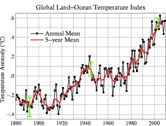
Climate change can be defined as a change in the circulation of weather throughout a specific region or in a global perspective. This change occurs over a period of time that can range from decades to millions of years. In the context of environmental policies, climate change is referred to as a change in modern climate or even used as a synonym to “global warming” (Figure 1). As for the United Nations Framework Convention on Climate Change (UNFCCC), climate change means “a change of climate which is attributed directly or indirectly to human activity that alters the composition of the global atmosphere and which is in addition to natural climate variability observed over comparable time periods” (UN 1992).
Figure 1: Plot of global annual-mean surface air temperature change derived from the meteorological station network (Source: NASA 2010b)
3
deformation of Earth’s crust, continental drift and changes in concentration of GHGs. Supposedly, the last one is the only factor where man has any influence, either in benefit or detriment of.
According to many international scientific studies, human activities resulted in substantial global warming from the 20th century onwards. Human induced emissions of GHG continued to grow generating high risks of climate change. Predictions from the Intergovernmental Panel on Climate Change (IPCC) show that an average rise in temperature in a global scale will be of between 1.4ºC and 5.8ºC for the period of 1990 and 2100 (Houghton, Ding et al. 2001).
The relation between carbon and global warming is due to the greenhouse effect that CO2 naturally has on Earth. The temperature of Earth is the subtraction of the energy coming from the Sun from the energy that is bounced back into outer space. Carbon in the atmosphere acts as a shield to the heat energy bouncing back from Earth and is in fact a benefit because it preserves a balance in the temperature. The problems is that higher concentration of carbon in the atmosphere (Figure 2) is strongly correlated to higher average temperatures in the Earth (Petit, Jouzel et al. 1999).
4 1.1.2 Carbon Cycle
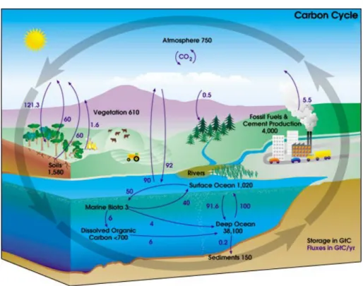
This biogeochemical called carbon is found in four major reservoirs or pools which are interconnected in a way to form the cycle. The four major pools of carbon are the atmosphere, ocean, sediments and terrestrial biosphere. Considered as one of the most important cycles on Earth, carbon cycle is an exchange of carbon among the four pools. This cycle permits the carbon element to be recycled and reused by the biosphere (Falkowski, Scholes et al. 2000).
The annual exchange and movement of the element are related to chemical, physical, geological and biological processes. An analysis of the exchanges reveals the incomes and outflows between each pool resulting in a final global carbon budget (Figure 3). A further examination of the budget would inform whether the pool functions as a source or sink for the element. In the biosphere, carbon can be stored for hundreds of years in trees and up to thousands of years in soils making both very important and interesting long term carbon pool. The threat of deforestation and its consequences to the soil make it also one of the major hazards to climate change influenced by man (Schimel 1995).
Figure 3: Carbon cycle diagram showing storage and annual exchange of carbon between atmosphere, hydrosphere and geosphere in gigatons of Carbon (Gt) (Source:
5 1.1.3 Kyoto Protocol
In December 11, 1997, during the UNFCCC, a Protocol was adopted aimed at combating global warming. This international treaty, which entered into force on February 16, 2005, had the objective of stabilizing GHG concentrations in the atmosphere in order to prevent hazardous interference with climate system. The Kyoto Protocol is an international agreement that has set a goal that from the year 2008 till 2012 the industrialized countries would reduce their GHG emissions by five percent compared to their 1990 rates. Failure to meet the targeted goal could compel a country to stop some of its industrial production, setting back its economies (Grubb, Vrolijk et al. 1999).
As of November 6, 2009, 189 countries and 1 regional economic integration organization have deposited instruments of ratification, accession, approval or acceptance to the referred Protocol. In a special composition of the Protocol there are 41 industrialized countries identified as “Annex I” countries which committed themselves to the reduction of 5.2% of GHG by the year 2012 – compared to what was produced by them in 1990.
The Annex I is composed of 41 countries that include the industrialized countries that were members of the Organization for Economic Co-operation and Development (OECD) in 1992, plus countries with economies in transition (the EIT Parties), including the Russian Federation, the Baltic States, and several Central and Eastern European States (UNFCCC 2009). Each of these countries, which includes Portugal and other European Union (EU) members, are required to submit annual reports accounting inventories of any anthropogenic GHG emission from sources or removals from sinks under the UNFCCC and Kyoto Protocol (UNFCCC 2010).
The Kyoto Protocol gave way to flexible mechanisms such as emission trading, clean development mechanism (CDM) and other implementation strategies which in return allow the Annex I countries to meet their GHG commitments. This allowed states to buy GHG emission reductions credits (also referred to as carbon credits) from other states (Grubb, Vrolijk et al. 1999).
6
policies and measures to reduce the GHGs such as through carbon sequestration. Third, establish adaptation funds for climate change in developing countries through which impacts could be minimized. Fourth, compliance by establishing a committee to enforce agreements and at last the fifth which is to account, report and review to ensure the integrity of the Kyoto Protocol (Freestone, Streck 2007).
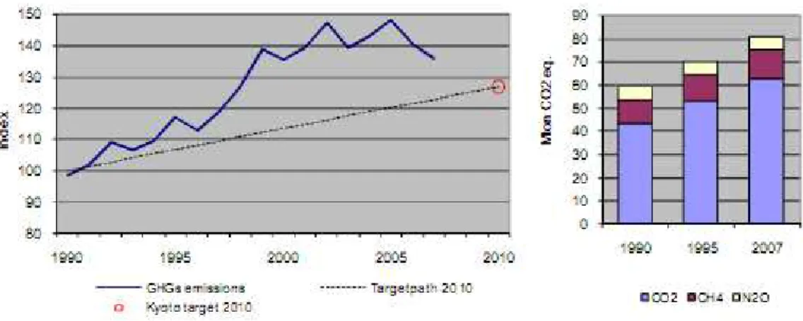
The EU has made a joint reduction goal of 8% in relation to its emissions in 1990. For Portugal, this means that it must also reduce its emissions by 8% even though it represented only 0.3% of emissions generated by the total Annex 1 parties in 1990. Under the EU burden sharing agreement Portugal is committed to limiting its emissions during the first commitment period to no more than +27% compared to the 1990 level. The Portuguese National Inventory Report on Greenhouse Gases, 1990-2007 Submitted under the United Nations Framework Convention on Climate Change and the Kyoto Protocol (Pereira, Seabra et al. 2009) has reported that Portugal has emitted 36% more GHG in 2007 than in 1990, without counting Land Use, Land Use Change and Forestry (LULUCF). Remembering that in the first commitment period Portugal was set to limit its emissions by +27% until 2010 and therefore emissions were in 2007 above the target path (Figure 4).
7
Figure 4: GHG emissions for Portugal without LULUCF (Source: Pereira, Seabra et al. 2009)
1.2 Problem Statement
This study describes an effort to estimate vegetation carbon stock in Continental Portugal using CORINE (Coordination of Information on the Environment) land cover (CLC). These LULC are maps derived from remote sensed images and are characterized by having a minimum mapping unit (MMU) of 25 ha. By means of measuring carbon stock on vegetation cover derived from CLC90 (year 1985), CLC00 (year 2000) and CLC06 (year 2006), and the addition of different vegetation carbon densities gathered in literature, it was possible to produce high-quality estimates of carbon stock for the continental part of the country as well as identify its spatial distribution and carbon change detection.
An interesting approach of this study is the possibility of encouraging the use of CLC for carbon stock estimates to verify international carbon reduction agreements not only by Portugal but also by other countries that develop and use CLC maps.
8 1.3 Research Questions
This research was considered and implemented in a way to answer the following questions:
1) What are the total carbon stocks of Portugal for the years 1985, 2000 and 2006?
2) What are the statistical differences in each year and to each class? 3) What is the spatial distribution of carbon throughout Portugal? 4) How does the MMU effect carbon stock estimation?
1.4 Objectives
The research undertaken intends to quantify the carbon stocks of Portugal for the years 1990, 2000 and 2006 as well as to consider the effects of MMU in its calculation.
A list of more specific objectives for this study can be listed below: Identify optimum carbon density values for each CLC class; Assess the carbon stock of Portugal for each of the CLC datasets; Analyze results;
Produce maps of spatial distribution of carbon stock of Portugal; and Produce a diverse quantity of maps with diverse values of MMU to
analyze its effects on carbon stock. 1.5 Hypotheses
The following hypotheses were formulated prior to this study: 1) Carbon stock has decreased over the years
2) Carbon stocks are concentrated mostly on forested areas and thus the spatial distribution is influenced by the presence of forests
3) Vegetation carbon stock will increase or decrease according to the predominant class in area size when MMU is increased.
1.6 Study Area
9
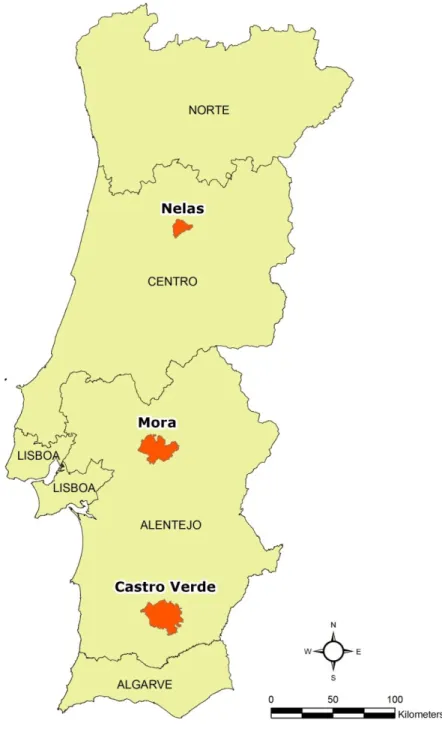
Administrative Cartography) and projections, MMUs and scales will follow the CORINE land cover 2006 defaults (Caetano, Nunes et al. 2009; IGP 2009). For the study of scale effect on carbon stock, portions of the country were chosen across Portugal where different classes could be analyzed. Hence, Nelas, Mora and Castro Verde municipalities were selected for testing (Figure 6).
Portugal is located in the southwest region of Europe on the Iberian Peninsula. Portugal is bordered by the Atlantic Ocean to its west and south and by Spain to its north and east. Makes part of Portugal the Atlantic archipelagos of Azores and Madeira, but these will not be part of this study as it will only describe Continental Portugal.
Continental Portugal is split by its main river, the Tagus. To its North, the landscape is mountainous in the interior with plateaus indented by river valleys. To its South, Portugal features mostly rolling plains and a climate somewhat warmer and drier than in the north. The highest point can be reached in Serra da Estrela, with an altitude of 1,993 m.
Portugal has a Mediterranean climate, Csa in the south and Csb in the north, according to the Köppen climate classification. Portugal is one of the warmest European countries with the annual average temperature in the continent varying from 13 °C to over 18 °C in some areas. Average rainfall varies from more than 3,000 mm in the mountains in the north to less than 600 mm in southern parts of Alentejo.
Portugal has an administrative structure of 308 municipalities, 18 Districts plus two autonomous islands, and 7 regions according to the Nomenclature of Territorial Units for Statistics (NUTS II), being two of them of autonomous administration (Islands of Madeira and Azores).
10
covered by 51% of its area by broad-leaved forests followed by mixed specieis forest (17%) and non irrigated arable land (10%). The landscape is very continuous throughout most of the area. Castro Verde has 68% of its area covered by non irrigated arable land followed by 13% of broad leaved forests. Again, the landscape is not fragmented, showing much continuity especially for the agricultural and forest lands.
11
Figure 6: Location of the three MMU study areas over Continental Portugal, represented by the CAOP 2009 limits with NUTS II division (Adapted from: IGP 2009)
1.7 Overview of Document
12
On part two a literature review on remote sensing and GIS is structured to provide information on the uses of these tools for carbon stock estimation. Further on, examples of specific studies are explained for the reason that they play a major role in the inspiration of this thesis.
13
2. REMOTE SENSING AND GIS AS TOOLS FOR CARBON STOCK
MONITORING
2.1 Remote Sensing
Remote sensing can be briefly defined as the acquisition of information of an object through the use of sensors that are located away from the object, in a way where no contact is possible. In the field of Earth observation and near Earth observation the term remote sensing usually refers to the use of space or airborne imaging sensors who gather and record reflected or emitted energy for users to process, analyze and apply that information (CCRS 2005). The sensors can be divided into two categories, passive and active. The passive sensors receive radiation that are reflected or emitted by an object. In the other hand, active sensors provide the radiation needed to reflect from the objects. In passive sensors, the source of radiation is usually the light provided by the sun while in active sensors the most common form of radiation emitted is RADAR (Radio Detection and Ranging). Passive sensors have the capability of collecting and processing radiation from different parts of the electromagnetic spectrum. What this means is that the sensor can process information from the visible part of the spectrum all the way to Infrared, a very important part where information on vegetation can be analyzed (Campbell 2002).
14
much of the land surface a sensor is capable of registering. And cost refers to the actual economic cost that an operation with a specific sensor may have. Remote sensing can help provide data and focus on measuring GHG sources and sinks by observing land transformation or, in other words, analyzing change detection (Melesse, Weng et al. 2007). It shows to be a perfect tool for environmental monitoring and therefore also for vegetation carbon stock monitoring.
Not only are satellite sensors different in resolution, coverage and cost but there are also different methods and techniques for measuring vegetation carbon stock and sequestration. These differences between them may vary in time labor, techniques, need of special software and especially in investment. Although remote sensing looks promising, some complications are naturally observed. Cloud cover for instance is sometimes presents year-round and impossible to overcome for optical remote sensing. Flooding also imposes difficulties when trying to measure vegetation carbon stock. Selective logging and forest diversity is another crucial discussion when a land classification is considered. The removal of specific species may imply differences in total carbon stored but may not imply on a distinct change in an image pixel value. As for forest diversity, methods for quantifying carbon in a forest with single species is significantly different from a mixed species forest (Vincent, Saatchi 1999).
According to Goetz et al. (2009) there are four approaches to mapping carbon stocks from satellite observations, (i) Synthetic Aperture Radar (SAR), (ii) Light Detection and Ranging (LIDAR), (iii) Optical and (iv) Multi Sensor. All of these rely on calibration of the sensored measurements with estimates from ground-field study sites. The field measurements are usually allometric relations between stem diameter, density and canopy height.
15
placed into categories such as different kinds of forests, grasslands, bare soil and so on. The range of carbon density values is gathered in literature or in field observations for local projects. The LULC classes are multiplied by its respective carbon density to estimate total carbon stock. This approach may be limited by the number of classes and definition of each class but shows an easy and fast way of estimation.
The last approach is defined as Combine & Assign (CA) and is considered as an extension of the last one. The difference is that essentially this approach makes use of further data sets and spatial information to make better estimates. For example, with the help of GIS, data sets with meteorological and soil information may be added to weigh the original carbon density values.
2.2 Land Use /Land Cover
Although they are used sometimes with the same meaning, land cover and land use are actually different from one another. Land cover refers to the surface cover found at a specific location on the ground, being it some vegetation, soil, or urban area. Land use in the other hand refers to the function that the land serves for, being it a recreation area, park, agriculture, and so on.
It is interesting to identify and map land cover for its importance in monitoring studies in a wide field of activities. When a set of land cover maps are available in a time series, it is possible to make temporal analysis. A comparison of land cover maps is referred to as land cover change detection.
LULC change is widely considered as one of the factor concerning the cycle of carbon. It is a notable influence on concentration of CO2 in the atmosphere and particularly on the concentration of other forms of carbon on the biosphere. IPCC estimates that LULC change can contribute up to 1.6 ± 0.8 Gt of carbon per year to the atmosphere in a global perspective. Also, from 1850 to 1998 about 136 ± 55 Gt of carbon have been emitted as a result of LULC change. One major source of this is through the conversion of forests into other land classes (IPCC 2000).
16
account for changes resulting from afforestation and reforestation but voluntary for emissions from forest management, cropland management, grazing, grazing land management and revegetation (UNFCCC 2006).
LULC maps derived from remote sensed images are of great potential for studies such as the one presented in this thesis. The fact that there are several LULC projects and programs around the world and at different levels of coverage make of this tool or data an interesting approach to diverse environmental studies. There are LULC programs that are specific to local actions but there are also programs that are nationwide or even have global coverage. A good example of a well defined and concrete program is the CORINE land cover program from the European Commission. It proves to be of great interest for this study since it embraces the country of Portugal in three distinctive years. More information on the CLC can be found on section 3.1.1.
2.3 Geographic Information Systems
GIS can be defined as a complex system or science that grips large quantity of spatial information. The “geographic” implies that the information is geographically located and therefore is georeferenced. As for the “Information System” it implies that all information is contained in a database that can be accessed by the user for needs such as to analyze, model or edit the spatial phenomena or objects there contained. Goodchild (1988) also remarks that GIS is an “integrated computer system for input, storage, analysis, and output of geographically referenced information”. Its content is a system containing geographically referenced information for the purpose of spatial decision making.
GIS have applications in a variety of professional fields. It can contribute not only to specific fields such as management, science, marketing and logistics but can also link various other fields such as archaeology, environmental impact assessments, agriculture, meteorology urban planning, forestry and so on to its geographical principals. GIS can aid researcher in problem solving when geographic interpretation is needed.
17
Another very important component of GIS is scale. When we represent the real world in piece of paper or on a computerized map, scale is always an important factor for visualization and storage but also a strong tradeoff between the spatial resolution and the amount of information detailed and contained as an attribute (Longley, Goodchild et al. 2005).
2.3.1 Scale
The aspect of scale is known to be central to geography. It states the ratio between a drawn object and the object in real life or a distance on a map and distance in real life. In Goodchild (2001) the author makes a fine review of the meaning of scale, especially in today’s digital world. Terms such as levels of spatial detail, representative fraction, spatial extent and ratios are also reviewed.
Scale provides one of the main characteristics of geographic data which relates to spatial attributes such as form, process, and dimension. The term scale may include different aspects including spatial, temporal and spatio-temporal. The best scale is always dependent on the study objectives, the type of environment and the kind of information desired. Operational scale is described as the spatial extent of the operation of an observable object or phenomena. This is associated, but not equivalent, to the concept of the MMU, which is the smallest size object represented in a map (Lam, Quattrochi 1992).
A MMU can be defined as the “smallest size areal entity to be mapped as a discrete entity” (Lillesand, Kiefer et al. 2003) or as the “smallest polygon which a cartographer is willing to map” (Quattrochi, Goodchild 1997). It is an important figure in studies since it allows reducing the complexity of information on a map when this information is of little or no interest for the purpose of the development of the map. MMU can reduce salt and pepper effect and increase accuracy of remote sensed data.
18
Results indicated that larger MMU significantly affected accuracy estimates of the classification. When using MMU of 6.4 ha, accuracy seemed to be statistically as good as when using MMU of 1.6. The study provides “exceptional information on the flexibility to choose from a range of MMUs that can provide similar accuracy estimates”.
Carrão, Caetano (2002) approached a study with the objectives of evaluating if “metrics that capture landscape pattern are independent of variation in spatial data and if they are sensitive to changes in landscape pattern.” Their study was considered to be of enormous interest since it could show the sensitivity of landscape metrics to scale and in the case of insensitivity, different regions mapped with different resolutions could be compared. Also, remote sensing data at a smaller resolution could be used more often for the production of maps for landscape analysis. Using MapGen (Carrão, Henriques et al. 2001), the COS90 land cover of Portugal was generalized from its original 1 ha MMU to 3, 5, 10, 15, 20 and 25 ha. The landscape metrics analyzed were richness, diversity, dominance, contagion, fractal dimension, large patch index, patch density and edge density. The study results showed that richness, diversity, edge density and large patch index metrics illustrate related performance of covariance at different MMU. The first three had negative covariance meaning that an increase in MMU causes decrease in their values as for the last it is the opposite. The rest of the metrics presented low covariance values which show that the MMU does not explain the changes occurred. Statistical models pointed to a significant effect of MMU over metric values and that their computation for landscapes with different and small MMU could not be compared.
2.4 Vegetation Carbon Stock Studies
Science has come a long way on carbon stock monitoring and modeling. A diverse quantities of studies have been published around the world referring to accounting vegetation carbon stock on specific areas, projects, nations or even globally.
-19
Difference”. Usually, carbon inventory is expressed as metric tons of CO2 emission or removal per hectare per year but it can also be expressed as changes in carbon stocks in metric tons of carbon per hectare over a defined period of time. Also important to define is the difference between net carbon “emission” and “removal”. The first indicates the amount of CO2 or C lost from biomass and soil to the atmosphere by means of decomposition or combustion. The second refers to the opposite where CO2 or C is removed or sequestrated from the atmosphere and stored in biomass and soil.
There are currently several programs that require carbon inventory each one with specific methods and guidelines to follow. It is becoming common to require carbon inventory for projects that result in interventions such as land use change, extraction of biomass, afforestation, deforestation or even soil disturbance. Some of the most known programs that require carbon inventory today either at a project level or national are the National Greenhouse Gas Inventory, Climate Change Mitigation Projects or Programmes, Clean Development Mechanism Projects, Projects Under the Global Environment Facility and Carbon Inventory for Forests, Grassland and Agroforestry Development Projects (UN 1992; IPCC 2006; UNFCCC 2006; GEF 2009).
When referring to approaches to estimate carbon stocks, three methods come to mind, (i) use of default values, (ii) cross-sectional field study and (iii) modeling. Default values are values that have come from different literature reviews, databases or other studies from similar environments. When default values are not ideal or not at all available, researchers have to rely on the generation of their own data through field and laboratory analyses. This method is referred to as cross-sectional field study. Modeling is a method used usually to make projections of future carbon stocks through the use of data acquired through a defined period of time. Therefore, models require both carbon stock estimates and rates of change (Ravindranath, Ostwald 2008).
20
derived from remotely sensed imagery were used together with ground truth data to estimate carbon stock. Strategies to account for carbon stock and change detection using LULC maps and average vegetation carbon density look promising in situations where LULC maps are widely available, especially if an national inventory is the demand.
In Moraes et al. (1998) carbon densities were introduced as attributes to land cover classes. The study was based on a specific area in the Brazilian Amazon in the state of Rondonia. Total carbon stock was calculated using estimates of above ground biomass, soil carbon stocks and changes due to land exploitation.
Land cover maps were produced from Landsat thematic mapper images acquired on July 7th 1991. The classes used were forests, pastures with more than five years, pastures between three and five years of age, pastures with less than three years, rural residential, water, and road.
Values used to estimate carbon stock came from a diverse literature review on local studies. Aboveground carbon density used values of 158 t C ha-1. Burning coefficient was estimated to be 46%. Belowground carbon density was estimated to be 28 t C ha-1. Decay of unburnt biomass was estimated to be 20.9%. Pasture growth per year was estimated to be 6.4 t ha-1 while its combustion efficiency of 94%. Soil carbon was found to lose carbon derived from forest after deforestation and gain carbon after pastures establishment. From zero to three, three to five and five to twenty years after deforestation, the soil would lose 0.5, 0.3 and 0.7 kg cm-2 respectively. After the establishment of a pasture land the soil would gain carbon at a rate of 0.7, 0.4 and 1.2 kg cm-2 between the years zero and three, three and five and five to twenty, respectively. Results showed that carbon stored in untouched forests was of 220 t C ha-1.
21
A special attention is given to Cruickshank et al. (2000), a study on the application of CLC and carbon stock estimation done for the country of Ireland. The main objective was to make in initial inventory of land cover carbon stock for the year of 1990 using a similar strategy to the one to be used in this current study.
The authors used an SM approach where carbon densities for each land cover type were derived from specific studies. Each density was calculated using information found on previous studies related to the land cover class and its national carbon density equivalent. All classes found In Ireland were attributed a value as long as some vegetation was present. Special attention was given to the fact that values of density were only considered for stems, branches, foliage and roots, therefore not including litter, microbial biomass and organic carbon found on the soil. Details on densities and processes undertaken to retrieve values for this study can be found in the Appendix 1 along with Table 7.
Carbon density for each of these land cover classes were multiplied by the area calculated and stored on the feature attribute table. Results showed that Ireland as a whole contains 23.08 Mt of carbon.
The authors pointed out that many improvements could be made towards the estimation of carbon densities for each class. Special attention was given to the improvement of national and local inventories, not having therefore to rely on estimate values from other countries, default values or derived values from other classes.
Not only the density values were noted to be improved but also the basis of this study which is the CORINE land cover. It is stated that the land cover may be underestimating certain classes that could make the total carbon stock even greater. This is the case of forest areas, which on CORINE land cover are only represented if greater than 25 ha.
22 2.5 Conclusions
23
3. MATERIALS AND METHODS
3.1 Materials
Materials used in this study are composed of commercial software such as ArcGIS 9.3, institution developed software such as MapGen (for generalization) and thematic LULC maps from both CORINE and COS land cover projects.
3.1.1 Data
For step one in this study, the thematic LULC maps used are from the CORINE land cover project, which is part of the CORINE program “intended to provide consistent localized geographical information on the land cover for Member States of the European Community” (EC 1992).
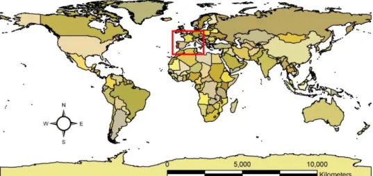
The program was found necessary because it counts as an essential part for the management of the environment and natural resources. At a community level, the CLC is directly useful for determining and implementing environmental policies and can be used combined with other data (e.g. carbon density) to make other complex assessments (e.g. mapping carbon stock) (EC 1992). For the period of 1985 till 1990, the European Commission put into practice the Corine Programme. Throughout this attempt an information system on the state of the environment was created along with methodologies. The CLC was born originally for the 12 participating countries but has now grown to 38, as seen on Figure 7 (EEA 2007).
The CLC maps use a scale of 1:100.000, MMU of 25 hectares and minimum width of linear elements of 100 meters (Table 1). CLC mapping represents a trade-off between production costs and level of detail of land cover information (Heymann, Steenmans et al. 1994).
24
Figure 7: CLC participating countries (Source: EEA 2007)
Table 1: Specifications of each CLC map (Source: EEA 2007)
25
26
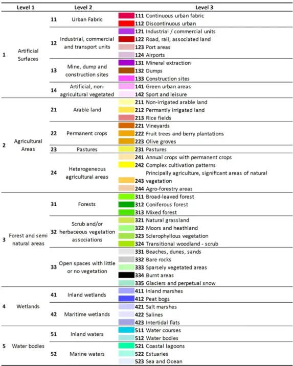
Table 2: CORINE Land Cover nomenclature and legend for all CLC maps in this study (Adapted from: EEA 2007)
27
1990 with the addition of near-infrared composition (Caetano, Pereira et al. 2008).
For comparison reasons the COS90 land cover nomenclature was pre converted into the CORINE land cover nomenclature. The converted vectors were offered by the Portuguese Geography Institute (IGP) as results from a previous project which also offered all generalized shapefiles (Carrão, Caetano 2002). The COS90 land covers, original and already generalized, can be seen on Figure 9, Figure 10 and Figure 11, for Castro Verde, Nelas and Mora, respectively.
Data on vegetation carbon density was provided or adapted from tables found on The Portuguese National Inventory Report on Greenhouse Gases, 1990-2007 (and on the 1990-2004) Submitted under the United Nations Framework Convention on Climate Change and the Kyoto Protocol (Ferreira, Pereira et al. 2006; Pereira, Seabra et al. 2009). For some missing values, the study made in Ireland was chosen as the best source for adapting values (Cruickshank, Tomlinson et al. 2000). Values were noted to be respecting the IPCC Good Practice Guidance for Land Use, Land Use Change and Forestry (IPCC 2003). Also is important to mention that these values of carbon density take into account stems, branches, foliage and roots but do not include litter, microbial biomass and organic carbon found on the soil. In Table 8 of the Appendix 2, a set of information on the description of choice for the carbon density values are presented.
28
Figure 9: COS90 land cover maps of Castro Verde containing the original 1 ha MMU along
with all generalizations up to 25 ha – all reclassified into CLC nomenclature (Adapted
29
Figure 10: COS90 land cover maps of Nelas containing the original 1 ha MMU along with
all generalizations up to 25 ha – all reclassified into CLC nomenclature (Adapted from:
30
Figure 11: COS90 land cover maps of Mora containing the original 1 ha MMU along with
all generalizations up to 25 ha – all reclassified into CLC nomenclature (Adapted from:
Carrão, Caetano 2002)
3.1.2 Software
31 3.2 Methods
3.2.1 Carbon Stock Estimation Using CORINE Land Cover
In this study, the CLC90 (1985), CLC00 (2000) and CLC06 (2006) thematic maps in vector form provided the basis for the estimation of vegetation carbon stock in Continental Portugal for each of the described years. Each dataset accounts land cover information on location, area and class for each of the respective years studied (Caetano, Nunes et al. 2009). A SM approach was used along with carbon density information (Ferreira, Pereira et al. 2006; Pereira, Seabra et al. 2009) and the auxiliary shapefiles (IGP 2009).
32
Level 3 CLC Nomenclature
Area (ha) Carbon Density (t ha-1)
CLC90 CLC00 CLC06
111 Continuous urban fabric 10434 12105 12260 0.00
112 Discontinuous urban 162013 202438 215336 4.71
121 Industrial / commercial units 16727 29920 33912 0.00
122 Road, rail, associated land 568 2256 7679 0.00
123 Port areas 1685 1942 2087 0.00
124 Airports 3861 4216 4303 0.50
131 Mineral extraction 6108 12249 13662 0.00
132 Dumps 333 748 972 0.00
133 Construction sites 3061 5735 6520 0.00
141 Green urban areas 1596 1774 1774 9.42
142 Sport and leisure 5324 9098 11536 9.42
211 Non-irrigated arable land 1091750 1019420 981762 5.00
212 Permantly irrigated land 137244 203811 210529 5.00
213 Rice fields 55245 54401 52825 5.00
221 Vineyards 196575 222741 228989 21.00
222 Fruit trees and berry plantations 95493 100566 100994 21.00
223 Olive groves 271093 262925 263050 21.00
231 Pastures 54414 42104 41875 6.00
241 Annual crops with permanent crops 433479 405798 404030 13.00
242 Complex cultivation patterns 624563 609919 607114 11.52
243 Principally agriculture, significant areas of
natural vegetation
736818 700130 686894 11.37
244 Agro-forestry areas 634862 628700 621494 8.22
311 Broad-leaved forest 1059381 1125182 1007057 28.24
312 Coniferous forest 786646 708637 534028 59.48
313 Mixed forest 561518 545361 475573 40.80
321 Natural grassland 185652 176184 171911 6.00
322 Moors and heathland 314570 289488 284612 17.74
323 Sclerophyllous vegetation 264975 225165 206788 17.74
324 Transitional woodland - scrub 896696 1019236 1411524 17.74
331 Beaches, dunes, sands 11865 11831 11830 0.00
332 Bare rocks 23768 23854 23881 0.00
333 Sparsely vegetated areas 99016 100528 100835 3.00
334 Burnt areas 46274 29688 32862 0.00
335 Glaciers and perpetual snow
411 Inland marshes 1048 1119 1139 1.50
412 Peat bogs
421 Salt marshes 18712 18509 18459 2.00
422 Salines 7117 7229 7229 0.00
423 Intertidal flats 1775 1775 1993 0.00
511 Water courses 20753 20595 19876 0.00
512 Water bodies 28855 34600 52989 0.00
521 Coastal lagoons 8475 8523 8547 0.00
522 Estuaries 45284 45113 44919 0.00
523 Sea and Ocean 2411448 2411464 2411428 0.00
Table 3: CORINE land cover third level nomenclature and respective area sizes with applied carbon density values (Adapted from: Cruickshank, Tomlinson et al. 2000;
Caetano, Nunes et al. 2009; Pereira, Seabra et al. 2009)
33
vector resulting in an exact perimeter for each file, renamed to CLCXX_CAOP, being “XX” the original CLC map. The density table, previously made, was joined with the attribute table of the CLCXX_CAOP so that density values would appear on the vector attributes. Geometry was calculated to find out each polygons exact area in hectares. Now, with the vector file containing density values (t ha -1) and area (ha), a simple multiplication was made on the attribute table resulting in another column with the vegetation carbon stock for that specific feature (in metric tons). Statistical analysis and summaries were made with these resulting values.
A second step in the GIS procedures was accomplished to reveal the vegetation carbon stock spatial distribution. For visualization and calculation purposes, it was decided that the best method was to convert each CLCXX_CAOP map into a grid system of 2500 ha. For this, the Hawths Analysis Tools in ArcGIS environment was applied to create a grid system called CLC_GRID with specific ID for each cell. The CLCXX_CAOP and the CLC_GRID were united using the UNION function of ArcGIS, resulting in a file called CLCXX_CAOP_UNION. This file was later dissolved by the ID of each cell on the grid system with the function of summing the carbon stock attribute of each cell. This procedure resulted in the vegetation carbon stock spatial distribution map for each CLC year map, organized in cells of 2500 ha and named CLCXX_CAOP_DISSOLVE. A final GIS procedure was undertaken to analyze vegetation carbon stock change detection. In this step each of the dissolved maps was intersected resulting in a final shapefile named CLC_CSCHANGE which contained information on vegetation carbon stock for each study year and each cell. After a field calculator procedure, three new columns were created representing the change over three periods, from 1985 to 2000 (00-85), from 2000 to 2006 (06-00) and from 1985 to 2006 (06-85). This procedure resulted in three maps representing the vegetation carbon stock change detection.
34
Figure 12: Flowchart of the GIS procedures undertaken
35
ID CLC Level 3 Nomenclature Mega Class
111 Continuous urban fabric Artificial Area
112 Discontinuous urban Artificial Area
121 Industrial / commercial units Artificial Area
122 Road, rail, associated land Artificial Area
123 Port areas Artificial Area
124 Airports Artificial Area
131 Mineral extraction Artificial Area
132 Dumps Artificial Area
133 Construction sites Artificial Area
141 Green urban areas Artificial Area
142 Sport and leisure Artificial Area
211 Non-irrigated arable land Agriculture
212 Permantly irrigated land Agriculture
213 Rice fields Agriculture
221 Vineyards Agriculture
222 Fruit trees and berry plantations Agriculture
223 Olive groves Agriculture
231 Pastures Agriculture
241 Annual crops with permanent crops Agriculture
242 Complex cultivation patterns Agriculture
243 Principally agriculture, significant areas of natural
vegetation
Agriculture with Natural Area
244 Agro-forestry areas Agriculture with Natural Area
311 Broad-leaved forest Forest
312 Coniferous forest Forest
313 Mixed forest Forest
321 Natural grassland Natural Area
322 Moors and heathland Natural Area
323 Sclerophyllous vegetation Natural Area
324 Transitional woodland - scrub Forest
331 Beaches, dunes, sands Natural Area
332 Bare rocks Natural Area
333 Sparsely vegetated areas Natural Area
334 Burnt areas Natural Area
335 Glaciers and perpetual snow Natural Area
411 Inland marshes Natural Area
412 Peat bogs Natural Area
421 Salt marshes Natural Area
422 Salines Natural Area
423 Intertidal flats Natural Area
511 Water courses Water
512 Water bodies Water
521 Coastal lagoons Water
522 Estuaries Water
523 Sea and Ocean Water
Table 4: Adapted Mega Class nomenclature from the CLC third level nomenclature
3.2.2 The Effect of Scale (MMU) On Carbon Stock Estimation
36
The COS90 maps for each city were previously generalized from its original MMU of 1 ha into 3, 5, 10, 15, 20 and 25 ha maps. In all, twenty one different maps were made available, seven for each city. The comparison of each map was expected to deliver information on the effects of scale on carbon stock estimation. Generalization was made by MapGen software (Carrão, Henriques et al. 2001). The MapGen application runs on ArcView 3.2 and allows non-expert users to automatically generalize COS90 maps to the CORINE land cover classification scheme using the desired MMU values. The set of rules for the generalization procedures were based on the CORINE land cover technical guide specifications for manual generalization (Heymann, Steenmans et al. 1994). All this previous work was a result from studies undertaken by the IGP Remote Sensing Group (Carrão, Caetano 2002), who also donated this dataset.
The first steps in this study were similar to the previous study. Data was first prepared for analysis which meant converting spatial information into the reference system to be used throughout the study. For this, the projected coordinate system established was the ETRS_1989_Portugal_TM06, same used on the original CLC06 data. Projection was established as Transverse Mercator with units in Meters. Carbon density values used are exactly the same used on the first study.
37
Figure 13: Flowchart of the GIS procedures undertaken
3.3 Summary
38
4. RESULTS AND DISCUSSION
4.1 Vegetation Carbon Stock Estimation Using CORINE Land Cover
After pre-processing and preparing all spatial data for the current study projections, the CLC maps were clipped to the CAOP 2009 official administrative division. These maps guaranteed a symmetrical comparison in between maps and also guaranteed official divisions and borders for the study outputs.
The first step in the GIS procedures resulted in land cover maps of vegetation carbon stock. From these maps it was possible to retrieve information on a final summary of vegetation carbon stock in Portugal for the years 1985, 2000 and 2006. Values showed a high decrease of carbon over the years, especially from 2000 to 2006. The year 1985, derived from the CLC90, turned out with a total of 173.08 Mt of carbon. The years 2000 and 2006 resulted in 170.22 Mt and 159.97 Mt of carbon, respectively.
39
Figure 14: Vegetation carbon density values applied for each CLC class (Adapted from: Cruickshank, Tomlinson et al. 2000; Pereira, Seabra et al. 2009)
Figure 15: Vegetation carbon stock is represented for each CLC class with carbon density
values ≠ 0
0 10 20 30 40 50 60 70 Ve ge ta tion C a rbon D e n s it ie s in t h a -1 CLC Classes
Vegetation Carbon Density for CLC Classes
0 5 10 15 20 25 30 35 40 45 50 Ve ge ta tion C a rbon S toc k in M t CLC Classes
Vegetation Carbon Stock for Each CLC Class
1985
2000
40
Figure 16: Corresponding area size for each CLC class with carbon density values ≠ 0
On the last two graphs, the most visible changes that have occurred over the years are noted on the classes of Coniferous Forests (312), Mixed Forests (313) and Transitional Woodlands – Scrub (324). The first has had a high decrease in both area and in carbon stock, resulting in a 32.1% change. Mixed Forests has also had a high decrease in both area and carbon stock with changes of 15.3%. In the other hand, Transitional Woodlands – Scrubs had a higher change with an increase 57.4% in both area and carbon stock.
The carbon density graph works as an auxiliary tool for interpretation of the other two distribution graphs presented. By comparing and analyzing these three sources of information it is possible to suggest that classes 312, 313 and 324 have an intimate relation to one another. These classes represent the highest values in carbon density with values of 59.48, 40.8 and 17.74 t ha-1, respectively. If we take into account that the first two classes correspond to the highest concentrations of carbon stock it is also possible to say that any decrease in their area should reflect in a high decrease in total vegetation carbon stock. Following this theory, it is also possible to suggest that a decrease in forest areas may lead to an increase in transitional woodland areas.
According to the European Environmental Agency (EEA 1997), the short definition for the class 324 refers to a bushy or herbaceous vegetation with scattered trees which can represent either woodland degradation or forest
0 2 4 6 8 10 12 14 16 Ar e a ( h a ) x 1 0 0 0 0 0 CLC Classes
Area Size for Each CLC Class
1985
2000
41
regeneration/colonization but may also refer to new plantations or even recently cut plantations. If we take this into account than it is possible to state that the deforestation of classes 312 and 313 may lead to class 324. Proof of a supposition such as this one is plausible if we consider the series of forest fires that Portugal has been hit with the last few years. A forest fire could be a reasonable source for the phenomena shown by the presented graphs.
In an effort to better interpret and visualize the information gathered, a set of “mega classes” were derived from the CLC nomenclature. A table with resulting information is presented in Table 10 of the Appendix 2. Two graphical representations may be viewed in Figure 17 and Figure 18 where distribution of area size and carbon stock is represented, respectively.
Figure 17: Distribution of area of each Mega Class per year 0
50 100 150 200 250 300 350 400
1985 2000 2006
Ar
e
a
(
h
a
)
x
1
0
0
0
0
Year
Mega Classes Area Size per Year
Artificial Areas
Agriculture
Agriculture with Natural Areas
Forests
Natural Areas
42
Figure 18: Distribution of vegetation carbon stock of each Mega Class per year
Results showed and confirmed the superior concentration of carbon stock on forest related classes. Numbers established a concentration of carbon stock in between 65% and 67% on forest lands with the second largest concentration in agricultural lands with values between 18% and 20%. As far as changes in carbon stock, forests also had the highest change with total loss of 10.88 Mt, followed by natural areas with 1.64 Mt. By examining the two distribution graphs it is clear to see the increase in forest area and decrease in forest carbon stock. Again, this phenomenon may be explained by the fact that high carbon density forests have been lost (classes 311, 312 and 313) while low carbon density forests have been gained (class 324). Using the same example from before, forests such as broad-leaved, coniferous or mixed could have been somehow deforested making space for low density forests such as transitional woodlands, degraded areas, regeneration land and so on.
To account for a spatial distribution of carbon throughout the country, a grid system of 2500 ha was developed. This step was crucial for better visualization of the spatial distribution and also to permit and facilitate a change detection strategy. Spatial distribution maps of 1985, 2000 and 2006 are represented in Figure 19, while change detection maps for the period of 1985-2000, 2000-2006 and 1985-2006 are represented in Figure 20.
0 20 40 60 80 100 120 140
1985 2000 2006
Ve ge ta tion C a rbon S toc k ( M t) Year
Mega Classes Vegetation Carbon Stock per Year
Artificial Areas
Agriculture
Agriculture with Natural Areas
Forests
Natural Areas
43
44
45
For identification reasons and to facilitate interpretation of the spatial distribution of carbon stock, the information was also presented with the NUTS II official administrative division. A series of information on distribution of area and carbon stock can be seen on Table 5 and in Figure 21.
1985 2000 2006 NUTS II Area
(ha) Area (%) C Stock (Mt) Density (t/ha) C Stock (Mt) Density (t/ha) C Stock (Mt) Density (t/ha)
ALENTEJO 3155119 35.5 48.51 15.4 49.07 15.6 48.2 15.3
ALGARVE 499597 5.6 8.27 16.6 8.36 16.7 8.15 16.3
CENTRO 2820009 89.4 71.57 25.4 69.36 24.6 62.58 22.2
LISBOA 294011 3.3 4.57 15.5 4.08 13.9 4.05 13.8
NORTE 2128392 23.9 40.16 18.9 39.35 18.5 36.98 17.4
Table 5: Distribution of area and vegetation carbon stock over the NUTS II administrative division for the three years studied
Figure 21: Distribution of vegetation carbon stock for each NUTS II administrative division over each of the three years studied
The spatial distribution maps show a clear distribution of carbon throughout Continental Portugal with focus on the high concentration of carbon stock in the Centro region of the country, followed by the Norte region, according to Table 5. This high concentration of carbon stock in Centro region can be an influence of the presence of different types of forest lands according to the original CLC maps. The same maps give an overview of lower concentration of carbon in the Alentejo and Lisboa regions.
As for the change detection maps, a high loss of carbon stock is verified especially in the Centro region as can be proven by values found on Table 5. In
0 10 20 30 40 50 60 70 80
ALENTEJO ALGARVE CENTRO LISBOA NORTE
Ve ge ta tion C a rbon S toc k ( M t)
NUTS II Administrative Division
Distribution of Carbon Stock For Each NUTS II Administrative Division Over Three Years
1985
2000
46
all, the Algarve and Alentejo regions suffered the least change, both in increase and decrease. It is possible to state that the regions that most lost carbon are exactly the forest regions of the central and northern part of Portugal.
4.2 The Effect of Scale (MMU) On Vegetation Carbon Stock Estimation
A final summary of carbon stock for the cities of Castro Verde, Nelas and Mora for the year 1990 (COS90) at different MMUs can be seen on Table 6. Values tended not to vary much as MMU were changed, having Castro Verde a small decline, Nelas a small increase and Mora fluctuated up and down with no correlation at all (Figure 22).
Minimum Mapping Units
Study Area 1 ha 3 ha 5 ha 10 ha 15 ha 20 ha 25 ha CLC90 25 ha C a rb o n St o ck (t * 1 0 0 0
) Castro Verde 509 507 505 502 500 500 497 419
Nelas 342 347 347 344 342 350 348 425
Mora 1116 1119 1122 1130 1136 1142 1143 674
Table 6: Vegetation carbon stock for each MMU
Figure 22: Distribution of carbon stock throughout different MMUs with addition of a linear trendline
Full information tables containing values per class were also created for each study site and are presented in the Appendix 3 on Table 11 for Castro Verde, Table 12 for Nelas and Table 13 for Mora.
y = -1.9848x + 510.91 R² = 0.9634
y = 0.7341x + 342.88 R² = 0.2435 y = 5.0451x + 1109.7
R² = 0.9785
0 200 400 600 800 1000 1200 1400
1 ha 3 ha 5 ha 10 ha 15 ha 20 ha 25 ha
Ve ge ta tion C a rbon S toc k ( t * 1 0 0 0 )
Minimum Mapping Units
Distribution of Carbon Stock Throughout Different MMUs
Castro Verde
Nelas
Mora
47
For better visual analysis, six separate graphs were produced; one for each municipality, showing the distribution of the vegetation carbon stock and LULC area size for each one of the MMUs over the CLC adapted nomenclature. Castro Verde is presented in Figure 23 and Figure 24, Nelas in Figure 25 and Figure 26 and Mora in Figure 27 and Figure 28.
Figure 23: Vegetation carbon stock for each MMU of Castro Verde study area
Figure 24: Area size for each MMU of Castro Verde study site 0 50 100 150 200 250 Ve ge ta tion C a rbon S toc k ( t) T h ou s a n d s
Nomenclature Adapted From The CLC
Vegetation Carbon Stock for Each MMU of Castro Verde 1 ha 3 ha 5 ha 10 ha 15 ha 20 ha 25 ha 0 5 10 15 20 25 30 35 40 45 Ar e a ( h a ) T h ou s a n d s
Nomenclature Adapted From The CLC
Area Size for Each MMU of Castro Verde
48
Figure 25: Vegetation carbon stock for each MMU of Nelas study site
Figure 26: Area size for each MMU of Nelas study site 0 20 40 60 80 100 120 140 160 180 200 Ve ge ta tion C a rbon S toc k ( t) T h ou s a n d s
Nomenclature Adapted From The CLC
Vegetation Carbon Stock for Each MMU of Nelas
1 ha 3 ha 5 ha 10 ha 15 ha 20 ha 25 ha 0 1 1 2 2 3 3 4 Ar e a ( h a
) Th
ou s a n d s
Nomenclature Adapted From The CLC
Area Size for Each MMU of Nelas
49
Figure 27: Vegetation carbon stock for each MMU of Mora study site
Figure 28: Area size for each MMU of Mora study site
The city of Castro Verde presented a high concentration of vegetation carbon stock in Broad Leaved Forests (311) and in Non-Irrigated Arable land (211). Both of these had an increase in carbon stock when MMU was increased. The class Coniferous Forest (312) also presented an increase in carbon stock although it is almost insignificant compared to the other two presented. All other classes have decreased carbon stock, some of them even vanishing.
0 100 200 300 400 500 600 700 Ve ge ta tion C a rbon S toc k ( t) T h ou s a n d s
Nomenclature Adapted From The CLC
Vegetation Carbon Stock for Each MMU of Mora
1 ha 3 ha 5 ha 10 ha 15 ha 20 ha 25 ha 0 5 10 15 20 25 Ar e a ( h a ) T h ou s a n d s
Nomenclature Adapted From The CLC
Area Size for Each MMU of Mora