www.earth-syst-dynam.net/5/177/2014/ doi:10.5194/esd-5-177-2014
© Author(s) 2014. CC Attribution 3.0 License.
Earth System
Dynamics
Terminology as a key uncertainty in net land use and land cover
change carbon flux estimates
J. Pongratz1, C. H. Reick1, R. A. Houghton2, and J. I. House3
1Max Planck Institute for Meteorology, Hamburg, Germany 2Woods Hole Research Center, Falmouth, MA, USA
3Cabot Institute & Department of Geography, University of Bristol, Bristol, UK Correspondence to:J. Pongratz ([email protected])
Received: 22 July 2013 – Published in Earth Syst. Dynam. Discuss.: 7 August 2013 Revised: 30 January 2014 – Accepted: 11 February 2014 – Published: 27 March 2014
Abstract.Reasons for the large uncertainty in land use and land cover change (LULCC) emissions go beyond recog-nized issues related to the available data on land cover change and the fact that model simulations rely on a simplified and incomplete description of the complexity of biological and LULCC processes. The large range across published LULCC emission estimates is also fundamentally driven by the fact that the net LULCC flux is defined and calculated in differ-ent ways across models. We introduce a conceptual frame-work that allows us to compare the different types of models and simulation setups used to derive land use fluxes. We find that published studies are based on at least nine different def-initions of the net LULCC flux. Many multi-model synthe-ses lack a clear agreement on definition. Our analysis reveals three key processes that are accounted for in different ways: the land use feedback, the loss of additional sink capacity, and legacy (regrowth and decomposition) fluxes. We show that these terminological differences, alone, explain differ-ences between published net LULCC flux estimates that are of the same order as the published estimates themselves. This has consequences for quantifications of the residual terres-trial sink: the spread in estimates caused by terminological differences is conveyed to those of the residual sink. Fur-thermore, the application of inconsistent definitions of net LULCC flux and residual sink has led to double-counting of fluxes in the past. While the decision to use a specific def-inition of the net LULCC flux will depend on the scientific application and potential political considerations, our analy-sis shows that the uncertainty of the net LULCC flux can be substantially reduced when the existing terminological con-fusion is resolved.
1 Introduction
Future climate change and the required strength of our mit-igation efforts depend strongly on the terrestrial emissions and sinks. The change in the atmospheric carbon content (Catmos) due to anthropogenic activity is determined by the emissions from fossil-fuel burning (Ffossil) and the net ex-change fluxes between atmosphere and ocean (Focean-atmos) and between atmosphere and land (Fland-atmos). Currently, the terrestrial biosphere is a net sink for carbon with 1.4 GtC yr−1uptake over the 2000s (Le Quéré et al., 2013a). This flux Fland-atmos – also called the “net biosphere flux”, “net land flux”, or “net land–atmosphere flux” – is the re-sult of two opposing fluxes, the “net land use and land cover change flux” (FLULCC) and the “residual terrestrial flux” (Fresidual). The global carbon budget can thus be formulated as
dCatmos
dt =Ffossil−Focean-atmos −Fland-atmos
=Ffossil−Focean-atmos +FLULCC−Fresidual, (1) where fluxes Ffossil and FLULCC are defined as positive into the atmosphere, and fluxesFocean-atmos,Fland-atmos, and
Fresidualas positive out of the atmosphere.
use flux” or “net LULCC flux”. The term “net” is added be-cause LULCC be-causes not just emissions to the atmosphere (e.g. when a forest is cleared, or harvested wood products are burnt or decay), but also uptake of CO2from the atmosphere (e.g. from growth of planted or recovering vegetation follow-ing anthropogenic disturbance). The net LULCC flux is of the order of 1.0±0.5 GtC yr−1(Le Quéré et al., 2013a), with a range across 13 different model results (each with specific definitions explained later) compiled in the meta-analysis of Houghton et al. (2012) of 0.8 to 1.5 PgC yr−1for the 1990s.
The difference between the net biosphere flux and net LULCC flux implies a sink, typically known as the “resid-ual terrestrial flux” (Fresidual in Eq. 1) as it is calculated as the residual of other more directly estimated terms in the car-bon budget (i.e. fossil-fuel and LULCC emissions minus at-mospheric growth and ocean uptake). This sink amounts to 2.4±0.8 GtC yr−1 uptake over the 2000s (Le Quéré et al., 2013a) and is corroborated by inventories in intact forests (e.g. Pan et al., 2011). It is thought to be primarily due to the indirect effects of anthropogenic environmental change on terrestrial ecosystems: the fertilizing effects of rising CO2 in the atmosphere, changes in nutrient cycles, and climate change impacts (Zaehle et al., 2011; Le Quéré et al., 2013a; Piao et al., 2013). The indirect effects of environmental change affect both managed and unmanaged (pristine) land. As will be shown in this article, the indirect effects are ac-counted for to very different extents and in very different ways in published estimates of the net LULCC flux. This is partly due to the political or scientific purpose for which a methodology is employed, but is often also constrained by the nature of available data or modelling tools.
The net LULCC flux is the most uncertain of the directly estimated terms in the global carbon budget, and this un-certainty propagates into estimating the residual flux. Since the net LULCC flux is not directly observable on the global scale, models are an essential tool to estimate it. However, model differences induce a major uncertainty in net LULCC flux estimates: of the 13 studies on LULCC emissions in Houghton et al. (2012), and five in Le Quéré et al. (2013a), the underlying model estimates differed particularly with re-spect to the assumed rates of deforestation (partly but not entirely dependent on driving data), the carbon densities for vegetation cleared, and the inclusiveness of management ac-tivities. Some of these uncertainties may be reduced in the future due to increasing data availability: for example, esti-mates of biomass can be derived from observations, which recently have become available on a spatially explicit basis for large regions of the world (Baccini et al., 2012); however, they are still subject to considerable uncertainty and will not be available for the pre-satellite era. In addition, process-based models simulate vegetation biomass as a prognostic variable and as such depend on simplification and parame-terization of various processes. Differences due to input data and processes included in models have been described and
sometimes quantified and account for about 50 % uncertainty in LULCC estimates (Houghton et al., 2012).
However, published estimates contain another source of uncertainty: terminological differences that result from dif-ferences in definition of which flux component to include in the net LULCC flux. These differences result from ad hoc choices in the simulation setup, but are partly predetermined by the type of model used.
Estimates stem from three generations of models, which each simulate the CO2exchange between biosphere and at-mosphere in different ways:
a. Bookkeeping models track changes in the carbon stocks of the areas undergoing LULCC using growth and decay curves of soil and vegetation carbon of predefined shape. In the original bookkeeping ap-proach (e.g. Houghton et al., 1983) carbon densities are based on inventories and do not respond to tran-sient changes in CO2 and climate. Later approaches (e.g. Gitz and Ciais, 2003) include a modification fac-tor to the growth curves depending on the atmospheric CO2concentration to account in a simplified form for the effects of environmental changes on carbon stocks. b. Dynamic global vegetation models (DGVMs) simulate soil and plant processes, and their response to external CO2and climate drivers. These environmental condi-tions are prescribed from data externally and the sim-ulations are thus uncoupled. This means that environ-mental conditions are not altered by the biospheric ac-tivity within the model setup.
c. Earth system models (ESMs) link process-based veg-etation models such as DGVMs interactively with carbon cycle and climate modelling and account for climate- and CO2-mediated feedbacks that could not be represented in uncoupled DGVM simulations: for example, land use change emits CO2and causes bio-geophysical changes in albedo and latent heat flux; these biogeochemical and biogeophysical changes af-fect climate and CO2 concentrations, which in turn feed back on growth and decomposition rates; this in turn affects the net LULCC flux, closing the feedback loop.
Independent of the type of model used, the net LULCC flux is determined with respect to a reference state that ex-cludes changes in land use or land cover; i.e. the net LULCC fluxFLULCCis defined as difference
in a separate simulation; in particular in cases where envi-ronmental conditions are assumed to not change over the course of the LULCC simulation the initial state of carbon stocks and fluxes in the LULCC simulation may serve as an implicit reference. It is also possible to quantify individual flux components, such as instantaneous LULCC emissions, without an explicit reference. However, the without-LULCC reference is crucially needed, implicitly or explicitly, to an-swer the question of LULCC impact as compared to a world that had not seen such human disturbance. Yet the assumed reference state differs between studies, including the vege-tation cover, carbon density and environmental drivers. We will show below how different estimates for the net LULCC flux differ by the assumed reference8noLULCC.
To compare the terminology across published net LULCC flux estimates, we introduce a conceptual framework suitable for distinguishing the different methods. Others (Strassmann et al., 2008; Gasser and Ciais, 2013) have also devel-oped conceptual frameworks to derive flux components for LULCC-induced carbon fluxes, but focus on selected con-cepts and consider only a subset of relevant flux components. By contrast, our study aims to give a comprehensive com-parison of the various methods used in published estimates. While these previous studies provided mathematical formu-lations that allow for actual quantifications of various fluxes, our study aims at a comprehensive, illustrative framework that allows the reader to understand how published estimates of the net LULCC flux differ in terms of their definition due to the specific type of model and model setup used to derive them.
Terminological differences have increased the uncertainty range across estimates of the net LULCC flux unnecessar-ily, because they can be resolved more easily than intrinsic uncertainties in data availability, process understanding, and model parameterizations. More and more climate models as well as economic and trade models have been extended to include LULCC over the past years, and new approaches of quantifying carbon stocks and fluxes directly using data on LULCC and biomass from remote sensing are being devel-oped (Baccini et al., 2012; Harris et al., 2012). To be able to consistently compare past and forthcoming estimates of the net LULCC flux, confusion about terminological issues should be resolved.
2 Materials and methods
2.1 Framework for partitioning the net LULCC flux
The aim of our framework is to break down the various pub-lished estimates of the net LULCC flux into the same flux components. This allows for a direct comparison of which flux components are included and excluded by the various published estimates. Our framework for comparison distin-guishes between land carbon fluxes induced by the direct
effects of anthropogenic LULCC activity (“direct” referring to LULCC-induced changes in vegetation distribution); car-bon fluxes induced by the effects of human-induced envi-ronmental changes, which are anindirectresult of LULCC or other anthropogenic activity; and fluxes that arise due to the combination of direct LULCC effects and indirect effects mediated by environmental changes.
Carbon fluxes from direct LULCC effects involve different timescales. Methodological approaches typically distinguish between “instantaneous emissions” to the atmosphere upon a human intervention like land-clearing fires (termed “I”; see Table 1 for list of abbreviations), and “legacy fluxes” (“L”) from the readjustment of the carbon stocks to the new type of vegetation and/or type and intensity of manage-ment over time. Legacy fluxes include respiration of plant residues (e.g. harvest slash, dead roots) and disturbed soil organic matter, changes in the stocks of products such as pa-per and timber, and recovery of the living carbon stocks. The legacy flux thus comprises sources and sinks. In sustainably managed forests with a harvest regrowth cycle, these gross sources and sinks may be large, but they are of the same or-der of magnitude over time and thus result in a small net flux (Pan et al., 2011; Houghton et al., 2012). The distinction between instantaneous emissions and legacy flux differs be-tween methods to some extent: instantaneous emissions may refer to emissions at the instance of LULCC (e.g. Pongratz et al., 2009b) or all emissions within a year (Houghton et al., 2012). Many of the methods discussed below quantify both fluxes together. However, it is necessary to keep the two fluxes separate in our framework; it will illustrate that the in-stantaneous emissions are the only flux always accounted for, while the legacy emissions are partly omitted by some model approaches. Note that for satellite and some inventory-data-based approaches, the time period of analysis is shorter than the timescale of legacy effects, so that legacy emissions may be partially omitted, or all emissions may be assumed to be instantaneous (e.g. DeFries et al., 2002; Harris et al., 2012; IPCC, 2006; FAO, 2013).
Underlying all processes involved in the legacy flux is a disequilibrium between carbon uptake and loss. For an ecosystem, this disequilibrium is caused by a mismatch of net primary productivity (NPP) and heterotrophic respiration (Rh). Calling NEP = NPP−Rh net ecosystem productivity, NEP6=0 is the signature of disequilibrium. The direct effects of LULCC cause a disequilibrium between NPP andRhthat often lasts decades to centuries, but without further distur-bance systems tend to recover from this imbalance. An equi-librium may also be reached in managed systems if on aver-age the amount of carbon that is extracted from the ecosys-tem is balanced by regrowth, as for example in sustainable forestry.
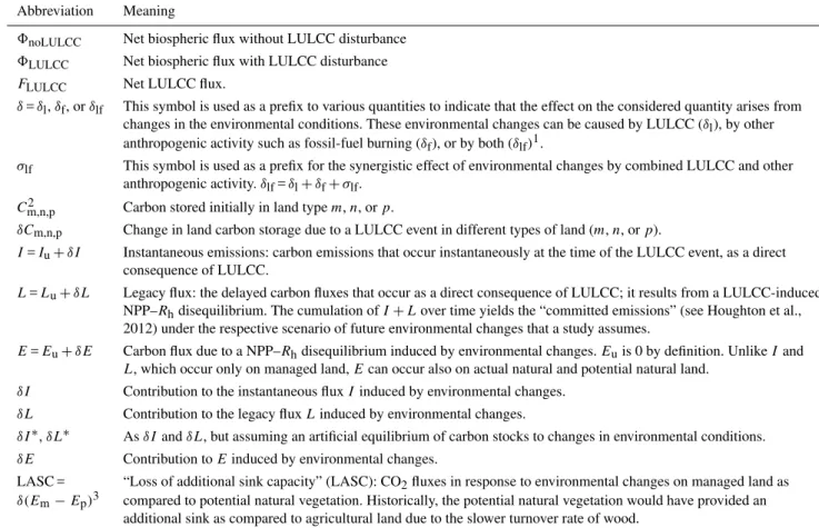
Table 1.Carbon stocks and fluxes used in our conceptual framework for comparison of published studies. See Table 2 for meaning of subscripts.
Abbreviation Meaning
8noLULCC Net biospheric flux without LULCC disturbance
8LULCC Net biospheric flux with LULCC disturbance
FLULCC Net LULCC flux.
δ=δl,δf, orδlf This symbol is used as a prefix to various quantities to indicate that the effect on the considered quantity arises from
changes in the environmental conditions. These environmental changes can be caused by LULCC (δl), by other
anthropogenic activity such as fossil-fuel burning (δf), or by both (δlf)1.
σlf This symbol is used as a prefix for the synergistic effect of environmental changes by combined LULCC and other
anthropogenic activity.δlf=δl+δf+σlf.
Cm,n,p2 Carbon stored initially in land typem,n, orp.
δCm,n,p Change in land carbon storage due to a LULCC event in different types of land (m,n, orp).
I=Iu+δI Instantaneous emissions: carbon emissions that occur instantaneously at the time of the LULCC event, as a direct
consequence of LULCC.
L=Lu+δL Legacy flux: the delayed carbon fluxes that occur as a direct consequence of LULCC; it results from a LULCC-induced
NPP–Rhdisequilibrium. The cumulation ofI+Lover time yields the “committed emissions” (see Houghton et al.,
2012) under the respective scenario of future environmental changes that a study assumes.
E=Eu+δE Carbon flux due to a NPP–Rhdisequilibrium induced by environmental changes.Euis 0 by definition. UnlikeIand
L, which occur only on managed land,Ecan occur also on actual natural and potential natural land.
δI Contribution to the instantaneous fluxIinduced by environmental changes.
δL Contribution to the legacy fluxLinduced by environmental changes.
δI∗,δL∗ AsδIandδL, but assuming an artificial equilibrium of carbon stocks to changes in environmental conditions.
δE Contribution toEinduced by environmental changes.
LASC = “Loss of additional sink capacity” (LASC): CO2fluxes in response to environmental changes on managed land as
δ(Em−Ep)3 compared to potential natural vegetation. Historically, the potential natural vegetation would have provided an
additional sink as compared to agricultural land due to the slower turnover rate of wood.
1We use “δ” without subscript as a general term to refer to any fluxes due to environmental changes, be they induced by LULCC (“l”), by other external drivers such as fossil-fuel
burning (“f”), or a combination of both (“lf”).2Note that for a sum of fluxes or stocks on different areas, such as “Em+En” we sometimes use the shorthand “Emn”.3Note that
for effects of the same environmental changes on different fluxes we write e.g.δ(Em−Ep)as shorthand forδEm−δEp.
different ways and on different timescales to environmental changes. Both NPP andRhare influenced by environmental conditions, for example CO2fertilization effects on NPP and dependence of soil respiration on temperature and moisture. Further,Rhalso depends on NPP. Due to the slow turnover rates of many carbon stocks,Rhfollows the evolution of NPP with a time lag. For example, an increase in NPP initially leads to a carbon sink (increase in NEP) as long as NPP and
Rhare in disequilibrium.
Environmental changes may be induced by the effects of LULCC, or by other human activity, most notably the burn-ing of fossil fuels. LULCC can therefore influence land car-bon fluxesdirectlyvia anthropogenic changes in vegetation distribution and carbon stocks, andindirectlyby altering en-vironmental conditions. The latter is often referred to as “land use feedback” in modelling studies (Strassmann et al., 2008).
To summarize, the whole net biosphere flux following LULCC, including direct and indirect effects of LULCC and
potential other changes due to environmental conditions, can be written as
8LULCC =I +L+E. (3)
Table 2.Definitions of land types and environmental conditions needed to distinguish the different methods to estimate the net LULCC flux∗.
Subscript Name Definition
(a) Environmental conditions
u Undisturbed In many methods land fluxes are estimated assuming environmental conditions that are largely environmental unaffected by anthropogenic activity and exhibit no long-term trend (natural interannual variability conditions may be included). This usually refers to pre-industrial conditions.
l LULCC-induced Simulations account for changes in environmental conditions due to LULCC. The atmospheric CO2
changes in concentration has increased by about 20 ppm due to LULCC emissions, and climate is affected by both environmental biogeochemical and biogeophysical effects (Brovkin et al., 2004; Pongratz et al., 2010).
conditions
f Non-LULCC Simulations account for changes in environmental conditions due to all other (non-LULCC)
(“fossil-fuel”)- anthropogenic activity, predominantly due to fossil-fuel emissions causing a long-term upward trend in induced changes atmospheric CO2concentration (by about 80 ppm since pre-industrial times) and associated climate
in environmental change, but also potentially other effects such as nitrogen deposition (Denman et al., 2007). conditions
λ Environmental In the case of ESM simulations,λrefer to environmental conditions that are influenced by LULCC conditions for a (caseslandlf).
specific In the case of uncoupled DGVM simulations,λ=γ= eitheru,l,f, orlf. simulation that
accounts for LULCC
γ Reference In the case of ESM simulations,γis the reference conditions, which refers to the environmental environmental conditions defined inλbut excluding the effects of LULCC (casesuandf, respectively). conditions toλ In the case of uncoupled DGVM simulations,λ=γ= eitheru,l,f, orlf.
σlf Synergy effects Synergy effects on carbon fluxes when a combination of LULCC-induced (l) and other environmental
oflandf changes (f) occurs (see Sect. 2.6). (b) Land types
m Managed land Areas of vegetation disturbed by direct LULCC activity. This includes actively managed areas under agricultural or forest management; these areas may be in disequilibrium due to recent LULCC, or may have reached a quasi-equilibrium in their managed state. It also includes abandoned areas, which have been managed at some point in the past but are no longer under management and are now recovering.
n Actual natural Areas actually under natural vegetation that have never been disturbed by direct LULCC activity, but land also areas that have been abandoned from management sufficiently long ago so that they have fully
recovered and are no longer distinguishable from undisturbed vegetation in terms of carbon stocks.
p Potential natural This is the natural vegetation cover that is assumed to occur on land areas if they were not under the vegetation actual managed land activity. It is a hypothetical assumption necessary to certain types of simulation
setups. The land area with assumedpin one setup (without LULCC) is identical to the area underm
in a comparative setup (with LULCC).
∗Note that the distinction between managed and actual natural vegetation is often artificial as human impact can alter vegetation structure and species composition in subtle
ways beyond those commonly classified as distinct by observation-based LULCC data sets. Often, natural vegetation will not fully recover due to ecosystem degradation; this effect is accounted for in some of the studies discussed here (e.g. Houghton et al., 1983). These effects are of secondary importance to our study, and the overly sharp distinction between actual natural and managed land is introduced here to highlight different assumptions made in published net LULCC flux estimates.
the without-LULCC simulation that is needed as a reference to quantify the human impact by LULCC as compared to a world without LULCC interference, and thus assumes the hypothetical land cover unaffected by man ,“p”, in lieu of “m” (i.e. the with-LULCC simulation contains “mn” as veg-etation distribution, while the without-LULCC simulation contains “pn” – obviously,p andnmay be constituted by the same natural vegetation types, but they refer to different areas: those of managed land vs. those actually under natural vegetation).
We use the following subscripts to carbon fluxes:m,n, or
p indicates the type of land the flux belongs to;u,f,l, or
n m
Cn Cm
Lu Iu
change in environmental condi4ons due to
LULCC (l) or fossil‐fuel burning (f)
δlCn+ δlEn
+δlI+δfI +δlL+δfL δlEm
Fossil‐fuel burning (f)
+δfEn +δfEm
δfCn+
p Cp (δlCp+)
δfCp+
(δlEp)
+δfEp
a)
δlCm+
δfCm+
m
Ac4vely managed and recovering land
p
Poten4al vegeta‐ 4on on area of m
n Actual natural land u
Environ. condi4ons undisturbed by human ac4vi4es
l
Environ. changes induced by LULCC f
Environ. changes induced by non‐ LULCC anthropo‐ genic ac4vity (e.g. fossil‐fuel burning
I
δlI δlEp
δfI δfEp
Environmental changes
Type of Land b)
L δlL δlEm δfL δfEm
δlEn δfEn
Fig. 1.Conceptual definition of land–atmosphere carbon fluxes representing all individual fluxes included in different model approaches to quantify the net LULCC flux. Note that no approach models every flux.(a)Illustration of the effects of LULCC and changing environmental conditions on carbon stocks and fluxes. Colours indicate steps in the causal chain set off by a LULCC event. Black: initial state. Dark red: effects of changes in vegetation distribution due to LULCC (dashed rectangle being transformed from actual natural to managed land) on carbon stocks (“direct LULCC effects”). Green: feedbacks of LULCC via environmental conditions on carbon stocks and fluxes. The LULCC feedback is put in parenthesis for potential natural vegetation because in coupled (ESM) simulations this flux will not occur due to the absence of LULCC; however, in uncoupled (DGVM) simulations the atmospheric CO2 concentration can be prescribed so as to
include both LULCC and fossil-fuel effects, andδlEpoccurs. Orange: subsequent changes in carbon fluxes from changes in vegetation
due to LULCC-induced environmental changes (“indirect LULCC effects”). Blue: changes in carbon fluxes due to other externally induced environmental changes, primarily due to fossil-fuel burning.(b)Summary of carbon fluxes related to LULCC from(a), distinguished by the environmental conditions under which they occur (u: undisturbed environmental conditions;l: LULCC-induced changes in environmental conditions;f: other externally induced changes in environmental conditions, primarily due to fossil-fuel burning) and by the vegetation state of the area the fluxes occur on (m: managed land;n: actual natural land;p: potential vegetation on the area of managed land). Note that in an individual model simulation, the vegetation state will be composed of either actual natural and managed land, when LULCC is accounted for, or actual natural and potential natural (instead of managed) land, when no LULCC is considered; because the net LULCC flux is derived as the difference between with- and without-LULCC simulations, fluxes on potential natural vegetation occur only as subtrahend, marked by square brackets here.I: instantaneous emissions from LULCC,L: legacy flux;E: changes in carbon stocks as a response to environmental changes.δufluxes are 0 by definition and not depicted. Note that all fluxes apart from instantaneous emissions (I) may act as a source or
sink of carbon on land; the arrow directions indicated here loosely refer to historical evidence for global fluxes, but in fact depend on region, assumed scenario of LULCC and environmental conditions, and model.
2.2 Direct effects of LULCC activity on carbon fluxes under undisturbed environmental conditions
We start our considerations with two areas of actual natu-ral and managed land in Fig. 1a (n: grey plus dashed rect-angle;m: beige rectangle) with a certain amount of carbon (indicated byCnandCm). Direct effects of a LULCC event are considered, where a certain part of the area under natu-ral vegetation (dashed in Fig. 1a) is transformed to managed land. As a results of this transformation, there is a release of instantaneous emissions to the atmosphere, and slower carbon stock changes occur that will be part of the legacy flux – including emissions as well as uptake in regrowing
vegetation(dark red arrows in Fig. 1a). Note that, while we use the case of transformation of natural to managed land as an illustration in Fig. 1a, our considerations hold also for a change from one type of management to another and for re-covery of managed land to a quasi-natural state.
If we assume, as the simplest base case, that the direct effects of LULCC occur under environmental conditions unaffected by human disturbance, then I=Iu, L=Lu, and
E=Eu= 0, and Eq. (3) can be specified as
disequilibrium of NPP andRharises only due to natural cli-mate variability and natural long-term trends in clicli-mate. We can assume the effects of climate variability on NPP and
Rhto largely cancel out on longer timescales. Natural long-term trends in climate are an order of magnitude smaller than human-induced trends over the centennial timescale on which LULCC has become significant (Forster et al., 2007).
2.3 Carbon fluxes induced by the effects of changes in environmental conditions
The carbon fluxes induced by LULCC under undisturbed environmental condition have to be complemented by addi-tional fluxes when environmental conditions are altered. The impact of environmental change on carbon fluxes is repre-sented by the termδE; the “δ” notation indicates that the ad-ditional terms come from changed environmental conditions that are due to LULCC (“l”, green colour in Fig. 1a), due to other anthropogenic activity, predominantly fossil-fuel burn-ing (“f”, blue colour in Fig. 1a), or both. LULCC-induced environmental changes include both biogeophysical effects, such as changes in albedo, and biogeochemical effects, such as changes in atmospheric CO2. Environmental changes af-fect carbon stocks and fluxes on both managed (δEm) and actual natural land (δEn) (or, if simulated, on potential natu-ral vegetation,δEp, and actual natural land) (see Fig. 1a).
With this in mind, we can write (knowingEu= 0), for a simulation with managed or with potential natural vegeta-tion, respectively,
E=δE=δEmnorE=δE =δEpn. (5)
It depends on the simulation setup whether environmental changes refer to LULCC-induced changes (l), changes due to other anthropogenic activity (f), or both (lf). The Results section will show the various simulation setups used in publi-cations and the corresponding terms contained in the fluxE.
2.4 Carbon fluxes arising from the combination of direct LULCC activity and effects of environmental changes
The carbon fluxes of Sects. 2.2 and 2.3 have to be further complemented by the fluxes that arise due to the combined occurrence of direct LULCC effects and effects of environ-mental changes: the fluxes caused by environenviron-mental changes alter carbon stocks on land (δC terms in Fig. 1a). This im-plies that at the instance of a LULCC event such as deforesta-tion, the amount of carbon available for emissions asIandL
has been changed, and that carbon sources and sink terms in
Lsuch as occur during plant regrowth also respond to the al-tered environmental conditions. Thus,IuandLufrom above have to be complemented by fluxesδI andδL, where again the change in environmental conditions may refer tol,f, or
lf.
I =Iu+δI (6)
L=Lu+δL (7)
In our framework, the effects of environmental changes on instantaneous emissions,δI, and legacy flux,δL, are a conse-quence of the changes in environmental conditions and thus existence of the fluxδEpriorto the LULCC event. For ex-ample, an increase in the atmospheric CO2concentration has caused a flux δE that has led to an increase of the stand-ing forest biomass. This increased biomass leads to the ad-ditional emission termsδI andδLin case a LULCC event now occurs and clears this forest. The distinction between
δI+δLon the one hand andδEon the other, both being at-tributable to the same type of change in environmental con-dition on the same land area (ntransferred tom), may thus seem artificial. However, it is necessary because published studies may account forδI andδL, but notδE, depending on how they account for environmental changes (see Sect.3): (1) environmental changes may be simulated in a transient way, which implies a NPP–Rhdisequilibrium – in this case, fluxesδI,δL, andδEare all explicitly simulated. (2) Envi-ronmental changes may be accounted for because observa-tional data of carbon densities are used (as will be discussed in method B later). However, while observational data im-plicitly capture the current disequilibrium, observations are only a snapshot so that changes are not accounted for in a transient way; i.e. the snapshot state of environmentally al-tered carbon stocks is assumed to apply throughout the sim-ulation – in this case, fluxesδI,δL, andδEare simulated, but
δEfluxes are 0. (3) Environmental changes are simulated in a non-transient way by assuming they have changed as com-pared to conditions undisturbed by human activity, but that they have reached a new equilibrium state – in this case too,
δI andδLare simulated (albeit overestimated by assuming an artificial equilibrium of higher carbon stocks due to CO2 fertilization applied throughout the historical period; see dis-cussion of method D5), but because no NPP–Rh disequilib-rium exists in this setup,δEfluxes are not simulated.
2.5 Potential vegetation and loss of additional sink capacity
Forests have large amounts of woody biomass and typically have a slower average turnover rate than managed land cover types with which they may be replaced, e.g. pastureland and cropland. An increase in biomass due to CO2 fertiliza-tion would therefore be expected to lead to larger carbon stores and longer-term storage in forest than in non-woody managed vegetation. Thus, upon deforestation this possibil-ity of surplus storage following an increase in atmospheric CO2 is lost and leads to a “loss of additional sink capac-ity” (LASC) and a higher calculated FLULCC. To quantify the LASC, changes in NEP due to environmental changes have to be compared for managed land with a hypothetical situation where that particular land had not been converted, i.e. when it would be covered with “potential natural vegeta-tion”. Accordingly,
LASC=δ Em−Ep
. (8)
The LASC is thus an effect of the combined occurrence of LULCC and environmental changes. The general effect of the LASC plays a role in the “net land use amplifier ef-fect” quantified by Gitz and Ciais (2003) and the “replaced sources/sinks” quantified by Strassmann et al. (2008) (but the exact definitions of net land use amplifier effect, replaced sources/sinks, and LASC differ; see Pongratz et al., 2009b). Note that, while in future simulations this effect leads to a higher estimate ofFLULCC due to increased carbon storage in potential natural vegetation as a result of the predomi-nance of the CO2-fertilization effect, the process of compar-ing to a hypothetical situation could also lead to lower appar-ent LULCC fluxes, e.g. if the potappar-ential natural vegetation has lower biomass due to burning or negative climate impacts.
In Fig. 1a, the area of potential natural vegetation is the same as that of the land transformed to managed land in the LULCC event, and excludes the area of land that has already been under management at our initial state of con-sideration (or simulation). This reflects the setup of most of the modelling studies discussed in Sect. 3: without-LULCC simulations as well as the model spinup usually use the land use map of the reference year at which the simulations start (e.g. pre-industrial LULCC extent at 1850), not a global map of potential natural vegetation. Therefore, only the carbon fluxes caused bychanges in LULCC following the reference yearare simulated. If instead a global map of potential nat-ural vegetation without any land use were used for without-LULCC simulation and spinup, the LASC would occur on a larger area and be globally more significant. The choice of reference year (modelling studies referenced below start at 10 000 BC, 800, 1700, 1850 AD, and later) explains part of the differences between estimates of the net LULCC flux for those studies that include the LASC effect.
2.6 Multiple feedbacks and linearity of fluxes
Figure 1a illustrates that feedbacks of second order may oc-cur in the coupled model system, as e.g.δIandδLin turn in-fluence environmental conditions. Further, the NPP–Rh dis-equilibrium fluxes feed back on environmental conditions. This becomes relevant for the different vegetation distribu-tions in with/without-LULCC simuladistribu-tions – because δEm (of the with-LULCC simulation) and δEp (of the without-LULCC simulation) are different, environmental conditions will also differ to some extent between the two simula-tions. This has subsequent consequences on all other fluxes: for example,δfEn, although not dependent on LULCC di-rectly or in any first-order feedback, will slightly differ in the with/without-LULCC cases. Such second-order effects occur only in the subset of methods that include feedbacks (namely, those using coupled ESMs; see Sect.3) and must be expected to be small compared to the first-order effects of LULCC.
Further non-linearities are introduced when a combina-tion of LULCC-induced (l) and other environmental changes (f) occurs (all methods apart from E1, D1, and D2 below). For example, the effects of CO2fertilization on plants tend to saturate at high levels, so that the sum of carbon up-take due to only LULCC-induced increases in atmospheric CO2and due to only fossil-fuel-induced increases is larger than the response to the combined forcing, when the com-bined forcing approaches saturation levels. An opposite ex-ample may be when the combined effects lead to a cross-ing of an environmental threshold (e.g. tree-line tempera-ture dependence, fire, or drought), which may not be reached when consideringlandf alone. In simulations that include a combination of LULCC-induced and other environmen-tal changes the δlf terms therefore include a synergy term,
σlf(δlf=δl+δf+σlf.)
Note that even for a single forcing (lalone orf alone) the induced carbon fluxes may exhibit non-linearity, e.g. when the single forcing is sufficient to reach saturation levels or environmental thresholds. In our approach, the termsδl and
δf each contain this potential individual non-linearity (fol-lowing Stein and Alpert, 1993).
2.7 Derivation of the flux components for with/ without-LULCC simulations
As stated earlier, the net LULCC flux is typically determined with respect to a reference state that excludes human land use activity (Eq. 2) by comparing the net biospheric flux from two simulations, one with LULCC (8LULCC) and one with-out LULCC (8noLULCC). All the fluxes and feedbacks illus-trated in Fig. 1a and described in the sections above can be included in this framework, enabling us to compare specific model approaches and identify which fluxes are included in which approach (as presented in Sect. 3).
without-LULCC simulations, independent of whether they include other environmental changes (f):λrefers to environ-mental conditions that are influenced by LULCC (casesland
lf);γ is the reference conditions, which refers to the same environmental conditions except that the effects of LULCC are excluded (ifλ=l, thenγ=u; ifλ=lf, thenγ=f; see Table 2). ThusFLULCC is the difference between reference environmental conditions on actual natural and potential nat-ural land (8pn,γ), and environmental conditions including LULCC on actual natural and managed land (8mn,λ):
FLULCC =8LULCC−8noLULCC =8mn,λ−8pn,γ. (9) Including an additional simulation8mn,γ (reference condi-tions on managed and actual natural land) enables a sepa-ration of the direct and indirect effects of LULCC, as done e.g. by Pongratz et al. (2009b). We thus extend Eq. (9) by subtracting and adding the same simulation:
FLULCC=8mn,λ−8pn,γ =8mn,λ−8mn,γ
| {z }
indirect effects
+8mn,γ −8pn,γ
| {z }
direct effects
. (10)
The individual flux components can be derived for each of the simulations separately collecting the terms from Eqs. (4)–(7):
8mn,λ =Iu+Lu+δλ(I +L+Em+En) (11a)
8mn,γ =Iu+Lu+δγ (I +L+Em+En) (11b)
8pn,γ =δγ Ep+En
. (11c)
The direct LULCC effects under given environmental condi-tions then are
8mn,γ −8pn,γ =Iu+Lu+δγ I+L+ Em−Ep (12a)
and thus include
1. instantaneous emissions (Iu), 2. legacy flux (Lu),
3. potential additional effects of the reference environ-mental conditions onI (δγI) andL(δγL),
4. loss of additional sink capacity (LASC;δγ(Em−Ep)). The indirect LULCC effects at the given (actual) vegetation distribution are (usingδλ−δγ=δl+σlγ, whereσlu= 0 and
δu= 0)
8mn,λ−8mn,γ = δl+σlγ(I +L+Em+En) (12b) and thus include
1. fluxes due to the combined occurrence of direct and indirect LULCC effects ((δl+σlγ) I and(δl+σlγ) L),
2. other indirect LULCC effects ((δl+σlγ) Em+(δl+
σlγ) En).
Equations (12a) and (12b) are illustrative to discuss the various direct and indirect effects. However, most mod-elling studies will not perform the additional simulation
8mn,γ, but simulate LULCC effects directly from the cou-pled with/without-LULCC simulations (Eq. 9), which yields
8mn,λ−8pn,γ =Iu+Lu+δλ(I +L+Em+En)
−δγ Ep+En
. (12c)
Equation (12a), (12b) and (12c) indicate all potential com-ponents (summarized in Fig. 1b), but not all occur for all simulation setups, as will become clear in the Results sec-tion when we apply these equasec-tions to the various published methods to quantify the net LULCC flux.
The previous paragraphs of Sect. 2.7 implicitly referred to the setup of coupled ESM simulations. The key difference to typical uncoupled DGVM setups lies in the assumptions onλandγ. In the ESM case, whereλandγ differ by the influence of LULCC on environmental conditions, the addi-tional effect ofγin Eq. (12a) refers only to effects of fossil-fuel-induced environmental changes (f). For DGVM sim-ulations, however, we have to reconsider Eq. (9) and allow both with/without-LULCC simulation to use the same en-vironmental conditions (i.e. in the uncoupled DGVM case,
λ=γ=u,l,f, orlf). Then, Eq. (12a) may additionally in-clude the indirect LULCC effects, and Eq. (12b) becomes 0 apart from potential synergistic terms.
3 Results
Reviewing studies using ESMs, uncoupled DGVMs, and bookkeeping models, we show in the following that as few as two component fluxes (Iu+Lu) and as many as 10 of the 12 possible component fluxes of Eqs. (12a), (12b), and (12c) or Fig. 1 have been included in publications as part of the net LULCC flux, with a huge variety of constellations between these two extremes. Figure 2 compares the flux components included in each method.
3.1 ESM simulations: coupled with/without-LULCC simulations including LULCC feedbacks
Fig. 2.Comparison of published methods to estimate the net LULCC flux with respect to flux components that are included or excluded. The complete set of flux components has been shown in Fig. 1b. Note that all simulations that account for the combined effects of LULCC-induced and other environmental changes (landf) include synergy effects (δlf=δl+δf+σlf; see Sect. 2.6); the f arrows are implicitly
meant to include these synergies. Tilde and asterisk indicate that fluxes account for environmental changes, but not in a transient way: method B prescribes inventory-based carbon stocks as constant throughout the historical simulation; method D5 assumes the biosphere to be in equilibrium with present-day environmental changes throughout the historical simulation. References in parentheses indicate fluxes that were studied by the authors but not intended to represent their interpretation of the “net LULCC flux”; instead they were used to diagnose the influence of different approaches or flux terms, or to compare with other published studies.
E1. γ does not account for fossil-fuel burning; i.e.γ=u:
FLULCC =8mn,l−8mn,u+8mn,u−8pn,u
=δl(I +L+Em+En)+Iu+Lu. (13a) This method has been used by Pongratz et al. (2009b) (Fig. 2). They performed the additional simulation
8mn,uto be able to distinguish between the direct ef-fects of LULCC in the form of instantaneous emis-sions plus legacy flux on the one hand (called “pri-mary emissions” in that publication) and the indirect feedback effects induced by the LULCC-induced en-vironmental changes (called “coupling flux”). The re-sulting overall flux (FLULCC) was called “net anthro-pogenic land cover change emissions”, but “primary
emissions” (Iu+Lu) was the term compared to other published net land use emission estimates.
E2. γ accounts for fossil-fuel burning:
FLULCC=8mn,lf−8mn,f+8mn,f−8pn,f
=(δl+σlf) (I +L+Em+En)+Iu
+Lu+δf I +L+ Em−Ep
.(13b)
Method E2 has been used by Strassmann et al. (2008), callingFLULCC “land use flux” or “net carbon emis-sions”, and by Arora and Boer (2010), callingFLULCC “land use change emissions” or “net land use change flux”. Unlike E1, this method includes, in the term
The most prominent difference of both methods E1 and E2 over any of the following methods is that the net LULCC flux includes the carbon fluxes due to LULCC-induced envi-ronmental changes (land use feedback). They occur on both managed land (δlEm) and actual natural land (δlEn) and have, historically, caused a carbon sink (see Sect. 4).
3.2 Uncoupled DGVM simulations
Unlike the previous coupled ESM simulations, environmen-tal conditions are uncoupled from vegetation processes in the DGVM setup, so that the same reference environmental conditions are used in both simulations. Therefore, Eq. (9) becomes
FLULCC =8mn,γ −8pn,γ. (14) Note that, while the coupled approach that accounts for LULCC always represents transient environmental condi-tions, the uncoupled approach can also prescribe constant environmental conditions (undisturbed by human activity, or constant at a disturbed point in time). Uncoupled simulations are often inconsistent: a static vegetation distribution may be used together with environmental changes that account for LULCC effects, or vice versa.
We again distinguish published methods by the type of ref-erence environmental conditions:
D1. γ represents undisturbed, constant environmental conditions (u):
FLULCC=8mn,u−8pn,u=Iu+Lu. (15a) This method yields the “bookkeeping flux” by Strassmann et al. (2008) and Shevliakova et al. (2013) and the “primary emissions” by Pongratz et al. (2009b) (see method E1) and Stocker et al. (2011). Note that these simulations prescribe climate corresponding to the pre-industrial era (1700 or 800 AD), which is in-deed largely undisturbed by human activity, although some effects of LULCC on environmental conditions may have occurred by this time (Ruddiman, 2003; Pongratz et al., 2009b).
D2. γ represents transiently changing environmental con-ditions influenced by LULCC (l):
FLULCC=8mn,l−8pn,l =Iu+Lu
+δl I +L+ Em−Ep
. (15b)
Note that in this setup the LASC is induced by LULCC effects (unlike the LASC induced by fossil-fuel burn-ing in method E2). This method is not commonly used (simulations have been performed by Pongratz et al. (2009b) to isolate the LASC due to LULCC-induced environmental changes); like the other un-coupled approaches it assumes an inconsistent set of
LULCC and environmental conditions (potential nat-ural vegetation linked with environmental changes in-fluenced by LULCC), but further depends on environ-mental conditions (l) that are not directly observable in this isolated form today (but can be obtained from ESM simulations).
D3. γ represents transiently changing environmental con-ditions influenced by both LULCC and other anthro-pogenic activity (lf):
FLULCC=8mn,lf−8pn,lf =Iu+Lu
+δlf I +L+ Em−Ep
. (15c)
This widely used method was introduced in the model intercomparison simulation protocol by McGuire et al. (2001) with the resulting flux called “release in net carbon storage associated with cropland establish-ment and abandonestablish-ment”. It has also been quantified by Pongratz in Houghton et al. (2012) as “net land use flux LUC+CO2”; by Piao et al. (2009) as “land use change emissions”; by Reick et al. (2010) as “an-thropogenic land cover change emissions”; by Arora and Boer (2010) as “land use change emissions when with and without LUC simulations see same atmo-spheric CO2”; by Zaehle et al. (2011) as “net carbon loss from land-cover changes”; by Jain et al. (2013) as “net LULUC emissions”; and as “emissions from land use, land-use change and forestry (ELUC)” in re-cent multi-model DGVM simulations (Le Quéré et al., 2014; here, the reference simulation equated to the “residual terrestrial sink”). Note that the studies by Zaehle et al. (2011) and by Jain et al. (2013) also in-clude the nitrogen cycle and transient effects of N2O emissions.
D4. γ represents transiently changing environmental con-ditions influenced by both LULCC and fossil-fuel burning; different to method D3, however, only the atmospheric CO2conditions are prescribed as identi-cal in the with/without-LULCC simulations (indicated here by “lf_CO2”), while the other environmental con-ditions are simulated interactively and thus differ be-tween the two simulations:
FLULCC =8mn,lf_CO2 −8pn,lf_CO2
pathways (RCP), which account for LULCC emis-sions as well as fossil-fuel emisemis-sions. In both with-and without-LULCC simulations the atmospheric CO2 concentration seen by the terrestrial biosphere (and relevant for climate) is identical, as is typical of un-coupled DGVM simulations. However, because envi-ronmental conditions other than the atmospheric CO2 concentration, most notably climate, are simulated in a coupled way typical of ESMs, they differ between the with- and without-LULCC simulations by the (non-CO2-related) influence of LULCC; that is, the biogeo-physical effects of LULCC influence climate in the with-LULCC but not in the without-LULCC simula-tion. Therefore, the land use feedback is taken into ac-count in the D4 method and could be represented as in method E2, but it occurs only for biogeophysical ef-fects. The land use feedback on global carbon fluxes via the biogeophysical effects, however, is of sec-ondary importance to the land use feedback via the at-mospheric CO2concentration and has been simulated in one model to cancel on the global scale (Pongratz et al., 2009a).
D5. γ represents present-day environmental conditions (“lf_today”); simulations are equilibrium simulations:
FLULCC=8mn,lf_today−8pn,lf_today
=Iu+Lu+δlf_today I∗+L∗
. (15e)
This approach has been used by Shevliakova et al. (2009) (note that the without-LULCC reference simulation is only performed implicitly). In this study, lf_today are recent environmental conditions including interannual variability cycled in a quasi-equilibrium. Unlike in realistic transient simulations, LASC is not accounted for because equilibrium simulations do not simulate a NPP–Rhdisequilibrium (i.e.E= 0). How-ever, the effect of today’s environmental changes on di-rect emissions and legacy fluxes is accounted for (δlfI andδlfL). This also reveals two slight inconsistencies: first, LULCC, even if it occurs far back in the past, acts on biomass stocks under today’s environmental conditions. Second, these biomass stocks are unrealis-tically assumed to be in equilibrium with today’s tran-siently changing climate (indicated by ∗ above). Be-cause the NPP–Rh disequilibrium currently causes a carbon sink, simulating carbon stocks to an artificial equilibrium state likely leads to an overestimate of car-bon stocks in natural vegetation and thus to an overes-timate of LULCC-induced emissions.
3.3 Single (coupled or uncoupled) LULCC simulation
This method performs one single with-LULCC simulation, either in a coupled ESM setup or an uncoupled DGVM setup.
No reference simulation is performed, which allows only an incomplete subset of fluxes to be quantified.
FLULCC =8LULCC =8mn,λ (16) This method can be applied to environmental conditions in-cluding and exin-cluding non-LULCC activity such as fossil-fuel burning, but only the first method is found in the literature:
S. γ accounts for fossil-fuel burning:
FLULCC=8mn,lf =Iu+Lu+δlf
(I +L+Em+En) . (17a)
These are the same terms as in E1 except that the in-direct effects account for environmental changes due to both LULCC and fossil-fuel burning at once. This method has been used by Lawrence et al. (2012) as “land use flux”, and in a similar way by Poulter et al. in Le Quéré et al. (2013) as “emissions from land-use change”. However, both studies report only in-stantaneous emissions and product pool fluxes, i.e.I
components and a part of theLcomponents of above equation, not the E components. Referring only to product pool changes, theLcomponents in the study by Lawrence et al. (2012) ignore fluxes related to re-growth or decomposition of on-site organic matter; the implications of this are discussed in Sect. 4.3.
3.4 Inventory-based bookkeeping model
The original, inventory-based bookkeeping models calcu-late carbon fluxes for the direct effects of LULCC based on changes in land use area combined with observation-based parameter estimates of the carbon density and growth and decay rates of carbon pools for specific vegetation types in different regions. Unlike in ESM and DGVM studies, the without-LULCC reference simulation is performed only im-plicitly: when an area is transformed from one vegetation type to another, the carbon loss or gain is determined by the difference between the two vegetation types’ observation-based parameters. The observational data are taken from in-ventories or remote sensing and are thus derived from one specific time period. This implies that they do not account for transient changes and that the reference environmental con-ditions are those at the time of the inventory (γ_inventory):
FLULCC=8mn,γ −8pn,γ =8mn,γ_inventory
−8pn,γ_inventory. (18) Because inventories are performed under actual environ-mental conditions influenced by both LULCC and other anthropogenic activity, only one choice exists for γ
B.
FLULCC=8mn,lf_inventory−8pn,lf_inventory
=Iu+Lu+δlf_inventory
I +L+ Em−Ep
This means that the resulting equation for this method is similar to Eq. 14e derived for present-day equilib-rium simulations with DGVMs (D5). However, two key differences exist: first, in the bookkeeping ap-proach, carbon stocks are not assumed to be in an ar-tificial equilibrium, and, second, they refer not neces-sarily to today but to the (often older) time period of the inventory.
The LASClf_inventory=δlf_inventory(Em−Ep)= 0 arises because observed carbon stocks are not in equi-librium; it is 0, however, because method B does not account for changes in environmental condi-tions after the inventory has been made and thus
δlf_inventoryEm=δlf_inventoryEp= 0 (see Sect. 2.4). The effect of changes in environmental conditions on car-bon stocks are instead captured by theδlf_inventoryI and
δlf_inventoryLterms.
This method has been introduced by Houghton et al. (1983). Several recent estimates of the net LULCC flux apply a version of Houghton’s bookeeping scheme (Achard et al., 2004; DeFries et al., 2002; Houghton, 2010; Reick et al., 2010; Baccini et al., 2012; Pan et al., 2011; Le Quéré et al., 2013). Carbon densities vary across studies but are all based on a range of in-ventories. The inventories often rely on data from the 1970s or earlier and thus capture only part of present-day human disturbance (with the notable exception of Baccini et al. (2012), which uses satellite data to es-timate biomass carbon density). Similar to D5, theδ
fluxes based on recent inventories under environmental change are considered to be representative throughout the historical past despite the fact that environmental changes were very small prior to the 20th century. While most of the published estimates of the net LULCC flux fall clearly in one of the nine terminological categories above, a few special cases exist where methods from differ-ent types of models have been combined. The Introduction discussed how some bookkeeping approaches modify fixed carbon densities to account for the effect of environmental changes that is generally represented by process-based mod-els. A combination of two approaches has been used by Kato et al. (2011, 2013), who complemented the S method in tran-sient simulations accounting for LULCC and fossil fuels by estimates of regrowth fluxes based on a modified bookkeep-ing approach that accounts for environmental changes.
4 Discussion
Our review of the multitude of methods to estimate the net LULCC flux reveals three key differences: the inclusion or exclusion of indirect effects of LULCC (also called land use feedback); accounting for the loss of additional sink capacity; and full accounting of legacy fluxes.
4.1 Key difference 1: land use feedback
The key difference of coupled ESM simulations with/without LULCC (E1, E2) to all other methods is the inclusion of the land use feedbackδlE(the effect of emissions from LULCC on land carbon storage via higher concentrations of atmo-spheric CO2and other environmental changes). The land use feedback on managed land,δlEm, is taken into account in some of the uncoupled DGVM methods (D2–4), but is calcu-lated as part of the LASC (see next section). In the ESM sim-ulations, by contrast, it is included as additional carbon sink. A larger discrepancy between methods, however, stems from the inclusion of the land use feedbackon actual natural land (δlEn), which includes highly productive vegetation, such as tropical rainforest. This indirect effect of LULCC is captured by the ESMs but cancels out in the DGVM simulations.
Three studies have quantified the strength of the land use feedback on actual natural and managed land (Strassmann et al., 2008; Pongratz et al., 2009b; Arora and Boer, 2010), finding that it is a sink equivalent to about 25–50 % of the net LULCC flux that excludes these feedbacks (Fig. 3, Ta-ble 3). Studies including the land use feedback δlE find a net LULCC flux about half that of earlier studies (which ex-cluded the feedback) (Arora and Boer, 2010). The largest dif-ference is expected to stem from the land use feedback on actual natural land, which was included in the net LULCC flux estimate of Arora and Boer (2010).
The land use feedback reflects genuine changes in atmo-spheric CO2concentration as a result of human activity on the land, and as such should be quantified for full carbon accounting. The question becomes whether it should be ac-counted as part of the net LULCC flux (as it is indirectly a result of LULCC even though it affects all land, including unmanaged lands), as done in method E1 and E2; this defini-tion, however, conflicts with the majority of scientific studies and the approach taken in policy (IPCC, 2006; Denman et al., 2007). Alternatively, the net LULCC flux can be defined so as to include only the feedback on managed land, while the feedback on unmanaged lands is counted as part of the resid-ual terrestrial flux, as done by methods D2–4 as part of the LASC. Finally, the net LULCC flux can also be defined so as to account only for fluxes associated with direct effects of human activity (i.e.I andL, possibly also the termsδI and
Table 3.Key processes that explain the largest differences between various estimates of the net LULCC flux. LASC is loss of additional sink capacity.
Process Change in net LULCC flux if Reference
process were accounted for
Land use feedback −25 to−50 % historically Strassmann et al. (2008); Pongratz et al. (2009b); Arora and Boer (2010)1
LASC Less than+10 % historically, up to Strassmann et al. (2008) (historical and future); Pongratz et al. (2009b)2and
+105 % by 2100 (for SRES A2 Gasser and Ciais (2013) (historical)
scenario)
Exclusion of Within reported range historically, Lawrence et al. (2012) compared to Brovkin et al. (2013)3
regrowth and but 256 PgC as compared to 25–62
on-site legacy PgC 2006–2100 (RCP 8.5), i.e.+300
flux to 900 %
1The three studies used different setups to quantify the land use feedback; see caption to Fig. 3 for details.2Pongratz, in Houghton et al. (2012), estimates that the net LULCC
flux quantified by method D3 is 8 % larger than quantified by method D1, which is a result of counteracting effects: carbon sinks on managed land due to CO2fertilization are
overwhelmed by the non-realized higher carbon sinks on potential vegetation (i.e. LASC), and by higher instantaneous emissions and legacy flux. Estimates in Strassmann et
al. (2008) refer to the bookkeeping vs. replaced sources/sinks (their Table 3).3Estimates for Lawrence et al. (2012) refer to their Table 4 “land use”; this is exclusive of wood
harvest, which makes this estimate better comparable to Brovkin et al. (2013) (their Table 4), because all models apart from the outlier MPI-ESM exclude wood harvest.
0 0.5 1 1.5 2
1900 1920 1940 1960 1980 2000
net land use flux with and without land use feedback (GtC/year)
Year
Strassmann et al., 2008 Pongratz et al., 2009 Arora et al., 2010 ... excluding feedback ... including feedback
Fig. 3. Net LULCC fluxes including (thin lines) and excluding (thick lines) the land use feedback from Strassmann et al. (2008), Pongratz et al. (2009b), and Arora and Boer (2010)1. The land use feedback is of the order of 25 % for Strassmann et al. (2008) and of 50 % for Pongratz et al. (2009b) and Arora and Boer (2010) of the net LULCC flux excluding the land use feedback.1The following methods were used in the individual studies: for the flux excluding the land use feedback: D1 (uncoupled DGVM simulations under undisturbed environmental conditions) by Strassmann et al. (2008) and Pongratz et al. (2009b), and D3 (uncoupled DGVM simulations under transiently changing environmental conditions influenced by both LULCC and fossil-fuel burning) by Arora and Boer (2010). For the LULCC flux including the land use feedback: E1 (ESM simulations not accounting for fossil-fuel burning) by Pongratz et al. (2009b), and E2 (ESM simulations accounting for fossil-fuel burning) by Strassmann et al. (2008) and Arora and Boer (2010). Difference of the methods (as can be derived from Results section or Fig. 2) yields the exact flux components.
The question becomes even more complicated consider-ing practical limitations such as that the terms arisconsider-ing from a combination of LULCC-induced and other environmental changes cannot be attributed to just one or the other forcing, that many model setups do not allow for isolating the indirect effects of LULCC from the (indirect) effects of fossil-fuel burning (e.g. because they prescribe the atmospheric CO2 concentration to include effects of LULCC and fossil-fuel burning combined, as methods D3–5 do), or that computa-tional considerations limit the number of simulations that can be performed to isolate flux components.
4.2 Key difference 2: loss of additional sink capacity
The LASC is accounted for whenever environmental con-ditions are changing over time and their effects on carbon fluxes from managed land are different from those on poten-tial vegetation (i.e. with/without-LULCC simulations). The LASC is thus included in the uncoupled DGVM methods with transient changes in environmental conditions (D2–4) and in the ESM simulations that include fossil-fuel burning (E2) (see Fig. 2). However, the LASC is included in these methods to different extents: as a response to changes in envi-ronmental conditions induced by only LULCC (D2), by only fossil-fuel burning (E2), or by both (D3–4). In these methods, the net LULCC flux usually also comprises the effect of en-vironmental changes on instantaneous emissions and legacy fluxes.
term of net LULCC flux for future scenarios – roughly dou-bling estimated future net land use emissions if included in calculations. It needs to be noted, however, that the LASC depends strongly on processes such as CO2 fertilization that are not well understood, and on the assumed scenario. Strassmann et al. (2008) assume a scenario of continued clearing and very large environmental changes in particu-lar due to fossil-fuel burning. Smaller environmental changes and afforestation will reduce the LASC.
Despite its potential future importance, it has not been dis-cussed much in literature whether the LASC should be ac-counted for. The LASC is an unrealized flux, a lost sink in-stead of actual emissions, not reflected in any real change in atmospheric CO2 concentration. However, it shows up in the budget of atmospheric CO2compared to a reference world without LULCC (often approximated by the late pre-industrial era) reflecting the overall impact that land use change has had (or will have). If the net LULCC flux is chosen to be defined so as to include the LASC, the mod-elling protocol for spinup and reference simulation becomes particularly important: as discussed in Sect. 2.5, the simu-lated strength of the LASC is larger when the simulations for model spinup and for the reference without-LULCC case are done with potential natural vegetation as opposed to a map representative e.g. of the late pre-industrial era that includes substantial areas under land use already.
4.3 Key difference 3: regrowth and on-site legacy flux
The study by Lawrence et al. (2012) differs from all other methods in that it reports only a part of the legacy flux – the changes in product pools – thereby missing processes such as respiration of on-site residues, recovery of living vegeta-tion, and adjustment of dead carbon stocks. It most notably excludes NEP changes due to regrowth of vegetation. With their “land use flux” of 119 PgC plus wood harvest of about 64 PgC emitted historically since 1850, their net LULCC flux estimate is within the (wide) range of previous estimates. They are, however, substantially larger than other estimates for the future time periods, e.g. the LUCID-CMIP5 study that investigated the same scenarios (Brovkin et al., 2013). Missing the NEP-related carbon sink in regrowth, even the scenario of strong afforestation (RCP 6.0) leads to emissions larger than in the historical period. For scenarios RCP 2.6 and 8.5 this method yields a “land use flux” that is about 4–10 times larger compared to the majority of the LUCID-CMIP5 models (exclusive one outlier) (Table 3).
4.4 Consistency with observable fluxes?
None of the net LULCC flux quantifications identified in the published literature quantifies a flux that would be observ-able on the local or global scale. Site-based measurements of flux or stock change in lands subject to land use (manage-ment) or land use change would capture all fluxes shown over
managed land in Fig. 1 (minus product pool changes that may occur off-site). However, methods E2 and D2-D4 account for the non-realized LASC effects; methods E1 and D1–2 ignore all or part of the environmental changes; and meth-ods B and D5 assume present-day conditions to have pre-vailed throughout history. Method S as described in Eq. (15a) could capture all observable fluxes over managed land; how-ever, those flux components actually reported by the studies performing a single simulation account only for a part of the legacy flux. This discrepancy between the flux observed and the individual flux components that models simulate may be one of the largest obstacles in reducing uncertainties result-ing from modellresult-ing assumptions.
Comparison of site-based observations to model simula-tions may also be hampered by the fact that not all ESMs and DGVMs track carbon fluxes separately for actual natu-ral and managed land. While most models allow for track-ing carbon fluxes separately for different vegetation types (e.g. forest vs. cropland), they often lump together actual nat-ural and managed/recovering areas within a vegetation type (e.g. lump together unmanaged and managed/recovering for-est within a grid cell) to calculate carbon fluxes.
Difficulties in reconciling observational and modelling data may also stem from differences in accounting period. In certain regions, a large part of the observed terrestrial carbon sink may indeed be the result of the legacy flux rather than indirect environmental changes; i.e. the sink seen in many managed forests today is due to past land use or management changes such as afforestation. In particular in Europe, China, and the eastern US large areas under agricultural and forest management have been abandoned, sometimes more than a century ago. This leads to carbon sinks primarily due to the legacy flux up until today, but is difficult to disentangle from environmental effects (Erb et al., 2013). This is particularly true if information on historical LULCC is not available or the starting date of model simulations is too recent.
4.5 Handling of indirect effects
reference level accounting in an attempt to factor out past activity and indirect effects from activity since 19901. In ref-erence level accounting a projection of forest growth is made based on previous management and environmental effects (using methods from simple trend analysis through to forest growth models that either do or do not include climate and CO2 effects), and only deviations from this reference level attributable to management changes can be accounted for. In reality it is difficult to separate direct and indirect fluxes (Cowie et al., 2007) due to the use of observational data from ecosystems that have already been affected by environmental change, and due to the model set-ups.
Our study illustrates that a decision for excluding indi-rect effects, or including only specific flux components, will face major obstacles in its implementation. First, observa-tional data available as model inputs or for model valida-tion implicitly include direct and indirect effects. Second, many of the methods reviewed here are not able to isolate and exclude all of the component fluxes induced by indi-rect effects due to their specific modelling setup (including Houghton’s bookkeeping approach, but see also Cowie et al., 2007). Third, a clear definition is required to identify which of the flux components count towards the “indirect effects”: environmental changes can be (1) induced by LULCC (land use feedback) or by fossil-fuel emissions; (2) can induce changes in NPP–Rhdisequilibrium fluxes either on managed land (δlEm,δfEm) – often compared to potential vegetation (i.e.δl(Em−Ep),δf(Em−Ep)) – or on actual natural vege-tation (δlEn,δfEn); and (3) can alter instantaneous emissions and legacy fluxes (δlI,δlL,δfI δfL). All of these fluxes can be counted towards the indirect effects.
Because the residual terrestrial sink is determined from the difference between the net land–atmosphere flux and the net LULCC flux (Eq. 1), the particular fluxes included in the residual sink will depend on the ones included in the net LULCC flux. For example, when the net LULCC flux is from the bookkeeping approach (Le Quéré et al., 2013), the residual flux refers to fluxesδlEm+δfEm+δlEn+δfEn (plus additional fluxes caused by other unknown processes). However, up to three of these four fluxes are included in the net LULCC flux in the majority of other published estimates based on ESMs and DGVMs (Fig. 2). Thus, when DGVM results are used independently to infer the residual terres-trial flux (e.g. Le Quéré et al., 2013; Le Quéré, 2010) (runs with transient CO2and climate but without LULCC), some indirect effects are counted twice. Furthermore, even fluxes on actual natural vegetation have been included in the net LULCC flux by some studies (method E1–2) if related to LULCC-induced environmental changes.
Even if consistently the same model is used to derive the components of the carbon budget, so that no double-counting
1Since the Durban Conference of Parties in 2011. See
Decision 2/CMP.7: http://unfccc.int/resource/docs/2011/cmp7/eng/ 10a01.pdf
occurs, the choice of definition for the net LULCC flux de-termines the definition of the residual sink (Gasser and Ciais, 2013). For example, in the recent study by Shevliakova et al. (2013), method D1 has been used for the net LULCC flux, and this estimate has been subtracted from the net land– atmosphere flux of a coupled ESM simulation accounting for LULCC and fossil-fuel burning; in this case, the resulting residual sink includes the additional instantaneous and legacy emissions of LULCC induced by environmental changes,
δlfI andδlfL, which is not in line with other estimates of the residual sink (e.g. Le Quéré et al., 2014).
Our study highlights the importance of a common way to account for indirect effects: two of the three key differ-ences in terminology identified here refer to indirect effects (land use feedback and LASC); but even studies that agree on excluding or including land use feedback or LASC dif-fer in most cases with respect to the assumed environmental changes (u,l, orfin Fig. 2). So far, agreement has only been that indirect effects induced by fossil-fuel burning on actual natural vegetation (δfEn) are not part of the net LULCC flux. Our study identifies and discusses the multitude of possibil-ities for defining the net LULCC flux in scientific research. However, the choice of definition, in particular the handling of indirect effects, is a political choice rather than a scientific one.
4.6 Relevance for studies combining net LULCC flux estimates of multiple definitions
Beyond its relevance for the definition of the residual ter-restrial flux, the exact definition of the net LULCC flux be-comes particularly important when estimates from several studies applying different methods are combined in one syn-thesis. Houghton et al. (2012) explicitly discussed the par-ticular treatment of environmental changes as one reason for the large spread of the net LULCC flux estimates, and indeed the 13 referenced data sets used 4 different definitions (meth-ods B, D1, D3, D5; Fig. 2 indicates the choice of method for each reference). Similar differences exist between the 5 net LULCC flux estimates used in the quantification of the global carbon budget by Le Quéré et al. (2013) (B, D1, D3, S, and a combination of B and S). Based on such experiences, it is plausible to assume that the estimates reported for the Cou-pled Model Intercomparison Project 5 (CMIP5) as “net car-bon mass flux into atmosphere due to land use change” face a similar divergence in terms of definitions applied.