Magnos Martinello1 and Edmundo de Souza e Silva
Federal University of Rio de Janeiro COPPE/Sistemas, Computer Science Department-IM Cx.P. 68511, Rio de Janeiro, RJ - 21945-970 – Brasil
[magnos,edmundo]@land.ufrj.br
Abstract
Multimedia networks will support a wide range of applica-tions with different requirements and traffic charac-teristics. Connection Admission Control (CAC) algo-rithms are used to decide whether an incoming connection should be accepted or rejected in order to maintain the quality of service (QoS) demanded by the applications. The objective of this work is to present an environment we developed useful for performance analysis, measurements and experimentation, in particular for testing resource us-age based on different traffic characteristics. We demon-strate how a study of the effectiveness of different CAC algorithms can be performed from measurements collected using an ATM switch and the tools we developed. For the studies we selected and implemented two CAC algo-rithms, one for a non-regulated traffic, proposed by [14], and other for a leaky-bucket regulated traffic, proposed by [5]. The environment tools include a traffic generator sup-porting IP and native-ATM as well as a CAC module that implements the algorithms above and can be used in con-junction with our test environment. These tools are cur-rently part of the Tangram-II modeling environment [3,11] and available to download.
Keywords: Performance Evaluation, High Speed
Net-works, Quality of Service (QoS), Tools for Traffic Engi-neering.
1 Introduction
Multimedia networks will support a variety of applications with different traffic characteristics and quality-of-service (QoS) requirements. Examples of theses applications are
Video on Demand (VoD), voice over IP tools, high resolu-tion television, cooperative work, teleconference, etc. Due to the statistical nature of the network traffic and the dis-tinct QoS requirements, congestion control and admission control algorithms play an important role to protect the network against overflow conditions and to deliver the ex-pected service. Furthermore, those algorithms should pro-vide optimal usage of the available resources while main-taining the necessary QoS.
Congestion control algorithms can be divided into preven-tive and reacpreven-tive. For instance, when a new connection re-quest is received by the network, a connection admission control (CAC) procedure may be performed to decide whether the new connection should be accepted or re-jected. The incoming connection is accepted if the net-work has enough resources to provide the required QoS requirements for the new connection while maintaining the QoS for the existing traffic. Clearly, CAC is a preven-tive congestion control scheme.
CAC algorithms should foresee the fraction of the network resources that will be consumed by the traffic generated by each application. Two of the most important resources are channel bandwidth and buffer space. The problem of bandwidth allocation, in particular in ATM environments, has been addressed in a number of works. Some of the ap-proaches proposed in the literature are based on Markov models [14, 1] used to estimate the effective capacity of the connection. Traffic descriptors, in particular those standardized by the ATM forum (UPC), play an important role to convey a small amount of useful traffic information to the algorithms [5, 9, 17]. In many of these works, the loss probability is estimated based on the traffic descrip-tors and amount of available bandwidth. An important
sue is to evaluate the efficacy of different algorithms when applied to a variety of network conditions.
The objective of this work is twofold. We first present an environment we developed useful for traffic engineering aiming at performing a variety of network tests, in particu-lar testing CAC algorithms. Subsequently, we show how to apply the tools we developed to study two CAC algo-rithms proposed in the literature and compare their effi-cacy predicted by the theory against measurements per-formed on an ATM switch in our laboratory. We imple-mented two CAC algorithms: one for a non-regulated traf-fic, proposed in [14], and other for a leaky-bucket regu-lated traffic proposed in [5]. The switch we employed in our tests is the Fore-Systems ASX-1000. One of the tools we developed is a traffic generator supporting IP and na-tive-ATM. Another is a CAC module implementing the two CAC algorithms above. These tools are currently part of the Tangram-II modeling environment [3, 11] and available for download at www.land.ufrj.br.
The organization of this paper is as follows. In section 2 we present the main features of the traffic generator tool. In section 3, we briefly survey the CAC algorithms we chose to provide the necessary background for our work. Section 4 shows the main features of the CAC tool we de-veloped. The objective of section 5 is first to study two configurable CAC parameters of the ATM switch called “ overbooking parameters” , used in our tests. Sub-sequently we perform a series of tests using the tools we develop to illustrate their applicability and to study the two CAC algorithms. Finally, section 6 summarizes our contribution.
2
Traffic Generator Tool
One of the main goals of teletraffic engineering is to be able to predict, with sufficient accuracy, the impact of the traffic generated by the applications on the network re-sources, and to evaluate whether the required QoS is being achieved. To perform this task, it is important to develop tools and techniques to help the analyst in the performance studies. The goal of this section is to present the main fea-tures of the traffic generator tool we developed that has unique features not present in other tools. These are useful to perform a wide range of tests for teletraffic engineering. One measure we are particularly interested in is the cell loss ratio. The tool is capable of generating real network traffic based on different traffic models and real traces with high precision. One tool that has similar goals as ours is TMG [12]. However, TMG generates traffic at constant bit rate (CBR traffic) and so, the elapse time between con-secutive transmissions is constant. The implementation of
TGM is based on busy wait to obtain high precision and high throughput. Therefore this approach is suited when only one traffic generator per workstation is used and to short time sessions since the generator consume the work-station CPU. The tool we developed, on the other hand, is not tailored to a specific traffic type. Our concern is to provide the user with enough flexibility to choose from a range of traffic models and perform experiments employ-ing traffics with different characteristics. We support three distinct traffic models, each allowing different ways to generate a packet train during active periods.
The Traffic Generator developed is capable of injecting packets in the network at intervals in accordance to the user specifications. It was implemented in C and it sup-ports UDP/IP and native ATM through the ATM adapta-tion layer (AAL5). When UDP/IP is chosen the tool em-ploys the BSD socket standard. Traffic for native ATM is supported using the API developed by Werner Almesber-ger (available in [2]) for Linux. The tool is completely in-tegrated with the modeling and analysis Tangram-II envi-ronment [3, 11] but can also be used stand alone in com-mand line mode.
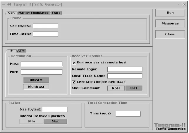
As shown in Figure 1 the user can specify the size L of the packets to be transmitted, the total generation time T, and the number of bytes for frame D. The amount of traffic is specified in terms of frames. (The word frame used in this paper should not be mistaken by the corresponding term used in the data protocol layer.) Clearly, the number of packets N generated per frame depends of frame size and
packet size, that is N=D L.
A remote application can be launched for collecting infor-mation about the transmitted traffic (Receiver Options in Figure 1). This information is stored into a trace file for latter processing. From the trace file, statistical measures can be evaluated such as: the probability mass function (pmf) of the jitter and its expected value, the pmf of the size of consecutive losses and the loss ratio, and the throughput.
Figure 1: Interface of trangram-II traffic generator
Packets from a frame can be transmitted in two forms: they are either sent one after another at the beginning of the frame generation interval or each packet is sent uni-formly spread over the interval.
It should be observed in Figure 2, for Generation Mode min, that the generation process sleeps between two con-secutive frames. In this case, after transmitting the last packet of a frame, the generator calculates the residual time till the beginning of the transmission of the next frame. If the residual time is positive, then a private
usleep() system call is executed, otherwise the next frame is transmitted immediately. Note that only one usleep()
system call is executed for each frame, and no busy wait is used. For Generation Mode max, the packets are transmit-ted uniformly over the interval between frames. In this case, the generation process sleeps after transmitting each Packet.
2.1
Generating Traffic from Models
The traffic generator tool can generate traffic from differ-ent models indicated bellow.
• CBR (Constant Bit Rate) traffic.
In this case, the generator transmits frames at constant
time intervals. The parameters that must be supplied are the total number of bytes per frame (Fsize), the time
in-terval between two frames (Ftime), and the packet size
as mentioned above.
• Markov Modulated Traffic.
The traffic is generated according to a continuous-time Markov reward model with finite states space. In this case a reward rate is associated to each state in the model. Let rj be associated to state j. Then the
transmis-sion rate when the model is at state j is rj bps. The
model can be specified using the Tangram-II modeling environment [3, 11], that generates the state transition rate matrix for the model and associated reward rates. (Any other tool can be used to generate the transition matrix, provided that the file format is that required by the generator.)
The traffic generator tool first obtains the state transi-tion probability between any two states as follows. Let
∆j be the sum of the output rates out of state j, that is,
∆j=
∑
kλj,k, where λj,k is the transition rate from state j
to k. Then the transition probability from state j to k is
Probj,k=λj,k
∆j
Figure 2: Generation modes
Assume that the system is at the state j. Since the amount of time in j is a random variable exponentially distributed with rate ∆j, a sample of this random variable is first
gen-erated. Clearly, the number of bytes that must be sent till be next transition is rj∗∆j. The traffic generator then
gen-erates a random sample to determine the next state from the state transition probabilities (the Pj,k) and the process
continues till the total generation time is reached.
• Traffic generated from a trace file.
The tool also allows the user to generate traffic base on a trace file where each line contains the amount of time from the last frame and the total number of bytes in the frame. It is important to note that the trace file can be obtained from a simulator or from any real multimedia data such as from a video coded in MPEG. The Tan-gram-II simulator is completely integrated with the traf-fic generator and, if this is the simulator of choice, the modeler can generate traffic with different charac-teristics including long range dependent traffic models such as FARIMA and FBM [7], Pareto, truncated Pareto and Weibul. Therefore, a wide range of options is available to the user.
3
Connection Admission Control (CAC)
Algorithms
Many connection admission control (CAC) algorithms have been proposed in the literature. Some authors classify the CAC algorithms into those based on traffic descriptors and those based on measurements [15, 10]. Others prefer to classify them by the different approximations to obtain the loss probability and the effective capacity [13]. There are also CAC algorithms for self-similar traffic models [16], and a few designed to work with specific scheduling policies [6]. There are schemes based on fluid models [8] and others that use Kalman filter to estimate the mean and variance of the instantaneous rate and the effective capac-ity [4].
Most of the CAC algorithms proposed are not of current practical use because either the parameters they require cannot be provided by the current ITU-T (International Telecommunication Union - Technical Committee) and ATM Forum standards or the calculations to be performed are too complex to be implemented in current network equipments
In the studies we present in section 5 we chose two CAC algorithms due to the following reasons:
• Algorithms based on standard ITU-T traffic descriptors. Although we realize that the traffic descriptors stand-ardized by the ITU-T (the usage parameters control (UPC)) do not capture relevant statistical characteristics of a multimedia source (e.g. second order statistics), we selected algorithms based on the standard UPC traffic descriptors because we want to analyze the behavior of these CAC algorithms through measurements made on a ATM switch, using the ATM traffic generator we de-veloped. Therefore, the user can only declare his/her traffic source using the UPC parameters.
• Applicability. The second reason is based on how sim-ple are the calculations performed. The algorithms should be based on sounding theoretical grounds and yet have calculations that are easy to perform and so easy to be implemented in a real switch.
In what follows we briefly survey the basic theory behind the CAC algorithms chosen for our experiments.
3.1 Effective Capacity: Unregulated Traffic
Consider a model where the bit rate generated by a num-ber of multiplexed connections is represented as a continu-ous flow of bits with intensity varying according to the state of an underlying continuous-time Markov chain. This model is called fluid flow model. The objective is to deter-mine the smallest value of the service rate C~, for a given
buffer size x that has to be allocated to the source model so that the QoS given by the buffer overflow probability is smaller than a tolerance ε. The value C~ is called the effec-tive capacity of the multiplexed connections.
t t-1
t-2 time
tx tx
Frame Frame
t t-1
t-2 time
tx usleep tx usleep
Frame Frame
Inter Frame time Inter Frame time
In order to calculate the effective capacity, the distribution of the buffer size as function of the traffic characteristics and transmission rate. This can be derived considering identical sources and for more general input Markov chains [14]. Unfortunately the computational complexity to calculate the effective capacity is not compatible with real-time requirements. In order to overcome this problem, approximations must be used.
Consider a model of one on-off source with parameters
λ,um,R, where λ is the rate transition from off to on, µ is the rate transition from on to off and R is the source peak rate.
The system of equations obtained from this model is given by:
D dF(x)
dx =QF(x) ,x≥ 0,
(1)
where,
D=
c 0
0 R−c
and Q=
−λ λ
µ −u
,
F(x) is the distribution of the buffer size.
The solution for system of equations (1) is given by 2, where zi and Φi are the eigenvalues and eigenvectors of
D–1 Q, respectively and the coefficients ai depend of
eigenvectors and initial conditions.
F(x)=
∑
i
aiΦiezix , x≥ 0 (2)
The largest negative eigenvalue of zi and the
correspond-ing eigenvector are used to obtain the overflow prob-ability. Calculating zi and the corresponding eigenvector
for the 2-state model above, and applying further assump-tions an explicit upper bound for the effective capacityC~
can be obtained (see [14] for details):
c
~ =αb(1 – ρ)R – x+√[αb(1 – ρ)R – x]
2
+ 4xαbρ(1 – ρ)R 2αb(1 – ρ)
(3)
where α= ln(1⁄ε), and b=1⁄µ. Note that when ρ→ 1 * b→∞ and taking limits in 3 yields the expected result
c
~ =R.
The linearity of equation 3 certainly simplifies how band-width is allocated to connections, but it also clearly identi-fies the limitations of the expression. In order to model the statistical multiplexing effects, the distribution of the sta-tionary bit rate is approximated by a Gaussian distribution. We obtain:
C~ = [m+α’σ] (4)
where α’ =√−2ln(ε) – ln(2π), m is mean aggregate bit rate
m=
∑
i=1
N
mi and σ is the standard deviation of the
aggre-gate bit rate σ2=
∑
i=1
N
σi2 . The combination of flow (3) and
stationary (4) approximations into a single expression gives the effective capacity of a set of connections. As both approximations overestimate the actual value of the desired effective capacity (flow approximation ignores the effect of smoothing gains with statistical multiplexing and stationary approximation ignores the size of buffer), the
effective capacity is chosen to be the minimum between the two approaches.
C~ = min
m+α’σ ,
∑
i=1N
c ~
i
(5)
where N is the number of multiplexed connections. This is the final expression used in our studies.
3.2 Effective Capacity: Regulated Traffic
In this approach all traffic sources are regulated by a leaky bucket, and more accurate bounds than those obtained for the non-regulated traffic can be obtained. Consider a model with N independent on-off traffic sources regulated by leaky bucket. The arrival rate of the regulated connec-tion j at a node is bounded by α(t)= min(Rjt , mjt+bj),
where Rj is the source peak rate, mj is the mean rate and bj
The effective bandwidth for a system that does not admit any loss, c0, can be obtained from the intersection of linear
equations c
C=
x
X and x=b – b(c – m)
R−m [5]:
c0=
R
1 +
X⁄C
b (R−m)
, ifm<bC x
m , otherwise
(6)
This result is an exact result if all sources are assumed identical, but conservative for heterogeneous sources.
In the second part of the approach, a small loss probability is considered. Chernoff’s bounds and asymptotic large de-viations approximation are used to obtain an estimate for
the loss probability: Ploss≤e−FK(s
∗
)
, where,
FK(s)=
sC –
∑
j=1N
Kj ln[1 – wj+wjesc0,j]
. The parameter Kj is the number of sources that can be admitted, s* is the
point where the function FK is maximized, wj is the
frac-tion of time that system is busy and equal to wj=m⁄c0j.
In the case of homogeneous sources (N= 1), s∗ is given by
s∗= 1
c0j ln
a
1 – a⋅
1 – w w
where a= (C⁄c
0j)⁄K, and
FK(s∗)=K a ln
a
w+(1 – a) ln 1 – a 1 −w
(7)
Equation (7) can be used to obtain kmax which is the value of K for which FK(s∗)= ln(1⁄ε), ε is the QoS requirement
(loss probability). Finally, the final expression for the sta-tistically-multiplexed effective capacity c~j for type j traffic
is:
c ~
j=
ln 1 –
wj
c0,j+
wj
c0,je
8∗c0,j
s∗+(ln(ε))⁄C
(8)
4
CAC Module
We have implemented for our test environment a module that emulates the two CAC algorithms outline above, and are useful to provide a basis for comparison against labo-ratory measurements and possible other CAC algorithms. The module calculates the Effective Capacity and the num-ber of admitted sources based on the CAC algorithms. The required parameters used by those algorithms are:
• The traffic descriptors;
• The buffer size, link capacity and the desired QoS.
The CAC module either operates as a network service or as a server that waits for requests, and it is associated with a configurable UDP port.
In server mode, the communication is established as shown in the Figure 3, where the socket BSD standards API, was used for communication with the client. This module is currently available for Linux Operational Sys-tems. Figure 3 shows a client (connection i) sending a re-quest to the CAC module server. This module either ac-cepts or rejects the incoming new connection according to the characteristics of the network node in addition with the specific CAC algorithm. If the client is accepted, the mod-ule sends an accept reply. Otherwise a reject packet is re-turned to the client.
The CAC module stores a list of clients currently admitted as indicated in Figure 3. When the client sends a discon-nect message to the server, the corresponding parameters stored in the server list are deleted, indicating that the allo-cated resources are released.
Figure 3: CAC module client-server communication
This module can be used to communicate with a number of applications such as a Video on Demand server. For that, the application needs only to communicate with the CAC server and supply the required data for the connec-tion.
5
Example Application of the Testbed
Developed
needed for the CAC algorithms is the buffer size allocated to the connection. Since the manufacturer specifications do not provide this information, neither indicates the algo-rithm used to allocate buffer to a connection, we develop a procedure that can be easily applied to determine this pa-rameter. To our knowledge this procedure is original, and general enough to be used in other switching equipments. Finally, we measure the QoS observed when traffic with different characteristics is generated by our generator and verify if the results produced by the CAC algorithms sur-veyed are consistent with the laboratory measurements.
5.1 Controlling the resources allocated to a
con-nection
The Fore-Systems ATM switch model ASX-1000 does not implement any CAC algorithm based on the theory we surveyed. The default admission control accepts a connec-tion if the sum of the declared peak rate of each source is smaller than the total available bandwidth shared by the connections. However, the switch has two configurable parameters available to the user. When their values vary, the number of admitted connections change as well as the total allocated capacity for the VBR sources. The purpose of this section is to evaluate the behavior of these so called “ overbooking” parameters and see if they can be adjusted to simulate the CAC algorithms surveyed.
As indicated in Table 1, we selected 4 types of traffic. The traffic parameters chosen are the same as those used in ref-erences [14] (for type 1 and 2) and [1] (for type 3 and 4).
Type of traffic
Peak Rate (Mbps)
Mean Rate (Mbps)
MBS (cells)
1 42.2 29.3 5000
2 4 2.1 366
3 6 0.15 25
4 1.5 0.15 250
Table 1: Selected traffic with different characteristics. (MBS = maxi-mum burst size.)
Each input traffic is associated with a VBR permanent vir-tual circuit (PVC). The switch accepts the creation of VBR PVCs associated to the same output port as long as the sum of the allocated capacity for each PVC is smaller than the total capacity of the port. The allocated capacity, however, can vary as a function of two configurable
pa-rameters in the switch: vbroverbooking (vbrob) and
vbrbufferoverbooking (vbrbuffob). The allocated capacity
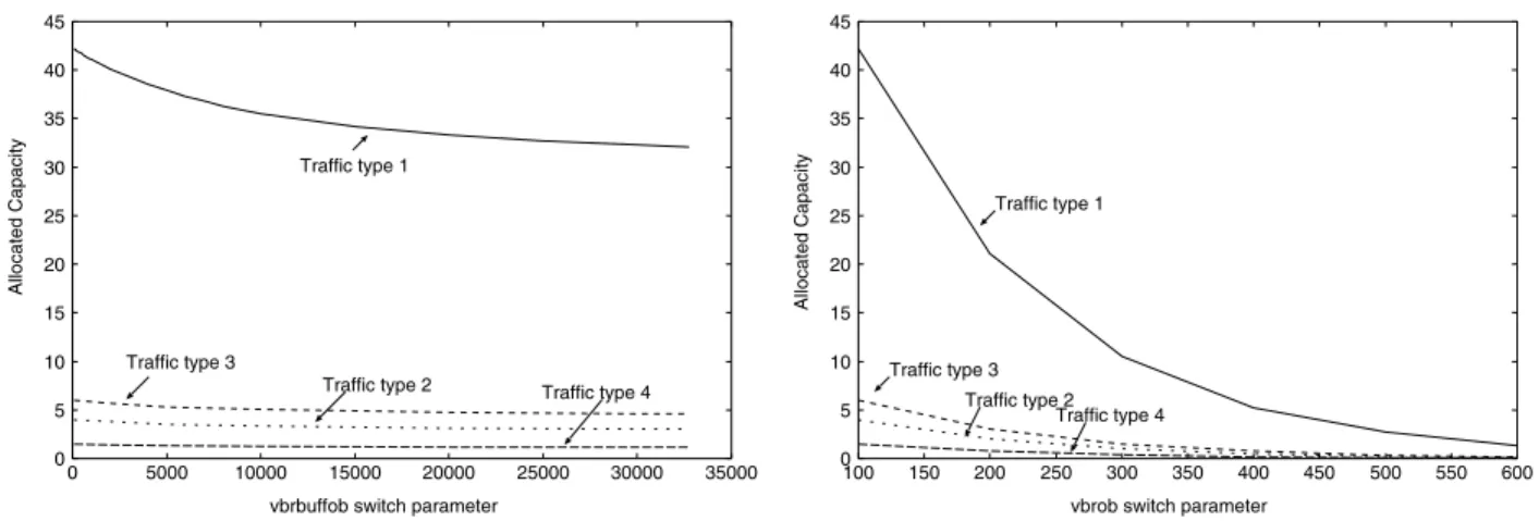
for the connection can be obtained by the user in the VPT (Virtual Path Terminator) section of the ATM switch. For example, if the parameters vbrob is p x 100, the current al-located capacity to each PVC is divided by p. The vbrbuf-fob parameter controls the buffer size for the connection, but no hints are given in the switch manual on how this parameter affects the allocated capacity and the buffer 2. Since the allocated buffer size is not available to the user, we developed a procedure to estimate this value, as it will be shown in the next section.
Figure 4 shows the allocated capacity as a function of each overbooking parameter. The term allocated capacity
is equivalent to the effective capacity in section 3. We use both terminologies here to differentiate what is given by the switch (allocated capacity as named in the switch manual) and what is calculated (effective capacity) by the CAC algorithms.
We can observe from the figures that the sensitivity of the
allocated capacity with respect to the vbrob is much larger than the sensitivity with respect to the vbrbuffob parameter that controls the allocated buffer size. This is consistent with the results obtained from the CAC algorithms. From section 3 we can verify that the effective capacity is a function of both the transmission rate as well as the buffer size, and its sensitivity with respect to the first parameter is much larger than that with the second parameter.
Note that we may think that the overbooking parameters may be configured to match both the allocated capacity
and the effective capacity calculated by a CAC algorithm. This is in principle possible, but requires the implementa-tion of a CAC algorithm and the knowledge of a network manager expert. Below we address the issue of matching both parameters and point to the possible difficulties.
The architecture of the ATM switch is based on a non-blocking shared-bus where each ATM port has transmis-sion capacity C=155 Mbps. According to the manufac-turer specifications, the output buffer size for a connection varies between 16 and 64 Kcells.
Figure 4: The allocated capacity versus the overbooking parameters of the Fore-Systems ASX-1000 ATM Switch
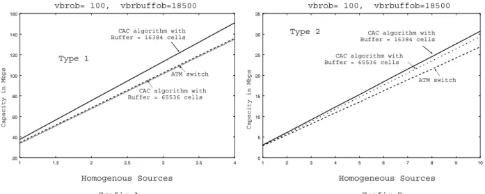
We first consider homogeneous sources and plot the effec-tive capacity for two different types of traffic sources. Since the actual buffer size is not available, we used the two extreme buffer sizes indicated in the manual. We chose the overbooking parameters to try to match the theo-retical value for the CAC algorithm used and that given by
the switch. The cell loss probability is specified as ε=10−5. From Figure 5 we can observe a relatively small discrep-ancy between the theoretical values and what is obtained by using a proper parameter value for the switch.
Figure 6 shows similar curves as above, but for heteroge-neous sources. We compare the admission regions of ATM switch and the CAC algorithm described in section 3 proposed by [5]. As shown in the figure, it is harder to choose the proper overbooking parameters for heterogene-ous sources than for homogeneheterogene-ous sources. (Although not shown in the figure we experiment with different
over-booking parameter values.) However, the tools
imple-mented can be used to help the choice, by using the results of the CAC module implemented.
5.2
Determining the Buffer size using the
Traffic Generator
In the previous paragraphs we mention that the actual buffer size allocated to a connection is not available to the user. The target switch implements Per-VC queueing, but no information is available concerning the algorithm used to allocate buffer space for each PVC. However, it is im-portant to be able to measure its value for the performance studies, including those we conduct here to show the ap-plicability of the testbed. In this section we devised a sim-ple procedure to measure the size of the buffer and applied this technique to the target ATM switch.
The basic approach taken to find the size of buffer is based on the cell loss process measured at the ATM switch port. The procedure we develop is as follows: we generate a CBR traffic during a period of time T. Clearly if the rate at which traffic is generated is above the transmission rate then cells will queue up at the switch output buffer allo-cated to the PVC. Suppose that traffic is generated at a rate
λ and the allocated capacity is C. Then cells are accumu-lated at the buffer at rate (λ – C) and no cells will be lost until the buffer fills up. Let τ be the amount of time neces-sary to fill up the buffer. Therefore, (λ – C)∗τ will be equal to the buffer size. Furthermore, after the buffer fills up, the cell loss rate is (λ−C) since traffic is generated at a constant rate.
Assuming that traffic is being generated during the period of time (0,t), if t<τ then no loss will be observed in (0,t). Let t1 and t2 be such that t2>t1>τ. Let l1 and l2 be the number of lost cells during (0 , t1) and (0 , t2),
respec-tively. Thus we must have l2 – l1
t2 – t1=λ−C, and we can eas-ily obtain λ−C and τ. Therefore,
buffersize=l2 – l1 t2 – t1t2 – l2
The approach is illustrated in Figure 7. That Figure shows the curve we should expect to obtain if we generate CBR traffic from (0 , t1) and (0 , t2) and measure a total cell loss of l1 and l2, respectively.
0 5 10 15 20 25 30 35 40 45
0 5000 10000 15000 20000 25000 30000 35000 0
5 10 15 20 25 30 35 40 45
100 150 200 250 300 350 400 450 500 550 600
vbrob switch parameter
Allocated Capacity
Traffic type 1
Traffic type 3
Traffic type 2 Traffic type 4
vbrbuffob switch parameter
Allocated Capacity
Traffic type 1
Traffic type 3
Figure 5: Effective capacity: homogeneous sources.
Figure 6: Effective capacity> heterogeneous sources.
Figure 7: Determining the buffer size.
Capacity in Mbps
20 40 60 80 100 120 140 160
1 1.5 2 2.5 3 3.5 4
Homogenous Sources
Grafic A
vbrob= 100, vbrbuffob=18500
Type 1
CAC algorithm with Buffer = 16384 cells
CAC algorithm with Buffer = 65536 cells
ATM switch
0 5 10 15 20 25 30 35
1 2 3 4 5 6 7 8 9 10
Capacity in Mbps
Homogeneous Sources
Grafic B
vbrob= 100, vbrbuffob=18500
Type 2
CAC algorithm with Buffer = 65536 cells
ATM switch CAC algorithm with Buffer = 16384 cells
0 200 400 600 800 1000 1200 1400
0 100 200 300 400 500 600 700 800 900
Number of sources type 4
Number of sources type 3
Comparative between admissable regions
ATM switch with vbrob=150, vbrbuffob=2800
Figure A
CAC Algorithm with
B=65536 cells, C=155 Mbps, PL=10-5
CAC Algorithm with B=16384 cells, C=155 Mbps,
PL=10-5
0 200 400 600 800 1000 1200 1400
0 100 200 300 400 500 600 700 800 900
ATM switch with vbrob=150, vbrbuffob=500
CAC Algorithm with
B=65536 cells, C=155 Mbps, PL=10-5
CAC Algorithm with B=16384 cells, C=155 Mbps, PL=10-5
Number of sources type 4
Figure B
Number of sources type 3
Comparative between admissable regions
l2
τ t1
total loss
time l1
t2
Now the approach is applied to the ATM switch. We re-call that we want to measure the amount of buffer allo-cated to a VBR connection by generating CBR traffic through the VBR PVC connection and measuring the re-sulting loss process. We have available 5 PCs to our ex-periment and since the output link is 155 Mbps, we gener-ate a CBR background traffic of 50 Mbps, and 4 CBR traf-fic of 26.8 Mbps with VBR contracts. The UPC contracts for the 4 VBRs PVCs have peak rate of 11.48 Mbps. This value was chosen so that we start observing losses after a period of approximately 5-6 seconds. Even though we generate CBR traffic, our contract is VBR, so we must choose the mean rate and maximum burst size for the con-nection. We also have to determine if these two last pa-rameters influence the buffer size allocated to the connec-tion. At each workstations, each traffic generator reserved a rate at the ATM PC card equal to the generated rate (26.8 Mbps).
Note that, according to Figure 8, the shape of the curves is as expected, that is, identical to Figure 7. From the proce-dure outlined above we calculate a total buffer size (for the four VBR connections) of 17805 cells with (3651) cells of confidence interval at 95% confidence level. We now vary the mean rate and MBS parameters and repeat the experi-ments. We have not observed any change in the measures performed and so we conclude that only the UPC peak rate influences the buffer size allocated to the connection.
Figure 8: Number of lost cells for each PVC as a function of time. (The traffic policing is disable at all ports of the ATM switch.)
In the last set of experiments we change the peak rate val-ues of the UPC contracts. (Recall that the mean rate and MBS have no influence in the results.) Figure 9 shows the results of the experiments. (This time, instead of plotting the average loss and confidence intervals of the set of measurements for each PVC, we plot a single sample for each PVC, to show the small variability of the results from each sample as compared to the mean.) For reference, we
indicate in the set of curves labeled A, a sample of the re-sults of the previous experiments (from Figure 8).
Figure 9: Number of lost cells for each PVC as a function of time: traffic with different UPC contracts. (The traffic policing is disabled at all ports of the ATM switch.)
The set of curves labeled B in Figure 9, shows the results when we set up 3 UPC contracts with peak rates identical to those in the experiments above, and increased the peak rate of the forth contract to R = 16.67 Mbps. We also maintain the background CBR contract of 50 Mbps. We observed no cell loss for the PVC with higher peak rate. The calculated total buffer size for the PVC that matained their peak rates is 14039 with 1603 confidence in-terval at 95% confidence level. From these results we see that an increase in the peak rate of a PVC contract leads to a decrease in the buffer allocated to the remaining VBR contracts.
Now we maintain two out of the three identical contracts above with the same peak rate and the third contract has its peak rate increased to R = 16.67 Mbps, that is two of the four PVC have higher rates that the remaining two. The set of curves C in Figure 9 displays the results. We observe no loss for the two PVC with highest peak rates. The calculated total buffer size of the remaining two PVCs is 12078 with 1680 confidence interval at 95% confidence level. As we can observe, increasing the number of con-tracts with relatively high rates reduces the total buffer al-located to the remaining contracts. This is consistent with our intuition, since we must reserve more buffer to con-tracts with higher rates.
5.3
Evaluating the Performance of CAC
Algorithms using our Traffic Generator
This section evaluates the performance of the two CAC al-gorithms surveyed. We also evaluated the usefulness of the overbooking parameters. In order to obtain the results 0
500 1000 1500 2000 2500 3000
0 2 4 6 8 10
Average cell loss
Time in seconds VC1 VC2 VC3 VC4
0 2000 4000 6000 8000 10000
4 5 6 7 8 9 10
Curves A Curves B Curves C
cell loss
we use the traffic generator we developed and its unique features to generate traffic with a variety of distinct char-acteristics. We also use the CAC module developed.
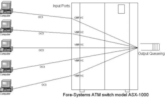
Figure 10 illustrates the testing environment. We have 5 workstations with ATM cards connecting to a ATM switch via OC3 (155Mbps). The ATM cards provide bandwidth allocation with guaranteed rate specified by user through the ATM API of each workstation. Each workstation has instances of the traffic generator tool sending data of a specified type. The rate allocated at each PC ATM card is equal to the peak rate of the correspond-ing PVC.
Figure10: Testing environment in our Laboratory
For the experiments, we first specify the input data needed for the CAC algorithm under study. These are the traffic descriptors, the switch characteristics (buffer size and link capacity) and the required QoS (cell loss probability). The CAC module then computes the number of traffic sources that can be admitted (assuming that all sources are homo-geneous) and the effective capacity of the aggregated traf-fic.
Second, we specify the model to be used by the traffic generator tool. In the experiments for this paper each traf-fic source model is identical to the one used in the original references for the CAC algorithms (Markov models).We choose to generate traffic where cells are uniformly spread during the active period.
Finally we create a UPC contract to represent each traffic source with descriptors identical to those given to the CAC module. Then we adjust the overbooking parameters so that the number of admitted sources is identical to that calculated by the CAC module.
We use the management interface available in the ATM switch for collect the number of lost cells. We reduced the capacity available to the VBR traffic by generating CBR
traffic as done in previous section. Therefore, the capacity
given to the CAC module is the OC3 capacity reduced by the CBR background rate. Furthermore, the buffer size used was obtained from the results of the previous section.
The traffic UPC contracts we used for the experiments are: peak rate equal to 11.48 Mbps, mean rate 5.50 Mbps and MBS of 1095 cells. Using a CBR background traffic of 120 Mbps, the available capacity to the VBR traffic is 30 Mbps (after discounting the signaling capacity as given by the switch). The measured buffer size is 17805. For a loss rate of 10−5, the effective capacity for each non-regulated source is c~i= 7.84, and the total aggregated capacity is
C~ = 23.5 Mbps. Only 3 VBR sources can be admitted, as indicated by the CAC algorithm for non-regulated traffic.
We generate traffic for periods of lengths 30, 60, 120, 300 and 600 seconds. When we setup the parameters of the ATM switch to vbrob = 150 and vbrbuffob = 100, to match the number of admitted sources given by the CAC module, we observe no cell losses. We only observed losses when 5 sources identical to those above generate traffic. (In order to admit 5 sources, the overbooking pa-rameter vbrob was changed to 200.) Figure 11.A, shows the fraction of cell loss obtained when 5 VBR sources are used. We can observe that, in this case, the cell loss rate was well above the specified. From this simple experiment we conclude that the CAC algorithm proposed by [14] is conservative, since the desired QoS was achieved even when one extra source was admitted.
The previous experiments was repeated, but now the po-licing mechanism (leaky-bucket) is enabled at all ATM ports. The ATM switch implements the standard mecha-nism GCRA (G eneric Cell Rate Algorithm) or leaky-bucket policing.
The theoretical CAC algorithm used was that proposed by [5]. In this case, the calculated effective capacity for each source is c~i= 5.49 Mbps, the aggregate effective capacity
is C~ = 27.45 Mbps, the CAC module indicates that up to 5 sources can be admitted.
The overbooking parameters of ATM switch were set to
Figure11: Fraction of lost cells per PVC.
From this experiment we conclude that if the CAC algo-rithm of [5] is applied, considering regulated sources, the required QoS is achieved.
Remarks: We should emphasize that the purpose of this section is only to show the applicability of the test envi-ronment we developed, and to indicate how the necessary parameters needed for the experiments can be obtained. We did not perform a careful evaluation of the CAC algo-rithms implemented, but only showed the results of a few test cases. For such a detailed evaluation we would need to further increase the number of admitted sources, generate other type of traffics, and generate much longer traces in order to be able to measure accurately very low loss prob-abilities. Although the tools developed can certainly per-form these jobs, we are limited by the number of stations with ATM boards in our laboratory. For instance, to
accu-rately measure loss rates in the order of 10−5 at 150 Mbps rates we would need approximately 50 minutes of meas-urements for each trace. However, our preliminary obser-vations (that include a few more tests than those reported here) indicate that the CAC algorithms surveyed are not very sensitive with respect to loss probabilities on the
or-der of 10−5, and that the algorithm of [5] for regulated traf-fic provides more accurate results than the algorithm of [14].
6 Summary
In this work we developed an environment useful for traf-fic engineering composed by a traftraf-fic generation and a CAC module tool. We exemplify its applicability by per-forming a number of tests using the Fore-Systems ATM switch model ASX-1000, to evaluate bandwidth manage-ment features and traffic policing. These tools are
cur-rently part of the Tangram-II modeling environment [3,11], available to download at the URL www.land.ufrj.br. Our contribution can be summarized as follows:
We developed a very flexible traffic generator that sup-portsUDP/IP or native-ATM (through the adaptation layer AAL5). This tool can generate packets (or cells) at vari-able intervals distributed according to the user specifica-tions. The tool supports CBR traffic, traffic generated ac-cording to a Markovian model or a trace file. It also pro-vides a traffic receiver to collect information about the re-ceived traffic, useful to evaluate a number of statistical measures. The following measures can be calculated: pmf of the jitter and its expected value, pmf of the number of consecutive losses and loss ratio, and throughput. The tool is completely integrated with the TANGRAM-II environ-ment. As such, Markov modulated traffic can be generated from TANGRAM-II models, or traffic traces for the gen-erator can be obtained directly from the TANGRAM-II simulator. Consequently complex traffic models can be used by combining modeling constructs with distributions such as FARIMA, FBM, Pareto, and others.
We developed a CAC module that emulates the two algo-rithms surveyed in section 3. The module computes the ef-fective capacity and the number of admitted sources for regulated and non-regulated traffic, from the traffic de-scriptors, link characteristics and QoS specified by the user. The CAC module can also operate as a server that waits for requests from clients at a UDP configurable port. As such, it can be easily coupled with other applications, such as a VoD server.
In order to demonstrate the applicability of the testbed de-veloped, we performed a number of experiments using an 0
0.02 0.04 0.06 0.08 0.1
0 100 200 300 400 500 600 0
0.02 0.04 0.06 0.08 0.1
0 100 200 300 400 500 600
VC1 VC2
VC3
VC4 VC5
Figure A Figure B
VC1
VC2 VC3 VC4 VC5 VC6
Fraction of cell loss
Time in seconds
Fraction of cell loss
ATM switch. In the experiments we evaluate the behavior of two, user configurable, admission control parameters. We also developed a technique to estimate buffer space al-located to a connection by generating traffic over a fixed interval and measuring the number of cells that were lost. To our knowledge this approach is original. Through the measurements performed, we were able to determine the buffer sizes shared by VBR connections and verified that the allocated space per PVC in the switch used for the ex-periments is a function of only the peak rate declared for the connections. Finally we made preliminary studies to evaluate the behavior of two CAC algorithms. The studies are aimed at demonstrating the applicability of the tools developed and should not be taken as a careful evaluation of each CAC algorithm.
Acknowledgement
This work is partially supported by grants from CNPq, CNPq/ProTem, Pronex and FAPERJ.
References
[1] A. Elwalid and D. Mitra. Effective Bandwidth of Gen-eral Markovian Traffic Sources an Amission Control of High-Speed Networks. IEEE ACM Transactions on Net-working, 1(3):329-343, 1993.
[2] W. Almesberger. High-speed ATM networking on low-end computer systems. In IEEE IPCCC 1996. IEEE Computer Society Press, 1996.
[3] R. M. L. R. Carmo, L. R. de Carvalho, E. de Souza e Silva, M. C. Diniz, and R. R. Muntz. Performance/Avail-ability Modeling with the TANGRAM-II Modeling En-vironment. Performance Evaluation, 33:45-65, 1998. [4] Z. Dziong, M. Juda, and L. G. Mason. A Framework for
Bandwidth Management in ATM Networks:Aggregate Equivalent Bandwidth Estimation Approach. IEEE ACM Transactions on Networking, 5(1):134-147, 1997. [5] A. Elwalid, D. Mitra, and R. H. Wentworth. A New
Ap-proach for Allocating Buffers and Bandwidth to Hetero-geneous Regulated Traffic in an ATM Node. IEEE Journal on Selected Areas in Communica-tions,13(6):1115-1127, 1995.
[6] R. G. Garroppo, S. Giordano, and M. Pagano. A CAC Algorithm for Per-VC Queueing Systems Loaded by Fractal Traffic. In Globecom-99, 1999.
[7] J. Beran, R. Sherman, M. S. Taqqu, and W. Willinger. Long-Range Dependence in Variable-Bit-Rate Video Traffic. IEEE Transactions on Communications, 43:1566-1579, 1995.
[8] G. Kesidis, J. Walrand, and C. S Chang. Effective Band-width for Multiclass Markov Fluids and other ATM sources. IEEE ACM Transactions on Networking, 1(4):424-428, 1993.
[9] T. Kurz, P. Thiran, and J. Y. Le Boudec. Regulation of a Connection Admission Control Algorithm. In Infocom-99, 1999.
[10] T. K. Lee and M. Zukerman. Efficiency Comparisons between different Model-Based and Measurement-Based Connection Admission Control Under Heavy Traffic. In Globecom-99, 1999.
[11] R. M. M. Leão, E. de Souza e Silva, and S. C. de Lucena. A Set of Tools for Traffic Modeling, Analysis and Ex-perimentation. In Proceedings of TOOLS’2000, pages 40-55, 2000.
[12] M. Leocádio and P. H. Aguiar Rodrigues. Uma Ferra-menta para Geração de Tráfego e Medição em Ambiente de Alto Desempenho. In SBRC-2000, 2000.
[13] H. G. Perros and K. M. Elsayed. Call Admission Control Schemes: A Review. IEEE Communications Magazine, 10(11):82-91, 1996.
[14] R. Guerin, H. Ahmadi, and M. Naghshineh. Equivalent Capacity and Its Application to Bandwidth Allocation in High-Speed Networks. IEEE Journal on selected areas in communications, 9(7):968-981, 1991.
[15] K. Shiomoto, N. Yamanaka, and T. Takahashi. Overview of Measurement-Based Connection Admission Control Methods in ATM networks }. IEEE Communications Surveys, 35, 1998.
[16] J. L Wang and A. Erramilli. A Connection Admission Control Algorithm for Self-Similar Traffic. In Globe-com-99, 1999.