Carlos H. F. dos Santos
Universidade Federal de Santa Catarina Departamento de Automação e Sistemas Departamento de Engenharia Mecânica Laboratório de Robótica Caixa Postal 476 Campus Universitário – Trindade 88040 900 Florianópolis, SC. Brazil [email protected]
Raul Guenther
Daniel Martins
Edson R. De Pieri
Virtual Kinematic Chains to Solve the
Underwater Vehicle-Manipulator
Systems Redundancy
This paper addresses the kinematics of the Underwater Vehicle-Manipulator Systems (UVMSs). Due the adittional degrees of freedom (dofs) provided by the vehicle, such systems are kinematically redundant, i.e. they possess more dofs than those required to execute a given task, and need to be solved using some redundancy technique. We present an approach based on introducing kinematic constraints. The approach uses the screw representation of movement and is based on the so-called Davies method used to solve the kinematics of closed kinematic chains. We describe the vehicle-manipulator system as an open-loop chain and present a virtual kinematic chain concept that allows closing this open chain. Applying the Davies method to this resulting closed chain, the UVMS direct kinematic is solved. The inverse kinematics is obtained using the same approach, by introducing extra constraints derived from energy savings requirements. The proposed approach is compared to another redundancy resolution method to illustrate the ability of the proposed strategy.
Keywords: UVMS , redundancy , screws, kinematic chains
Introduction
Underwater robotics is a technological field with increasing impact in the exploration of the ocean’s resources in the next decades. These systems are important in a number of shallow and deep-water missions for marine science, oil and gas, survey, exploration and military applications. Nowadays, most of the operations listed above are achieved by manned underwater vehicles or remotely operated vehicles; in case of manipulation tasks, those are performed resorting to remotely operated master/slave systems.
The use of manned vehicles is limited by two factors: cost and human risk. In hostile environments, remotely operated vehicles are an option but they demand a skilled operator to perform the task using a joystick. Beside the fact that the operator must be well trained, underwater communication is hard and a significant delay in the control is experienced. Because of this the aim of the research is to progressively make it possible perform such missions in a completely autonomous way (Antonelli, 2004).1
It is common to classify the underwater vehicles as Remotely Operated Vehicles (ROVs) and Autonomous Underwater Vehicles (AUVs). The term ROV denotes an underwater vehicle physically linked, via the tether, to an operator that can be on a submarine or on a surface ship. The tether gives power to the vehicle as well as closes the manned control loop. AUVs, on the other side, are supposed to be completely autonomous, thus relying to onboard power systems and artificial intelligence. These two types of underwater vehicles share some control problems and, sometimes are named Unmanned Underwater Vehicles (UUVs). In missions that require interaction with the environment, the vehicle can be equipped with one or more manipulators. In this case the system is usually called Underwater Vehicle-Manipulator System (UVMS).
Fossen (1994) is one of the first books dedicated to control problems of marine systems. The same author presents in (Fossen, 2002) an updated and extended version of the topics developed in the previous book. Antonelli (2003) is another book entirely dedicated to control problems of a manipulator mounted on a free floating underwater vehicle and, besides an extensive review, outlines that this subject is an emerging topic in research.
Presented at XI DINAME – International Symposium on Dynamic Problems of Mechanics, February 28th - March 4th, 2005, Ouro Preto. MG. Brazil. Paper accepted: June, 2005. Technical Editor: José Roberto de França Arruda.
In recent years, various research results have enabled the increasing of the vehicles autonomy by minimizing the need for the presence of human operators. A self-contained, intelligent, decision-making AUV is the goal of current research in underwater robotics. In this sense, Yuh and West (2001) present the state of the art of several existing AUVs and their control architectures. UVMSs are still under development. Several laboratories built some manipulation devices on underwater structures but very few of them can be considered as capable of autonomous manipulation (see Antonelli, 2004).
To perform underwater tasks in an autonomous way is challenging from the technological as well as from the theoretical aspects including the control of the UVMSs. Some facts that make it difficult to control UVMSs include the highly nonlinear dynamics, the uncertainties in the hydrodynamic coefficients, the ocean currents disturbances and the inherent kinematic redundancy of such systems.
A robotic system is kinematically redundant when it possesses more degrees of freedom (dofs) than those required to execute a given task. A generic manipulation task is usually given in terms of position/orientation trajectories for the end effector. In this sense, an UVMS is always kinematically redundant due to the dofs provided by the vehicle itself and so, its inverse kinematics (in which the vehicle-manipulator positions/orientations are calculated given end effector position/orientation) needs additional conditions to be solved.
It should be outlined, however, that the UVMSs are kinematically redundant systems whose movement has some particular characteristics. First, it is well known that it is not always efficient to use vehicle thrusters to move the manipulator end effector due to the difficulty of controlling the vehicle in hovering (Yoerger, Cook and Slotine, 1990). Moreover, due to the different inertias between vehicle and manipulator, movement of the latter is energetically more efficient. Thus, it is energetically efficient to keep the vehicle at rest during the task. However, to keep the vehicle at rest the thrusters must react to the ocean current whose strength exhibits a quadratic dependence on the relative velocity (Fossen, 1994). The UVMSs can easily recognize an ocean current and so, the vehicle can be aligned to the ocean current in order to minimize the energy dispended in the thrusters. These facts remark that the UVMS is a redundant system that has some kinematic constraints. This particular characteristic is explored in this paper.
(Canudas de Wit et al, 2000). This approach needs, however, the knowledge of the dynamic parameters, which are difficult to obtain due to the uncertainties in the hydrodynamic coefficients.
In this paper we focus our attention on the kinematic control of the UVMS. The goal is to find suitable vehicle/manipulator joint trajectories that correspond to a desired end effector trajectory. The output of this kinematic control provides the reference values to the dynamic control law of the UVMS. We consider the kinematic control independently of the dynamic control as in (Antonelli, 2003).
The kinematic control corresponds to obtain the inverse kinematics with the redundancy resolution. The simplest way to obtain the redundancy resolution of a kinematical system is to use the pseudoinverse of its Jacobian matrix (Sciavicco, 2004). In this case the inverse kinematic solution corresponds to the minimization of the vehicle/joint manipulator velocities in a least square sense. This approach is dimensional dependent (Davidson and Hunt, 2004) and the repeatability of the movement in the joints space is not guaranteed (Campos, 2004). Beside this, an approach based on the pseudoinverse (and, consequently, with the same limitations) named Task Priority Redundancy Resolution is widely used in the solution of the inverse kinematics of UVMSs (see Antonelli, 2003, and references therein). The Task Priority Redundancy Resolution technique considers explicitly the need of keeping the vehicle at rest as a second task priority.
In this paper we present a new approach to solve the redundancy of UVMSs. This approach is based on introducing kinematic constraints to the UVMS movements.
The additional kinematic constraints are introduced by imposing directly the vehicle velocities. To this end an open kinematic chain is used to represent the differential kinematics of the vehicle-manipulator system. Next, a virtual kinematic chain closes the open UVMS chain in order to allow the inverse kinematics of the resulting closed chain using the Davies method.
In this paper the vehicle velocities are imposed considering energy savings that result in aligning the vehicle to the ocean current and in keeping it at rest, as discussed above. The same approach can be used to increase of the system manipulability, as picked out in (Santos et al., 2006a, 2006b) and obstacles avoidance as detailed in (Guenther et al, 2004).
The remainder of this paper is organized as follows. First, we describe the movement of an UVMS. More specifically, we obtain the description of the UVMS manipulator end effector movement with respect to an inertial frame. In order to introduce a new approach to solve the inverse kinematics to this class of manipulators, the model of an UVMS using screws to represent its differential motion is presented. For completeness, the differential kinematics screw representation is shortly described. Next, we present the differential kinematics for a serial manipulator and a proposal to the vehicle differential kinematics using screws. By adding the vehicle/manipulator kinematics we came to the UVMS kinematics. Then we describe the Davies method and introduce the virtual kinematic chain concept. In the sequence our proposal to the UVMS direct and inverse kinematics is discussed. In order to compare our proposal with other redundancy resolution a brief description of the Singular Robust Task-Priority applied to the UVMS according to Antonelli (2003) is presented. Then we show and analyze simulations comparing the method presented in this paper to the Singular Robust Task-Priority in order to ilustrate our conclusions.
Nomenclature
$=screw movement or twist
h =pitch of the screw
Vp =linear velocity of point p
So= position vector of any point at the screw axis
$ˆ = normalized twist: a screw
S = normalized vector parallel to screw axis
N = matrix containing the normalized twists
T = transformation matrix of screw coordinates R = rotation matrix
W =skew-symmetric matrix representing a vector
q = manipulator joint angle
u = vehicle linear velocity in the x-direction
v = vehicle linear velocity in the y-direction
r = vehicle angular velocity in the z-direction
Greek Symbols
ω
= differential rotation about the screw axis, angular velocity
Ψ
= twist magnitude
Subscripts
s relative to secondary
p relative to primary
i,j relative to link or joint i,j
Screw Representation of Differential Kinematics
The screw is a geometric element (Fig.1), composed by a directed line (axis) and by a scalar parameter h with length dimension called pitch (see Davidson and Hunt, 2004, for example).
$
So
X Y
Z
O
S
Figure 1. Normalized screw.
If the directed line is represented by a normalized vector S (Fig.1), the screw is called normalized screw $ˆand is given by
× =
S S
S
o
...
$ˆ , (1)
where So is the vector directed from any point on the screw axis to
the origin of the reference frame O−XYZ. From this definition, it is noted that there are two vector components or six scalar components in the above screw representation. Notice that the vector So×S determines the moment of a line, the screw axis, around the origin of the reference frame.
A normalized screw $ˆ multiplied by a velocity magnitude Ψ (a scalar) is called a twist which represents an instantaneous movement of a rigid body with respect to an inertial reference frame, and could be given by
ω = Ψ =
P V
... $ˆ
$ , (2)
the body, which is instantaneously coincident with the origin of the XYZ
O− frame.
The movement between two adjacent links belonging to an n -link kinematic chain may also be represented by a twist. In this case, the twist represents the movement of link i with respect to link (i-1).
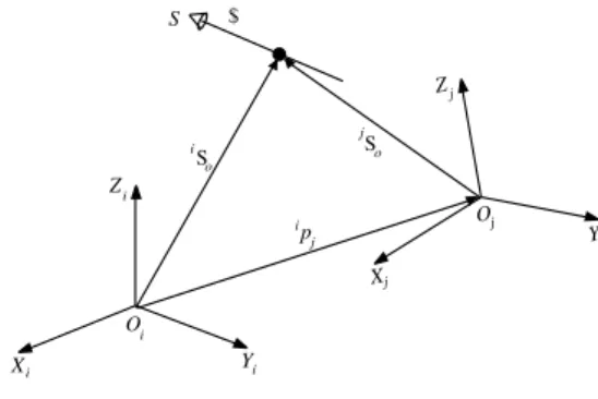
Often it is useful to represent the differential movement of a body, expressed by a twist $, in different reference frames. The coordinate systems transformation is done by the screw transformation matrix T (Tsai, 1999). Consider two reference frames of interest (Oi−XiYiZi) and (Oj−XjYjZj) as in Fig. 2.
$
ip j Z
Y X
Z
X
Y O
O
o S
i
So
j
S
j
j
j j
i
i i
i
Figure 2. Coordinate transformation of a screw.
The position of origin Oj relative to the Oi−XiYiZi frame is
given by ipj=[px,py,pz]T and the orientation of the Oj−XjYjZj
frame relative to the Oi−XiYiZi frame is described by a rotation
matrix iRj. A screw represented in the Oi−XiYiZi frame is denoted
by i$, and the same screw represented in the Oj−XjYjZj frame is
denoted by j$.
The matrix of transformation of screws between the jth frame and the ith frame ( $ j j$
i i =T
) is given by
=
j i j i j i
j i
j i
R R W
R
T 0 ,
−
− − =
0 0 0
x y
x z
y z
j i
p p
p p
p p
W , (3)
where j
iW
is the 3 x 3 skew-symmetric matrix representing the
vector ip
(expressed in the ith frame).
In the sequence, we present the manipulator and the vehicle kinematics in order to describe the UVMS kinematics.
Serial Manipulator Kinematics
For a serial manipulator, we may consider the movement of the end effector as being twisted instantaneously about the joint axes of an open-loop chain (Tsai, 1999). These instantaneous twists may be added linearly to give the resulting movement of the end effector. Consider, for example, the manipulator with six rotational joints showed in Fig. 3. For this manipulator the differential kinematics may be written as
∑
= Ψ = 6
1 $ˆ $
i
mi mi B E
B , (4)
where B$ˆmi is the manipulator i-th normalized screw described in the base frame (B-frame in Fig.4), Ψmi is the correspondent i-th
magnitude and B$E is the screw that represents the end effector’s movement in the B-frame.
B
Z
B
X
B
Y $m1
$m2
$m3 $m4 $m5
$m6
Figure 3. The serial manipulator.
With the objective to present the movement of a manipulator on a vehicle, the next section describes the differential kinematics of a vehicle in a suitable form to be added to the manipulator differential kinematics given above.
Vehicle Differential Kinematics
We may consider the movement of a rigid body as being twisted instantaneously about several screw axes. These screws form a screw system whose order is defined by the number of linearly independent screws that spans the system (Tsai, 1999). A vehicle has, in general, six degrees of freedom and so, its movement may be represented by a screw belonging to a sixth order screw system ($V). In other words, six independent screws may span the vehicle movement, i.e.,
∑
= Ψ = 6
1
$ˆ $
i vi vi
V , (5)
where $ˆvi is the i-th normalized screw and Ψvi is the i-th amplitude.
It should be outlined that, in case the set of normalized screws
} 6 , , 1 ,
{Ψvi i= … is linearly independent, Eq.(5) represents the
general vehicle motion as well as describes the movement of an open-loop chain with six links and six kinematic pairs (joints) each one with only one degree-of-freedom.
Using Eq. (5) to describe the vehicle’s movement, we may choose an open-loop chain with three orthogonal prismatic (P) joints and a spherical (S) one (Fig. 4) in order to represent the movement in a Cartesian reference frame as in (Campos et al, 2005). The first joint of this chain is prismatic and allows the movement between the first link and the base along the X-axis. It is named px and its movement is represented by the normalized screw $ˆpx. The second
and the third joints are prismatic, allow the movement between the second and the first, and between the third and the second links, along the Y-axis (py) and the Z-axis (pz), respectively, and are represented by the normalized screws $ˆpy and $ˆpz. The spherical
joint may be instantaneously changed by three rotational joints in the X, Y and Z directions (rx, ry, rz) and its movement are represented by the normalized screws $ˆrx, $ˆry and $ˆrz. Due to its
$px $py
$pz
Yc
Zc Xc $rx ,$ry ,$rz) ( S Y X Z C-Frame
Figure 4. Vehicle movement represented by an (PPPS) open kinematic chain.
The screws representing the PPPS chain independent movements are expressed in the simplest form if we choose a reference frame attached to the link that connects joints pz and rx
(the first rotational joint of the spherical joint), designated as C-frame in Fig. 4, to denote a suitable Cartesian reference C-frame. Using Eq.(2) we obtain (Campos et al, 2005):
T pz C T py C T px C T rz C T ry C T rx C ) 1 , 0 , 0 ; 0 , 0 , 0 ( $ˆ , ) 0 , 1 , 0 ; 0 , 0 , 0 ( $ˆ , ) 0 , 0 , 1 ; 0 , 0 , 0 ( $ˆ ) 0 , 0 , 0 ; 1 , 0 , 0 ( $ˆ , ) 0 , 0 , 0 ; 0 , 1 , 0 ( $ˆ , ) 0 , 0 , 0 ; 0 , 0 , 1 ( $ˆ = = = = = = (6)
This normalized screws set is even linearly independent and represents the vehicle motion in the C-frame. In practice the vehicle movement is usually described in a frame located at the vehicle gravity center with the axes directed according to its principal inertia directions, here named as vehicle frame (V-frame). To obtain the vehicle movement description in this V-frame, we may use the matrix of screws transformation between the C-frame and the
V-frame given in Eq. (3), i.e., C V
C V V
V$ = T $ , where
∑
= Ψ = 6 1 $ˆ $ i vi vi C VC , (7)
and C px
v C$ˆ $ˆ
1= , py
C v C$ˆ $ˆ
2= , pz
C v C
$ˆ
$ˆ3= , rx
C v
C$ˆ $ˆ
4= , ry
C v C
$ˆ $ˆ5= ,
rz C v
C$ˆ $ˆ
6= , where the normalized screws $ˆpx, $ˆpy , $ˆpz, $ˆrx$ˆry
and $ˆrz, are given in Eq. (6).
The origin of the C-frame is chosen coincident with the origin of the V-frame. Therefore, the position vector of one origin with respect to the other is null as well as the matrix W given in Eq.(3).
The matrix of screws transformationV C
T is obtained calculating the rotation matrix between the C and V frames (V C
R ). To this end it
should be observed that the C-frame was chosen parallel to the
inertial frame (I-frame) and so, I V
V C
R
R = , where IRV is the rotation
matrix that gives the orientation of the vehicle in the I-frame commonly measured in the RPY (Roll-Pitch-Yaw) angles (Antonelli, 2003). By transposing CRV we obtain
C VR that is
substituted in Eq.(3) to calculate VTC and, using Eq.(7) results
∑
= Ψ = 6 1 $ˆ $ i vi vi C C V VV T . (8)
The UVMS Kinematics
In an UVMS, the manipulator has a mobile base. So, the manipulator end effector movement with respect to an inertial frame is obtained by adding the manipulator end effector movement with respect to its base to the base movement (Fig. 5), i.e.,
E B B I V I E I T $ $
$ = + , (9)
where B
I
T is the matrix of screws transformation between the base manipulator frame and the considered inertial frame.
Y X
Z
$ν1 $ν2
$ν3
S($ν4,$ν5,$ν6)
ν ν Zν X Y B X B Z B Y
$m4$m5
$m6
$m1
$m2
$m3
Figure 5. An Underwater Vehicle-Manipulator System.
Let an inertial frame instantaneously coincident with the vehicle frame (V-frame) defined above. In this case Eq.(9) results
∑
∑
=
= Ψ + Ψ
= 6 1 6 1 $ˆ $ˆ $ i mi mi V i vi vi V E V (10)
where C vi
C V vi V
T $ˆ
$ˆ = , i = 1,…,6, and R mi
R B B V mi
V$ˆ = T T $ˆ .
Eq.(10) may be rewritten as
Ψ =J
E V
$ , (11)
where,
[
$ˆ1 $ˆ2 ... $6 $ˆ1 $ˆ 2 ... $ˆm6]
V m V m V v V v V v VJ= , (12)
[
]
Tm
m1 6
6
1 Ψ Ψ Ψ
Ψ =
Ψ ν … ν … . (13)
Eq. (11) expresses the UVMS kinematics as an open-loop chain constituted by the manipulator chain attached to the vehicle chain. It should be observed that the matrix J in Eq.(11) has six rows and twelve columns and outlines the system redundancy.
In this paper, we present a new methodology to invert the UVMS kinematics (Eq.(11)) derived from the Davies Method and the virtual kinematic chain concept described in the sequence.
Davies Method
Davies method is a systematic way to relate the joint velocities in closed kinematic chains. It is based on the so-called Kirchhoff-Davies circulation law (Kirchhoff-Davies, 1981, 2000). Kirchhoff-Davies solves the differential kinematics of closed kinematic chains from the Kirchhoff circulation law for electrical circuits. The Kirchhoff-Davies circulation law states that “The algebraic sum of relative velocities of kinematic pairs along any closed kinematic chain is zero”' (Davies, 1981).
Using this law, the relationship among the velocities of a closed kinematic chain may be obtained in order to solve its differential kinematics, as is presented in (Santos et al , 2005) and (Guenther et al., 2005).
where 0 is a zero vector which dimension corresponds to the dimension of twists $i.
According to the normalized screw definition (Hunt, 2000) this equation may be rewritten as
∑
= = Ψ
n
i i i
1
0
$ˆ , (15)
where $ˆi represents the normalized screw of twist $i and Ψi
represents the velocity magnitude of the twist i. Eq. (15) is the constraint equation which, in general, could be written as
0
= Ψ
N , (16)
where N is the network matrix containing the normalized screws which signs depend on the screw definition in the circuit orientation, and Ψis the magnitude vector. A closed kinematic chain has active (or actuated) joints, here named primary joints, and passive joints, here named secondary joints. The constraint equation, Eq. (16), allows to calculate the secondary joint velocities as functions of the primary joint velocities. To this end, the constraint equation is rearranged highlighting the primary and the secondary joint velocities and Eq. (16) can be rewritten as follows:
[
]
... =0
Ψ Ψ
p s
p s N
N ⋮ , (17)
where Np and Ns are the primary and secondary network
matrices, respectively, and Ψp , Ψs are the corresponding primary
and secondary magnitude vectors, respectively.
This equation may be rewritten as NsΨs =−NpΨp and the
joint space kinematic solution is given by
p p s s =−N N Ψ Ψ −1
(18)
This outlines that the Davies method constitutes a systematic way to express the joint rates of passive joints as functions of the joint rates of the actuated joints in closed kinematic chains.
In the next section, we introduce the virtual kinematic chain concept, which allows closing open kinematic chains in order to apply the Davies method.
The Virtual Kinematic Chain Concept
The virtual kinematic chain, virtual chain for short, is essentially a tool to obtain information about the movement of a kinematic chain or to impose movements on a kinematic chain.
In this paper, we use the virtual kinematic chain concept introduced by Campos (2004), who defines a virtual chain as a kinematic chain composed by links (virtual links) and joints (virtual joints) satisfying the following three properties: a) the virtual chain is open; b) it has joints whose normalized screws are linearly independent; and c) it does not change the mobility of the real kinematic chain.
Either to obtain information about the movement of a (real) chain or to change its movement, we apply virtual chains to close open real chains. All the kinematic chains that satisfy the three properties cited above may be used as virtual kinematic chains. A particularly useful virtual chain is the orthogonal PPPS chain
presented in (Fig. 4) and described in vehicle differential kinematics section.
In the next two sections, this PPPS chain is used to close the UVMS open-loop chain in order to obtain information about the end effector motion in a Cartesian frame and to impose movements to the UVMS chain.
UVMS Direct Kinematics
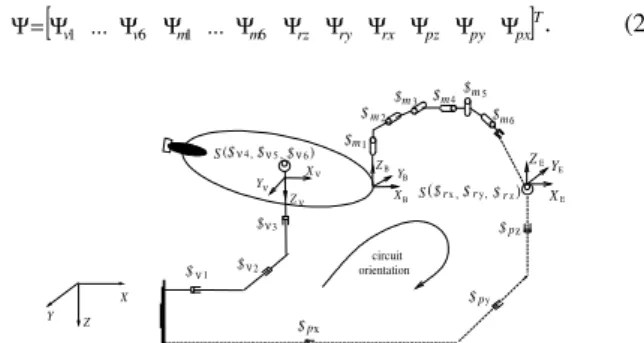
The end effector movement description in a Cartesian frame may be obtained closing the UVMS chain by introducing a PPPS virtual chain between the base and the end effector as in Fig. 6. In this case, regarding the circuit orientation indicated in the figure, the closed-loop chain network matrix is given by
[
v v m m rz ry rx pz py px]
N=$ˆ1 ...$ˆ6 $ˆ1 ...$ˆ6 −$ˆ −$ˆ −$ˆ −$ˆ −$ˆ −$ˆ , (19)
where the superscript V indicating that all the normalized screws are represented in the vehicle frame is omitted for simplicity. The negative terms in Eq. (18) are in accordance with the definitions of the screws that represent the virtual joint motions given in the section which describes the vehicle differential kinematics. The corresponding magnitude vector is
[
]
Tpx py pz rx ry rz m m v
v Ψ Ψ Ψ Ψ Ψ Ψ Ψ Ψ Ψ
Ψ =
Ψ 1 ... 6 1 ... 6 . (20)
Y X Z
$ν3
ν
$ 1 $ν2 orientation circuit
ν4$ν5
$ , ,$ν6) (
S
ν
Zν ν
X Y
$m2
$m3 $m4$m5
$m6
S($rx,$ry,$rz)
B
X
B
Y
B
Z YE
XE
ZE
p $y
pz
$
p $x
$m1
Figure 6. The Underwater Vehicle-Manipulator System with the PPPS virtual chain.
To solve the direct kinematics, we select the velocities magnitudes corresponding to the UVMS as the components of the primary vector Ψp and the magnitudes of the operational space
(represented by the virtual kinematic pairs) as the components of the secondary vector Ψs. The corresponding primary and secondary
matrices result
[
$ˆv1 $ˆv6 $ˆm1 $ˆm6]
p
N = … … (21)
[
rz ry rx pz py px]
s
N =−$ˆ −$ˆ −$ˆ −$ˆ −$ˆ −$ˆ . (22)
The magnitudes of the secondary kinematic pairs, i.e., the end effector velocities in the Cartesian frame, are calculated using Eq. (18), in which the secondary matrix needs to be inverted. It should be remarked that the secondary matrix has always full rank in this case, as can be observed in the Eq. (6), and so it is always invertible.
UVMS Inverse Kinematics
To obtain the vehicle and the manipulator velocities once given the end effector velocities (inverse kinematics), we select the operational space (virtual kinematic pairs) as the components of the
primary magnitude vector Ψp and velocity magnitudes
magnitude vector Ψs. In this case, the primary and the secondary
matrix result
[
rz ry rx pz py px]
p
N = −$ˆ −$ˆ −$ˆ −$ˆ −$ˆ −$ˆ , (23)
[
$ˆv1 $ˆv6 $ˆm1 $ˆm6]
s
N= … … . (24)
Again, to calculate the magnitudes of the secondary pairs, we need to invert the secondary matrix. Matrix Ns cannot be inverted because it has twelve columns and only six rows. We must specify six supplementary velocity magnitudes and include it in the primary magnitude vector in order to obtain a secondary matrix that could be inverted or, alternatively, we need to introduce six additional kinematic constraints.
The velocity magnitudes may be specified considering, for example, energy savings, i.e., reduce energy consumption. This energy savings could be achieved by keeping the vehicle aligned with the ocean current as suggested by Antonelli (2003). Correspondingly, this could be done by specifying the rotation components of the vehicle velocities in order to keep the vehicle aligned with the ocean current and making its linear velocities to be equal zero.
The primary and the secondary matrix result
[
$ˆrz $ˆry $ˆrx $ˆpz $ˆpy $ˆpx $ˆv1 $ˆv6]
p
N =− − − − − − … , (25)
[
$ˆm1 $ˆm2 $ˆm3 $ˆm4 $ˆm5 $ˆm6]
s
N = . (26)
This secondary matrix could be inverted even if it is full rank, i.e. even if the kinematic chain is not at a singularity. This outlines the easiness of obtain the inverse kinematics allowed by the approach proposed in this paper only by adequately the primary velocity magnitudes.
Due to the use of screws to represent the involved movements, this approach allows also to choose reference frames where this representation is simpler and so, the secondary matrix Ns is sparser
and, consequently, easier to be inverted. This easiness of invertion makes the algorithm for motion coordination more efficient as it was verified in simulations by Santos and Guenther (2004) and Santos et al (2005).
Singular Robust Task-Priority applied to the UVMS
According to Liégeois, (1977) the inverse kinematics of a redundant mechanism can be solved in terms of a minimization problem of a quadratic cost function. In the case of the UVMS, this function is constructed from the manipulator and vehicle joint velocities vector, and give the follow general solution:
(
)
(
s N p p) (
sd s p pd)
d p
px J I J J x J J x
J ɺ , ɺ, ∗ɺ ,
∗ ∗
∗ + − −
=
ς , (27)
where, xɺp,d, xɺs,d, Js, Jp, J∗p are the primary velocity, the
secondary velocity, the secondary Jacobian, the primary Jacobian and the Pseudoinverse (denoted by ∗ in this work) primary Jacobian respectively. Equation (27) represents the Task-Priority redundancy resolution.
However, for this solution, the problem of the algorithmic singularities still remains unsolved. In this case, it is possible to experience an algorithmic singularity when Js and Jp are full
rank but the matrix Js
(
IN−Jp∗Jp)
drop rank. In order to overcomethis problem, a robust solution to the occurrence of the algorithmic singularities is based on the following mapping (Antonelli, 2003):
(
)
, .,d N p p s sd
p
px I J J J x
J∗ɺ + − ∗ ∗ɺ
=
ς (28)
This algorithm has a geometrical interpretation: both tasks are separately inverted by the use of the pseudoinverse of the corresponding Jacobian; the joint velocities associated with the secondary task are further projected in the null space of the primary task Jp.
Simulation Results
This section presents the simulation results for a task performed using both the Singular Robust Task-Priority and the Kinematic Constraint approach presented in this paper.
The UVMS model is based on a real model of a UVMS showed in (Antonelli and Chiaverini , 1998, Antonelli, 2003). The vehicle has a length of 5 meters and each link of the manipulator has a length of 2 meters. For the sake of clarity we have restricted our attention to a planar task described in the plane of the manipulator, that is mounted horizontally, as in (Antonelli, 2003). Furthermore, this choice helps the comparison of the results.
Figure 7. UVMS initial configuration.
Let the initial configuration of the vehicle be: x=0m,
0
y= m, ψ=0rad and the manipulator joint angles be: q = [q1 q2 q3 ]T = [1.47 –1 0.3]T rad, corresponding to the end-effector location: xE=5.92 m, yE=4.29m, ψE=0.77rad (see Fig. 7).
As showed in Fig. 8, the task consists in aligning the vehicle with the ocean current orientation, here considered equal to 0.78 rad, and, simultaneously, making the end effector perform two returns in a circumference of 1 meter of diameter during a period of 10 seconds.
This simulation uses an integration step of 0.1 seconds with the Euler method (Burden, 2003).
In the Singular Robust Task-Priority method the movement of the end effector is performed in order to minimize the vehicle movements. The corresponding simulation results are shown in Figs. 9 to 11. Figure 9 shows the x, y and phi (angle around the z-direction which defines the orientation) vehicle positions. Figure 10 shows the manipulator joint angles q1, q2 and q3. Figure 11 reports the vehicle linear velocities u (in the x-direction) and v (in the y-direction), and the angular velocity r (in the z-direction).
The results in Figs. 9 and 11, outline that, despite the Task-Priority approach minimizes the vehicle movement, it does not keep the vehicle at rest as intended. This fact is a consequence from the minimization on which the approach is based.
In the kinematic constraint approach proposed in this paper, the vehicle is kept at rest by imposing the corresponding kinematic constraint in terms of velocity magnitudes. The simulation results are shown in Fig. 12 (vehicle positions and orientation), Fig. 13 (manipulator joint positions) and Fig. 14 (vehicle velocities).
By comparing the manipulator joint positions obtained with the Task-Priority approach (Fig. 10) and the manipulator joint positions calculated using the kinematic constraint approach (Fig. 13), it could be observed that they are similar.
Figures 12 and 14 shown that using the kinematic constraint approach the vehicle is kept at rest as desired.
These results illustrate that the undesirable vehicle movements resulting from the Task-Priority approach could be avoided by imposing kinematic constraints.
The vehicle-manipulator positions and velocities obtained are the outputs of the UVMS kinematic control and, consequently, the inputs to the UVMS dynamic control. This means that the undesirable vehicle movements which excite the system dynamics unnecessarily could be avoided by the approach proposed in this paper.
Figure 9. Singular Robust Task-Priority: vehicle positions and orientation.
Figure 10. Singular Robust Task-Priority: manipulator joint angles.
Figure 11. Singular Robust Task-Priority: linear and angular vehicle velocities.
Figure 12. Kinematic Constraint Approach: vehicle positions and orientation.
Figure 13. Kinematic Constraint Approach: manipulator joint angles.
Conclusions
This paper presents a new approach to the kinematic control of
Underwater Vehicle-Manipulator Systems (UVMSs). This
kinematic control consists in obtaining the inverse kinematics of this kind of redundant system, which is used as an input to its dynamic control.
The presented approach is based on introducing directly some kinematic constraints intrinsic to this kind of systems, and is derived using the screw representation of the differential kinematics of rigid bodies, the Davies method and a virtual kinematic chain concept.
In order to enable an easy adding of the vehicle and manipulator movements, a suitable form of the vehicle kinematics is introduced.
By modeling the UVMS as an open kinematic chain and closing this chain with a virtual chain, it is shown that the kinematic constraints could be introduced directly by imposing the corresponding velocity magnitudes in this closed chain.
This approach avoids undesirable vehicle movements generated as inputs to the dynamic control, always present in the usual approaches based on the minimization of some cost function.
In this sense, the presented approach avoids undesirable system dynamics excitation, as the simulations have shown.
Simulations illustrate these results.
Acknowledgements
This work has been partially supported by “Conselho Nacional de Desenvolvimento Científico e Tecnológico” (CNPq), Brazil.
References
Antonelli, G., 2004, “Open Control Problems in Underwater Robotics”,
Fourth International Workshop on Robot Motion and Control, June 17-20, Puszczykowo, PL, pp. 219--229.
Antonelli, G., 2003, “Underwater Robots – Motion and Force Control
of Vehicle-Manipulator Systems”, Springer-Verlag Berlin, Germany. Antonelli, G. and Chiaverini, S. 1998, “Task-Priority Redundancy
Resolution for Underwater Vehicle-Manipulator Systems”, In: IEEE
International Conference on Robotics and Automation, Leuven, Belgium, 768-773.
Burden, R.L., Faires, J.D., 2003, “Numerical Analysis”, Thompson
Learning, São Paulo SP.
Campos, A.B., Martins, D. and Guenther, R., 2004, “Differential
Kinematics of Robots Using Virtual Chains”, Mechatronics & Robotics
2004, Aachen, Germany, 13-15 September.
Campos, A.B., Martins, D. and Guenther, R., 2005, “Differential
Kinematics of Serial Manipulators Using Virtual Chains”, Journal of the
Brazilian Society of Mechanical Sciences and Engineering, vol. XXVII, no. 4, pp. 345-356.
Canudas de Wit, C., Olguin Diaz, E., Perrier, M., 2000, “Nonlinear Control of an Underwater Vehicle/Manipulator System with Composite
Dynamics”. IEEE Transactions on Control System Technology 8:948-960.
Davies, T. H., 1981, “Kirchhoff's circulation law applied to multi-loop
kinematic chains”, Mechanism and Machine Theory 16: 171-183.
Davies, T. H., 2000, “The 1887 committee meets again. subject:
freedom and constraint”, in H. Hunt (ed.), Ball 2000 Conference, University
of Cambridge, Cambridge University Press, Trinity College, pp. 1-56.
Davidson, J.K., Hunt, K.H., 2004, “Robots and screw theory”, Oxford
University Press, New York.
Fossen, T. I, 2002. “MarineControl Systems: Guidance, Navigation and
Control of Ships, Rigs and Underwater Vehicles”. Marine Cybernetics AS. Trondheim , NO.
Fossen, T. I, 1994. “Guidance and Control of Ocean Vehicles”. John
Wiley & Sons. Chichester, UK.
Hunt, K. H., 2000, “Don't cross-thread the screw”, in H. Hunt (ed.), Ball
2000 Conference, University of Cambridge, Cambridge University Press, Trinity College, pp. 1-37.
Liégeois, A, 1977, “Automatic Supervisory Control of the Configuration
and Behavior of Multibody Mechanisms”, in IEEE Transactions of Systems,
Man and Cybernetics 7:868-871 .
Guenther, R., Simas, H. and Martins, D., 2004, “A Redundant
Manipulator to Operate in Confined Spaces”, VI Induscon, Joinville, Brazil,
12-15 October.
Guenther, R., Santos, C.H.F., Martins, D., De Pieri, E.R., 2005, “A new
approach to the underwater vehicle-manipulator systems kinematics”, XI
Diname, Ouro Preto, Brazil, Febrary 28 – March 4.
Santos, C.H. and Guenther, R., 2004, “The Inverse Kinematics of
Underwater Vehicle-Manipulator Systems”, Technical Report, Robotics
Laboratory, UFSC, Florianópolis, SC, Brazil.
Santos, C.H., Guenther, R., Martins, D., De Pieri, E.R., 2005, “Inverse kinematics of the underwater vehicle-manipulator systems using kinematic
constraints”, in 11th IEEE Int. Conf. on Methods and Models in Automation
and Robotics, Miedzyzdroje Poland, August 2005.
Santos, C.H., Guenther, R. and De Pieri, E.R., 2006a, “A reactive neural network architecture to redundancy resolution for underwater
vehicle-manipulator systems ”, in press, IEEE International Conference on Robotics
and Automation, Orlando, USA.
Santos, C.H., Bittencourt, G., Guenther, R. and De Pieri, E.R., 2006b, “A fuzzy hybrid singularity avoidance for underwater vehicle-manipulator
systems”, in press, 12th IFAC Symposium on Information Control Problems
in Manufacturing, Saint Etienne, France.
Sarkar, N. and Podder, T.K., 2001, “Coordinated motion planning and control of autonomous underwater vehicle-manipulator systems subject to
drag optimization”. IEEE Journal of Oceanic Engineering 26(2), 228-239.
Sciavicco, L., Siciliano, B., 1996, “Modeling and control of robot
manipulators”, The McGraw-Hill Companies, Inc.
Tsai, L.-W., 1999, “Robot Analysis: the Mechanics of Serial and
Parallel Manipulators”, John Wiley & Sons, New York.
Yoerger, D.R., Cooke, J.G. and Slotine, J.J.E., 1990, "The influence of thruster dynamics on underwater vehicle behavior and their incorporation
into control system design", IEEE Journal of Oceanic Engineering, Vol. 15,
No. 2, 167-178.
Yuh, J., 2000, “Design and Control of Autonomous Underwater Robots:
A Survey”, in: Autonomous Robots 8, pp. 7-24.
Yuh, J. and West, M. , 2001, “Underwater Robotics”. Journal of