Harry Edmar Schulz
[email protected]Geraldo Lombardi
[email protected]Francisco Júlio do Nascimento
[email protected]Hélio José Donizeti Trebi
[email protected]Jorge Nicolau dos Santos
[email protected]André Luiz Andrade Simões
[email protected]University of São Paulo Nucleus of Thermal Engineering and Fluids Dept. of Mechanical Engineering and
Lab. of Transport Phenomena Dept. of Hydraulics and Sanitary Engineering School of Engineering at São Carlos 13566-590 São Carlos, SP, Brazil
Usable Work of Macro-Scale Cavities
in Liquids
It is shown that the generation of cavities in a liquid can produce usable work, which is illustrated by the stretching of a string. This work is done during the expansion of the cavity, and not with its collapse. Basic equations are presented for the movement of a device moved by the so called cavity events. A theoretical solution is also proposed, which uses polynomial functions relating the so called “excess of pressure” in the cavity and time. Evaluations of the force generated during the expansion of the cavity showed a mean peak value of about 58 N for the moving container, while measurements with the container fixed to a support showed a peak value of 476 N, considered somewhat overestimated, because high frequency oscillations seem to superpose the mean behavior. Simultaneous phenomena occurring during the cavity events are also described. Series of pictures of the experiments are presented.
Keywords: macro-scale cavities, bubble dynamics, ebullition, cavities’ work
Introduction1
Cavitation is the term used to describe the formation, behavior and collapse of bubbles (cavities) in a liquid. Numerous studies in the literature were conducted to clarify different aspects of the formation and collapsing of cavities produced by different causes. Considering negative aspects of cavitation, Falvey (1990) describes impressive consequences of erosion produced by cavitation. Also known are the corrosion effects on the surfaces of propellers and turbines, which together with vibrations, losses of efficiency, and noise, are generally presented as the undesirable characteristics of cavitation in mechanical devices (e.g., Sánchez et al., 2008; d´Agostino and Salvetti, 2007). Undesirable effects can be also found in photomedicine, when using pulsed lasers in angioplasty, orthopedic surgeries, dentistry and ophthalmology. The laser energy can be absorbed by the surrounding tissue, generating cavitation bubbles and shock waves, which can damage the tissue (Kodama and Tomita, 2000). But the classical “negative” description of cavitation has changed, during the last three decades, to a more “usable” point of view of the phenomenon. For example, its erosion potential, related to the high energy released when the bubble collapses on the walls of the flow, is the basic characteristic used in the cavitating water jets that cut and drill rocks in the mining industry. In this case, cavitation is “desired”, being optimally generated and transported to the surface of the rock (Alehossein and Qin, 2007). Another example is the use of cavitation as a physical disinfectant of contaminated waters. In this case, cavitation reduces largely (eventually completely) the need of chemical reagents for water disinfection. As shown by several authors (Azuma et al., 2007; Assis et al., 2008), the pressure waves and the high-velocity microjets generated by the implosion of the bubbles may eliminate most of the microorganisms present in waste waters. The presence of cavitation in nature may also be observed in different
Paper received 12 August 2011. Paper accepted 11 May 2012 Technical Editor: Francisco Cunha
conditions. For example, the snapping shrimp uses cavitation bubbles to stun their prey (Patek and Caldwell, 2005). The mechanism was explained by Lohse et al. (2001) and Versluis et al. (2000), and corresponds to shoots of water jets at very high speeds generated when the snapping claws close. Patek and Caldwell (2005) also studied the method of breaking shells of the peacock mantis shrimp, which generates cavitation between the raptorial appendages of the shrimp and the shell of the prey. As a further example, many researchers directed their attention to the phenomenon of sonoluminescence, observed in fluids at rest and excited by sound waves. The main objective of those studies was to explain the light bursts generated when the bubbles implode (Gaitan et al., 1992; Brenner et al., 2002; Wrbanek et al., 2009). Therefore, cavitation is studied to understand different phenomena and applications. In the former examples the usable aspect of cavities in liquids is associated to the energy released and the jets formed with the collapse of the bubbles.
Cavitation may be connected with ebullition processes. Cavitation is generally related to the lowering of pressure in a liquid at constant temperature, while ebullition is generally related to the increasing of temperature in a fluid at constant pressure. In both cases, cavities are formed when pressure or temperature assume the vapor condition. This analogy was already presented by Tullis (1989).
The physical principles of expanding vapor cavities carrying out useful work are known and applied in common devices. For example, it is used in thermal ink jet printing and other micro-fluidic applications (Upcraft and Fletcher, 2003; Almeida, 2007). This is also similar to how coffee makers generate the jets of hot water which are periodically expelled from the water reservoir. In these applications, the cavity is generally formed close to a surface and moves the liquid, while the surface stays stationary.
directed to produce the “piston-like movement” intending to quantify and use it. In this first study, the efficiency related to the energy input was not considered and the usable work is here represented by the stretching of a string. Because the cavities are generated by locally heating a liquid maintained at constant pressure, these cavities may also be described as “ebullition events”. One-dimensional equations for the movement of the liquid and of a movable container fixed at the spring are presented. The piston-like movement of the container was then produced experimentally, and predictions using low order polynomials in the governing equations were calculated, showing that the equations contain the elements that describe the phenomenon. Sequences of photos of cavity generation events observed in the container, as well as several simultaneous phenomena occurring during the cavity events illustrate the present proposal. The steps followed to build the container are also described.
Nomenclature
A = transversal area of the container, m2 a = proportionality constant, N/(m/s) D = diameter of the container, m Ep = excess of pressure, Pa F = force, N
FR = sum of the resistance forces, N H = thickness of the liquid phase, m K = constant of the spring, N/m mcon = mass of the container, kg mliq = mass of the liquid, kg
pb = pressure of the gaseous phase close to the bottom, Pa ps = pressure of the gaseous phase above the liquid, Pa ptotal = pressure on the bottom without the bubble, Pa Rcon = resultant force on the container, N
Rinner = resultant force on the inner side of the container, N Rliq = resultant of forces applied on the liquid, N
T = time for the maximum displacement of the container, s Tend = time for the end of the movement of the container, s t = time, s
Vc = velocity of the container (relative to the observer), m/s Vl = upwards velocity, m/s
Wc = weight of the container, N Wl = liquid weight, N
y0 = initial displacement of the spring, m y1 = displacement of the liquid, m
y2 = additional displacement induced by the cavity, m ymax = maximum displacement of the container, m Greek Symbols
α = proportionality constant, Pa/(m/s)
∆t = time interval, s
τ0 = shear stress between the container and the liquid, Pa Subscripts
c = relative to container con = relative to container
dec = relative to decreasing segment ofy2 gro = relative to growing segment ofy2 l =relative to liquid
liq =relative to liquid p = relative to pressure R = relative to resistance forces
Mathematical Descriptions of Cavitation
Shima (1996) presents a review of the main concepts and equations developed for cavitation and bubble dynamics along the
nineteenth and twentieth centuries. The review discusses the equations for the bubble nuclei, the bubble surface velocity in an infinite liquid (as presented by Rayleigh in 1917, Plesset in 1949, and Poritsky in 1952), the effects of compressibility and the predictions using the Shima-Tomita approximation. The effect of solid walls close to the bubbles is also discussed and sequences of images taken from the literature are shown to clarify different aspects of the bubble collapse. The diameters of the cavities considered in the review are of the order of several millimeters. Tomita et al. (2001) evaluated the work done by the displaced liquid during the expansion of a bubble as the product between the maximum volume of the bubble and the ambient pressure. The authors approximated the growth of the bubble using a nonlinear wave equation of the velocity potential. The size of the bubbles was also of several millimeters.
In the present study the diameter of the cavities extends to several centimeters (order of 10 cm), and, even presenting a tri-dimensional growing, the main direction related to the usable work production is vertical, so that one-dimensional equations for the displacement of the interface and the container are presented. The usable work is observed during the bubble expansion, and the calculations were done considering the geometrical arrangements of the equipment. The expansion presents “explosive” features, because the liquid is maintained under low pressure (metastable equilibrium). The time interval for the growing and collapse of the cavity is of the order of 60 ms.
One-dimensional equations for movements generated by cavities
Because the movement of the solid (container), and not of the liquid, is the main focus of this study, the mathematical procedures do not follow the derivations usually applied for the Rayleigh-Plesset equations, as shown, for example, by Leighton (2007).
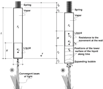
Consider the scheme of Fig. 1.
Figure 1. The container used to generate the mathematical model. a) Before the bubble generation, b) after the bubble generation.
Any heat source can be used, provided that liquid is heated and maintained close to the bottom of the container so that the “explosion” dislocates all the mass of the liquid. In the pictures of Figs. 3 and 5, a candle flame was used.
When the liquid moves upwards, the container moves downwards. In this item, the main objective was to quantify the movement of the container, which, as mentioned, is coupled to the movement of the liquid. The internal and the external forces acting on the container were considered.
Considering first the inner side, Fig. 1a shows that the pressure on the bottom of the cylinder, resulting from the pressure of the gaseous phase above the liquid, ps, and the liquid weight, Wl, is ptotal
= Wl/A+ps, where A is the transversal area of the container. A bubble
is formed between the liquid and the bottom of the container only if its pressure pb is higher than ptotal, that is pb > Wl/A+ps. It may be expressed as:
p s l
b p E
D W
p + +
π
= 4 2 (1)
Ep is called here the “excess of pressure” which allows the bubble
to push the liquid upwards, and D is the diameter of the container. The resultant of forces applied on the liquid is then given by:
(
)
H D D E W H D D p p R p l s b liq π τ + π − = + + π τ + π − − = 0 2 0 2 44 (2)
where is the shear stress between the container and the liquid. Equation (1) shows that Ep is negative for small pb, a situation that occurs during cavity events. The subscript “liq” refers to the liquid.
Considering now the internal forces acting on the container: from Fig. 1(a), for the liquid at rest, only Wl contributes to the
resultant force in the inner side, because ps equally acts on the upper and the lower surfaces, resulting in a total null contribution. In Fig. 1(b), for the moving liquid, the resultant force on the inner side of the container is given by
(
)
π τ − π + = = π τ − π − = DH D Ep W DH D p p R l s b inner 0 2 0 2 4 4 (3)The “external” forces acting on the container are the weight of the container, Wc, the force of the spring, and the sum of the resistance forces, represented by FR. The resultant is:
(
)
Rc
outer W K y y F
R m
2 0+
−
= (4)
where K is the constant of the spring, y0 is the initial displacement of the spring (system at rest), and y2 is the additional displacement induced by the cavity. The sign of FR changes for upwards and
downwards movements. The resultant force on the container is the sum of Eqs. (3) and (4), that is:
(
)
R p l c con F DH D E y y K W W R m π τ − π + + + − + = 0 2 2 0 4 (5)The subscript “con” refers to the container. Figure 1(a) represents the system at rest, where the balance of forces is given by:
0
0=
−
+W Ky
Wc l (6)
In Fig. 1(b) the mass of liquid has upwards velocity Vl. (relative to
the observer) during the expansion of the cavity. Through action and reaction, momentum is transmitted to the bottom of the container. In other words, when a cavity pushes the liquid upwards, the container moves downwards, stretching the spring. The work done by the spring is given by the product of the force on the spring and the velocity of the container, Vc (relative to the observer), named here as “usable work”. Equations (2), (5), and (6) generate a set of two equations to calculate the movement of the cylinder, in the form:
π τ + π − = π τ − π + − = H D D E t d V d m F DH D E y K dt V d m p l liq R p c con 0 2 0 2 2 4 4 m (7)
Equations (7) are coupled through the shear stress τ0 and the
excess of pressure Ep. Hypothesis may be made for τ0, Ep, and FR, in
order to simplify the description of the movement. In the simplest case, if these variables are null, or constant, or functions only of time, Eqs. (7) are independent linear second order differential equations for y1 and y2. Resistance forces in oscillatory problems are usually assumed as proportional to the velocity (see, for example, Bronson and Costa, 2006). Following this assumption, τ0 = α (Vl +
Vc), and FR = ady2/dt, where α and a are proportionality constants.
Equations (7) are then transformed to:
π + α + π − = − − π + α − π + + − = H D t d y d t d y d D E t d y d m dt dy a DH t d y d t d y d D E y K dt y d m p liq p con 2 1 2 2 1 2 2 2 1 2 2 2 2 2 4
4 (8)
Note that Ep = 0 for times greater than the life time of the cavity, so that different solutions may describe the movement with and without the cavity. From Eq. (8), a third order equation for y2 results
for the movement of the container, given by:
(
)
t d dE m D y m m DH K dt dy m m aDH m K t d y d m DH m DH a dt y d p con liq con liq con con liq con 4 2 2 2 2 2 2 3 2 3 π = απ + + απ + + + απ + απ + + (9)The linearity of Eq. (9) depends on the relationship between Ep
time, Eq. (9) is linear and allows simpler comparisons between predicted and observed movements. This characteristic is explored here to compare calculated results and experimental data. Of course, different resistance laws lead to different governing equations. In the sequence, a solution for α = a = 0 and polynomial variations of
Ep with time is compared with the experimental results obtained
here.
Experimental Arrangements
The container
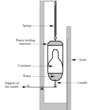
The container was built using a mercury lamp made of glass, having the dimensions shown in Fig. 2. The diameter of the container varies, implying also in slight horizontal movements of the liquid while it moves vertically. Because these horizontal movements had small effect on the vertical movement of the container, this form was considered adequate. The external metal contacts of the lamp were carefully removed. The orifice existing on the top of the lamp allowed to clean the white coating of the inner surface, and to fill the lamp with water. The internal metal contacts were maintained because the vertical movements may still be observed, although they of course introduced perturbations in the flow of the liquid.
Figure 2. Dimensions of the container used in the present experiments, built using a mercury lamp. Dimensions in mm.
The lamp was filled with water until the position of the orifice shown in Fig. 2. A mass of sand (quartz) of about 2 mg was added to the water. The sand added to the water avoids the formation of strong thermal convection, so that the heated water stays in contact with the bottom of the container. The water was then boiled during a period of about 5 hours, so that approximately 50% of it evaporated through the orifice. At this time, the internal atmosphere above the water was mainly composed by water vapor. With the water still boiling, the orifice was closed of melting the glass. The boiling was then stopped and the container was let to cool naturally, so that the internal pressure lowered continuously until the equilibrium condition for the environmental temperature was reached.
Different visualizations related to critical pressure and temperature may be conducted in such closed containers. In the present study the interest was directed to the generation of large scale cavities, intending to obtain large scale movements and usable work.
The mass of the container was 157.8 g, and the mass of the water was 680.4 g. The structure necessary to hold the container was built by conveniently cutting a plastic bottle, which was then attached to a spring, as shown in the sketch of Fig. 3. The total mass
of the spring and the holding structure was 130.0 g. The constant of the spring was K = 19.92 N/m.
Movement visualizations
The methodology followed to quantify the movement of the container may be so described: 1) the movement was recorded using a high velocity camera; 2) the films were analyzed in slow motion, and the frames containing the relevant information were selected; 3) distances were measured digitally on the selected frames; 4) graphs showing the movement along time were plotted; and 5) simultaneous phenomena occurring during the cavity events were selected for a more complete description of the experiments.
Figure 3 shows that the cavities were generated by increasing the local temperature at the bottom of the container, for which a candle was positioned below the container using a proper support. As mentioned, these cavities may then be called “ebullition events”. When the local temperature reaches the limit of the vapor pressure for the conditions in the container, a cavity is formed. Figures 4(a) through 4(l) show the evolution of a cavity for the container fixed to a support. A gas flame was used. The maximum expansion was attained at a time of 29.6 ms.
Figure 3. The experimental arrangement showing the container, the holding structure and the energy source. In this case a candle flame is shown.
Figure 4. Cavity at different moments. a) 0.0 ms, b) 8.0 ms, c) 16 ms, d) 24 ms, e) 32 ms, f) 40 ms, g) 48 ms, h) 56 ms, i) 64 ms, j) 76 ms, k) 88 ms, l) 128 ms. The velocity of the camera was 1250 fps.
Figure 5. Vertical movement of the container during a cavity event until the maximum amplitude was reached. A scale was added to the upper-right part of each picture. The container moves away from the equilibrium position (at rest) during the formation of the cavity. The velocity of the camera was 500 fps.
Figure 6. Mean amplitude of the movements of the container (y2 of Fig. 1)
along time (full line). The error bars consider the standard error for each point. The velocity of the camera was 500 fps.
Film propagation or film climbing effect
During the second half-time of the bubbles expansion a water film was formed at the wall of the container, which propagated upwards even when the water decelerated and inverted its movement. The film “climbed up” the wall until the upper end of the lamp, and fell back after the implosion of the cavity. The accumulation of water close to the wall, and the film formation may have different causes, two of which were considered here: 1) the horizontal movement of the water, induced by the curvature of the container, as sketched in Fig. 7(a). In this case, the quick horizontal dislocation of volumes of water induces, through mass conservation, a vertical distribution along the wall. The vertical propagation of the accumulated water is inertial. This “mechanism” was called briefly “dislocation effect”; 2) the second possible cause is a difference between the vertical and horizontal mass transports due to deceleration (Fig. 7(b)). The rotational movement of the water close to the wall may result in accumulation of water if the vertical deceleration does not imply in an immediate horizontal deceleration.
(a)
(b)
Figure 7. a) accumulation of water due to the curvature of the container, b) accumulation of water due to lateral movements induced by the relative velocity between wall and water .
Figures 8(a) to (g) show that the film forms where the walls converge (dislocation), and propagates upwards even in the neck of the lamp, where the wall is vertical and no accumulation occurs. As water continuously reaches the lower part of the neck, it must propagate, but the mean direction of the flow could imply in separation from the wall. Thus, interfacial conditions between glass and water seem to prevail, which may also involve the rotational movement within the film, maintaining it adhered to the surface (see detail in Fig. 8(g). Figure 8 was obtained using a fixed container. The film can also be observed in Fig. 5 (h to l) for a moving container.
Quick growing of bubbles at the surface of the water
during the upwards movement of the water, when perturbations allowed to incorporate air into the liquid (Fig. 8). Perturbations occurred along the wires (Fig. 8) and also at the surface, without touching the wires, showing that different causes may generate these bubbles. The quick growing of the bubbles while the water moved downwards was probably due to the high pressure difference between the upper atmosphere and the cavity.
Figure 8. Propagation of the water film “climbing” the wall. The arrows indicate the position of the film. The detail (g) of figure (f) shows the film still adhered to the wall in the neck of the lamp.
Figure 9. Macro cavity collapsing and showing the known central jet (dark color) and the “torus-like cavity” (light color) (1250 fps – each fifth frame is reproduced).
General implosion characteristics
The large size of the phenomenon, recorded at a camera speed of 1250 fps, allowed to easily observe the collapsing details. Figure 9 shows the breakdown of the “ceiling” of the bubble, which formed a central macro scale jet that crashed against the bottom of the container. These pictures were obtained for a fixed container, and
the observed movement was reproduced in all experiments (also see, for example, Fig. 4(f through j)). The formation of the central jet and the implosion of the bubble occur during the decreasing part of the graph of Fig. 6. The characteristics of the implosion are similar to the central microjets and the “torus like cavities” described for small bubbles by Shima (1996).
Force measurements
Moving container
The force done to move the container was obtained by multiplying the second derivative of y2 along time (d2y2/dt2) by the mass of the container and its holding structure (157.8 g + 130.0 g). The total time interval considered here was 0 < t < 70 ms. The second derivative was calculated using the dislocation and time data of each experiment, and the following five points approximation:
2 2 2
2
2 2 2
2 2 2
8
) 2 ( ) ( 4 ) ( 10
8
) ( 4 ) 2 (
t
t t y t t y t y
t
t t y t t y t d
y d
∆
∆ + + ∆ + + −
+
+ ∆
∆ − + ∆ − =
(10)
Five points were used to avoid too strong oscillations between calculated values at neighboring points. Figure 10 shows the mean values obtained for the force as a function of the time, together with the error bars of each point. Although somewhat sparse, the cloud of points allows to observe the following general characteristics:
•The maximum peak of force occurred at a time of around 5 ms.
•The minimum peak of force occurred at a time of around 25 ms. This time also corresponds to the maximum amplitude of y2, as
shown in Fig. 6.
Figure 10. Force against time for the moving container. Results obtained calculating d2y2/dt
2
with Eq. (10) and using a mass of 287.8 g. The solid lines are adjusted low order functions (11a and b), representing the mean behavior.
Figure 10 also shows solid lines, which correspond to two adjusted low order polynomial functions, mathematically expressed as:
(
)
s t
for t
t F
b
s t
for t F
a
070 . 0 025 . 0 035
. 0
025 . 0 05 . 3
035 . 0
025 . 0 05 . 4 1 * 9338 . 95 )
025 . 0 0 59
. 7702 6311 . 96 )
2
< <
−
+
+
− −
− =
< < −
=
(11)
the present purposes. Equations (11) were used as first approximations in the theoretical analysis, in which the use of low order polynomials of t representing Ep were tested in the calculations of y.
Fixed container
A second set of experiments was conducted to measure the force on the container without movement, for which it was fixed to a charge cell of 500 N. Three experiments were performed, and the results are shown in Fig. 11. Some general characteristics can be described:
• The maximum peak occurred at a time of around 2.9 ms.
• The minimum peak occurred at a time of around 31 ms.
• High frequency oscillations were observed, probably caused by the natural frequency of the charge cell.
Figure 11. Evolution with time of the force applied on the container. Data obtained using a 500 N charge cell.
The maximum measured peak of force was 476 N, while the minimum peak was −136 N. The high frequency oscillations, if due to resonance of the charge cell, may imply in a real peak lower than the measured value. A straight line was adjusted to the data for 10 <
t < 20 ms, furnishing F = 186.156-10651.6t. In Fig. 11 this line is extrapolated to allow visual comparisons between the linear behavior and the response of the charge cell. The minimum peak of the force and maximum expansion of the cavity occurred at very similar times (both around 30 ms). Figure 10 was obtained using the mass of the container and its holding structure, while in Fig. 11 the force is due to the acceleration of the mass of liquid.
Comparisons Between Measured y2 and Model Calculations Using Time Evolutions for Ep
As already commented, Eq. (9) was linearized here considering
α= a = 0 and polynomial variations of Ep with time, as shown in the
sketch of Fig. 12. In the present item, calculated positions of the container are compared with the mean measured positions.
Figure 12. Simplified evolution of Ep used in Eq. (9), following the force
measurements of Fig. 10.
Equation (9) may be integrated once, furnishing:
con p con m E D y m K dt y d 4 2 2 2 2 2 π =
+ or
p con E D y K dt y d m 4 2 2 2 2 2 π =
+ (12)
Figure 6 shows that following boundary conditions may be used:
end T t for dt y d and y iii or T t for dt y d and y y ii or t for dt y d and y i = = = = = = = = = 0 0 ) ( 0 ) ( 0 0 0 ) ( 2 2 2 max 2 2 2 (13)
For the present data, ymax~35 mm, T~25 ms, and Tend~70 ms. Ep
was not measured, but it was evaluated, as a first approximation, by dividing equations (11a, b) by the constant horizontal area of the container (Ep = 4F/πD2). This is an approximation, because to obtain Ep it would be necessary to consider F, Ky2, and the resistance forces; and because the horizontal area exposed to Ep
varies during the experiment (due to the form of the container). The low order polynomials for Ep were used here in the more complete
Eq. (12) (that is, including Ky2) to verify if viable theoretical solutions of y2 are obtained with the suggested simplifications. Equations (11a,b) and (12) led to the solution:
− + + − = t m K t m K t y con con gro cos 85096 . 4 sin 4781 . 46 677 . 386 85096 . 4 2
(
)
480 . 346 cos 629 . 341 sin 9839 . 66 035 . 0 025 . 0 05 . 3 035 . 0 025 . 0 05 . 4 1 81596 . 4 2 2 + − − − − + − − − = t m K t m K t t y con con dec (14)The subscripts “gro” and “dec” refer to the growing and the decreasing segments of y2, respectively. Contours (13i) were used
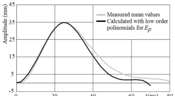
for the growing segment and contours (13ii) were used for the decreasing segment. The results are presented in Fig. 13, where the black solid line represents Eqs. (14), while the gray line shows the mean observed behavior. As can be seen, the calculated behavior in the interval 0 < t < 70 ms follows the general shape of the measured curves, although the proximity between calculated and observed mean values is better for the interval 0 < t < 30 than for the interval 30 < t < 70 ms.
Figure 13. Calculated (black) and mean value of the measured (gray) displacements of the container, considering low order polynomials for Ep.
Conclusions
It was shown that macro-scale cavities generate usable work while moving the container of the fluid in which the cavities are produced. In this study, a movement similar to a piston was induced by controlling the starting-position of the cavity, and the usable work was represented by the stretching of a spring.
To experimentally verify the generation of movements and forces, a glass container was built and adequately filled with water, which was maintained at low pressure. As mentioned, the container was fixed to a spring, and the cavities were formed by heating the bottom of the container. These cavities were thus understood as ebullition events. The water was heated in the vicinity of the central region of the bottom, and its convection was hindered by concentrating a small amount of sand in the heated region.
The cavities were formed when the temperature of the water at the bottom of the container reached the vapor condition. The maximum diameter of the cavities followed the diameter of the container (117 mm). The forces generated by the expansion of the cavity pushed the water upwards and the container downwards. The force applied to the container stretched the spring to which it was fixed, thus producing work. The experimental arrangements allowed to obtain displacements of the container with peak values in the range of 33 to 41 mm, for elapsed times around 25 to 28 ms. The experiments were recorded using a high speed camera, at a rate of 500 frames per second, generating sets of values of time and displacement for each experiment. These data were used to calculate the acceleration of the container along time, and the force acting on it. The results allowed to approximately express the force as a function of time using low order polynomials. For growing displacements, a first order polynomial was used for the force, while for decreasing displacements; a second order polynomial was used for the force.
Considering the theoretical propositions, a third order, nonlinear, one-dimensional governing differential equation was proposed for the movement of the container. The equation was further linearized representing Ep by polynomials of time, allowing to obtain a theoretical solution, in which resistance forces were neglected. The theoretical positions of the container were compared with the measured mean values, showing that the present formulation allows to reproduce the observed phenomena. Further, the results may suggest that a more complete prediction must consider the resistance laws and the dependence between Ep and the volume occupied by the cavitation (represented, in the formulation, by the sum y1 + y2).
Thus, the present study allowed: a) to generate and observe scale cavities in a liquid, b) to generate and observe macro-scale movements of the container that contains the liquid, c) to obtain the value of the force transmitted to the container during ebullition events, d) to verify that the theoretical equation allows calculations that follow the general form of the observed
movements, and e) to propose further uses of the equation considering resistance effects and improved approximations for Ep.
Additional characteristics related to the quick movement of the liquid were also observed and described: a) the film propagation along the internal surface of the container, mainly associated with the lateral dislocation of the water; b) the quick growing of bubbles at the surface of the liquid, mainly associated with disturbances at the water surface; and c) the collapsing of the macro cavities, showing a behavior similar to that described for small cavities in liquids.
Acknowledgements
The authors thank CAPES, FAPESP, and CNPq, for the support of this research line, and to Prof. Gerhard Ribatski, for the help to obtain the images used in this study.
References
Alehossein, H. and Qin, Z., 2007, “Numerical analyisis of Rayleigh-Plesset equation for cavitating jets”, Int. Journal for Numerical Methods in Engineering, Vol. 72, pp.780-807.
Almeida, W.J., 2007, “Structural optimization of FDM prototypes based on finite elements analysis (Otimização estrutural de protótipos fabricados pela tecnologia FDM utilizando o método dos elementos finitos”, MSc. Thesis, School of Engg. at São Carlos, University of São Paulo, Brazil, 110 p. (in Portuguese).
Assis, M.P., Dalfré Filho, J.G. and Genovez, A.I.B., 2008, “Cavitating jet devices for water disinfection (Equipamento tipo jato cavitante para a desinfecção de água”, XVII Brazilian Simposium on Water Resources, (in Portuguese).
Azuma, Y., Kato, H., Usami, R. and Fukushima, T., 2007, “Bacterial sterilization using cavitating jet”, Journal of Fluid Science and Technology, Vol. 2, No.1, pp. 270-281.
Brenner, M.P., Hilgenfeldt, S. and Detlef, L., 2002, “Single bubble sonoluminescence”, Reviews of Modern Physics (The American Physical Society), Vol. 74, No. 2, pp. 425-484.
Bronson, R. and Costa, G., 2006, “Differential Equations”, Schaum’s Outline Series, 3rd Edition, McGraw Hill, 385p.
d’Agostino, L. and Salvetti, M.V. (eds.), 2007, “Fluid dynamics of cavitation and cavitating turbopumps”, International Centre for Mechanical Sciences, CISM Courses and Lectures, Vol. 496, Springer Wien New York.
Falvey, H.T., 1990, “Cavitation in chutes and spillways”. 1st ed. Denver: United States Bureau of Reclamation, 145 p.
Gaitan, D.F., Crum, L.A., Roy, R.A. and Church, C.C., 1992, “Sonoluminescence and bubble dynamics for a single, stable, cavitation bubble”, The Journal of the Acoustical Society of America, Vol. 91, No. 6, pp. 3166-3183.
Kodama, T. and Tomita, Y., 2000, “Cavitation bubble behavior and bubble-shock wave interaction near a gelatin surface as a study of in vivo bubble dynamics”, Appl. Phys. B, Vol. 70, pp. 139-149.
Leighton, T.G., 2007, “Derivation of the Rayleigh-Plesset equation in terms of volume”, ISVR Technical Report No. 308, University of Southampton, Institute of Sound & Vibration Research, 17 p.
Lohse, D., Schmitz, B. and Versluis, M., 2001, “Snapping shrimp make flashing bubbles”, Nature, Vol. 413, pp. 477-478.
Patek, S.N. and Cladwell, R.L., 2005, “Extreme impact and cavitation forces of a biological hammer: strike forces of the peacock mantis shrimp Odontodactylus scyllarus”, The Journal of Experimental Biology, Vol. 308, pp. 3655-3664.
Sánchez, R., Juana, L., Laguna, F.V. and Rodriguez-Sinobas, L., 2008, “Estimation of cavitation limits from local head loss coefficient”, Journal of Fluids Engineering, October, Vol. 130, 9 p.
Shima, A., 1996, “Studies on bubble dynamics”, Shock Waves, Vol. 7, pp. 33-42.
Tomita, Y., Tsubota, M. and An-naka, N., 2001, “Energy Evaluation of shock wave emission and bubble generation by laser focusing in liquid nitrogen”, International Symposium on Cavitation CAV 2001, session A2.006, 8 p.
Upcraft, S. and Fletcher, R., 2003, “The rapid prototyping technologies”, Assembly Automation, Vol. 23, No. 4, pp. 318-330.
Versluis, M., Schmitz, B., von der Heydt, A. and Lohse, D, 2000, “How snapping shrimp snap: through cavitating bubbles”, Science, Vol. 289, pp. 2114-2117.