Abstract—This article deals with the forecasting of interval and triangular fuzzy number series based on accumulation method GM (1, 1) (AMGM (1, 1)) and Markov chain. Because AMGM (1, 1) only suit precise number, the interval and triangular fuzzy number series are transformed into precise number series. The transformation process maintains the integrity and the relative position of the boundary points of the fuzzy number. Because GM (1, 1) is not suitable for the long-term and strongly fluctuating prediction, Markov chain theory is applied to modify AMGM (1, 1). The interval predictions of the Consumer Price Index and the power load show the effectiveness of the models proposed in the paper.
Index Terms—fuzzy number, grey model, accumulation method, Markov chain
I. INTRODUCTION
HE traditional prediction models, such as the autoregressive moving-average model, the bilinear model and the nonlinear autoregressive model, are only suitable for the precise number series. In many applications, such as the electric power load, the prices of oil, stock, or gold, the daily air temperature, and the exchange rate, the observed data fluctuate at any time. Then using interval fuzzy numbers to represent these data is more reasonable than using precise data. In [1], Zadeh introduced fuzzy number firstly, and fuzzy mathematics has been applied to many fields [2]. The common types of interval fuzzy numbers are binary interval fuzzy number, triangular fuzzy number (or trinary interval fuzzy number) and trapezoidal fuzzy number. In this article, we consider the forecasting of interval and triangular fuzzy number series.
Another problem with the traditional prediction approaches is that they require a large corpus of data because these predictors are constructed on the assumption about the distribution of the population [3-5]. It is difficult to confirm
Manuscript received December 21, 2015; revised June 10, 2016. This work was funded by the Science and Technology Research Projects of Guangxi Colleges (Grant No. KY2015YB113), the National Science Foundation of China (Grant No. 71561008), Guangxi District Natural Science Fund of China (Grant No. 2014GXNSFAA118003 and 2014GXNSFAA118010), the Natural Science Foundation Project of CQ CSTC (Grant No. cstc2014jcyjA00054), and the Fundamental Research Funds for Chongqing Education Commission (Grant No. KJ1501113).
X. Y. Zeng is with the School of Mathematics and Computational Science, Guilin University of Electronic Technology, Guilin, China (e-mail: zengxyhbyc@ 163.com).
L. Shu is with the School of Mathematical Science, University of Electronic Science and Technology of China, Chengdu, China (e-mail: shul@uestc.edu.cn)
J. Jiang is with Chongqing University of Arts and Sciences, Chongqing, China.
the population distribution with small sample. For this problem, Deng proposed grey models focusing on uncertainty characterized by poor information and a small sample [6, 7]. GM (1, 1) is one of the basic grey models. It can be built on the basis of at least four data points and has good precision [8-12]. However, just as many other forecast methods, grey models are only applicable to precise numbers. In the modeling process of GM (1, 1), some calculations about the fuzzy numbers, such as accumulated generating operation, inverse accumulated generating operation, and matrix multiplication and inversion cannot be achieved. Therefore, the classical modeling process is not suitable for the fuzzy number series. In the paper, the interval fuzzy sequence is transformed into real series. First, GM (1, 1) models are built on these precise series, and then, through the restoration process, the predicted values of the interval fuzzy number series are obtained.
The prediction curve of GM (1, 1) can only reflect the integral development tendency of the series. Thus it only suits the series with weak fluctuation [13-15]. For the fluctuating series, GM (1, 1) should be modified. In [16], the Markov chain forecasting model is combined with GM (1, 1), and the combined model has good effect on the fluctuating real series. In this paper, the prediction results of GM (1, 1) model will be further modified via the Markov-chain forecasting model when the fuzzy series has strongly fluctuation.
The rest of the article is organized as follows. In Section 2, we provide the parameter estimators based on accumulation method (AM) and prove some of its properties. In Section 3, the transformation processes of the interval and triangular fuzzy number series are provided. The modeling process of the accumulated method GM (1, 1) (AMGM (1, 1)) is provided in Section 4. In section 5, the modified process via Markov chain prediction model is proposed. In Section 6, two applicable examples are given to illustrate the effectiveness of the model proposed in the paper. Finally, conclusions are discussed in Section 7.
II. BASIC THEORY OF ACCUMULATION METHOD
The accumulation method (AM) was first introduced by Italian mathematician, P. Marchsi, in 1778. It is a new method of the parameter estimation and has been applied to many fields. In [17], Zeng and Xiao introduced the AM method into GM (1, 1) and analyzed its morbidity problem. They concluded that the condition number of the AM method is less than the least square method.
Let
X
{
x
(
1
),
x
(
2
),
,
x
(
n
)}
be an original series. Then each-order accumulation sum is defined as,Fuzzy Time Series Forecasting based on Grey
Model and Markov Chain
Xiangyan Zeng, Lan Shu, Jing Jiang
(1)
1 1
( )
(1)
(2)
( )
( ),
n n
i i
x i
x
x
x n
x i
(2) 1 (1) 1 1( )
(1) ( (1)
(2))
( (1)
(2)
( ))
( ),
n
i
n i
i j
x i
x
x
x
x
x
x n
x j
and so on. Thus, each-order accumulation sum is defined as follows.
( ) ( 1)
1 1 1
( )
( )
n n i
r r
i i j
x i
x j
,r
1, 2,
, (1)where ( ) 1
1
n r
i
is called the r-order basic accumulation sum. Generally, the tedious calculation is not convenient for the practical application. In [18], Cao and Zhang have provided the following convenient formula for the accumulation sums.( ) 1
1
1 1
( )
( )
n n
r r
n i r
i i
x i
C
x i
1
1
(
1)(
2)
(
1) ( ),
(
1)!
n
i
n i
n i
n i
r
x i
r
(2) and ( ) 1 11
1
(
1)
(
1)
!
n
r r
n r i
C
n n
n
r
r
. (3)Next, give the process of parameter estimation using the AM method. Let
1 2
{ ( ),
x t x t
( )
,
x t y t
m( ), ( )}
,t
1, 2,
,
n
, be n groups of samples. Based on these samples, the parameters
i,i
1, 2,
,
m
, of the following linear model will be estimated.0 1 1
( )
( )
m m( )
( )
y t
x t
x t
t
, (4)where,
( )
t
is a stochastic disturbance with zero mean value. First, the accumulation sum is operated on both sides of (4). With 1+m parameters, the maximum order of the accumulation sum should be 1+m. Then, we getr r
Y
X
, (5)where,
(1) (2) ( 1)
1 1 1
( )
( )
( )
T
n n n
m r
t t t
Y
y t
y t
y t
,(1) (1) (1)
1
1 1 1
(2) (2) (2)
1
1 1 1
( 1) ( 1) ( 1)
1
1 1 1
1
( )
( )
1
( )
( )
1
( )
( )
n n n
m
t t t
n n n
m
t t t
r
n n n
m m m
m
t t t
x t
x t
x t
x t
X
x t
x t
, 0 1 m
, and(1) 1 (2) 1 ( 1) 1
( )
( )
( )
n t n t n m tt
t
t
.Thus, the parameters are estimated as, 1
ˆ
r r
X
Y
. (6)
It can be easily shown that
ˆ
is the linear unbiased minimum variance estimation of
,. From (6), we can see that AM is based directly on the samples, which avoids the assumptions about the error. Next, we give the geometric meaning of the AM method based on the theory of the center of gravity.Assume that each data of
X
{ (1), (2),
x
x
, ( )}
x n
represents a point of the number axis. The center of gravity of one point is the point itself:
x
x
(1)
. The center of gravity of two points (x
(1)
andx
(2)
) is(1)
(2)
2
x
x
x
.The center of gravity of three points (
x
(1)
,x
(2)
andx
(3)
) divides the segment between(1)
(2)
2
x
x
and
x
(3)
into 1 : 2, namely,1
(1)
(2)
1
(2
(3))
( (1)
(2)
(3)),
3
2
3
x
x
x
x
x
x
x
and so on, the center of gravity of
X
{ (1), (2),
x
x
, ( )}
x n
is1
( )
1
( (1)
(2)
( ))
n
i
x i
x
x
x
x n
n
n
From (2) and (3), we have (1)
1 1
( )
( )
n n
i i
x i
x i
and(1) 1
1
n
i
n
. (1) (1)1 1
( )
1
n n
i i
x i
is called the first-order center operator.Normally, the center of gravity of
(
m
n
)
points divides the segment between the center of gravity of the topm
points and the center of gravity of the lattern
points inton m
:
. Thus, the center of gravity of the following data:(1)
x
,(1)
(2)
2
x
x
,
(1)
(2)
(3)
3
x
x
x
,
, 1( )
n
i
x i
n
,
is
(2)
1 1
(2) 1
(1) ( (1)
(2))
( )
( )
1 2
1
n n
i i
n
i
x
x
x
x i
x i
x
n
,which is called the 2-order center operator. And so on,
( ) ( )
1 1
( )
1
n n
r r
i i
x i
is called ther
-order center operator. From the above analysis, we know that the geometric meaning of AM is for a gravity-center line based on the known sample points. Moreover, the method of AM achieves the data smoothing at most. Thus, the conservatism is enhanced and the ill effects of outliers are weakened.III. TRANSFORMATION OF THE FUZZY NUMBER SERIES
The forecasting models can be built on the boundaries of the fuzzy number directly. This idea, however, will result in the broken integrity of the fuzzy numbers and the relative positions of the disordered boundaries of the interval fuzzy number in the forecasting results. Therefore, we consider transforming the interval fuzzy number first, and then using the transformed series to build the forecasting model.
A. Transformation of Interval Fuzzy Number Series
Let
X
~
{
~
x
(
1
),
~
x
(
2
),
,
~
x
(
n
)}
be the interval fuzzy sequence, where,x i
( )
[
x i x i
L( ),
U( )]
. Herex i
L( )
and( )
Ux i
are the lower and upper boundaries, respectively. The mid-point and the length of the interval number respectively are( )
( )
( )
2
L U
x i
x i
m i
, (7)and
( )
U( )
L( )
l i
x i
x i
. (8)Let the mid-point sequence (
M
) and the length sequence (L
) respectively be)}
(
,
),
2
(
),
1
(
{
m
m
m
n
M
,)}
(
,
),
2
(
),
1
(
{
l
l
l
n
L
.And now, transform the interval fuzzy sequence into two precise sequences as,
)}
(
~
,
),
2
(
~
),
1
(
~
{
~
n
x
x
x
X
{ (1), (2),
, ( )}
{ (1), (2),
, ( )}
M
m
m
m n
L
l
l
l n
The bounds of the interval fuzzy number can be restored respectively as,
( )
( )
( )
2
L
l i
x i
m i
, and( )
( )
( )
2
U
l i
x i
m i
. (9)Obviously,
x i
L( )
x i
U( )
, which ensures the relative positions of the bounds of the interval number in the forecasting results.B. Transformation of Triangular Fuzzy Number Series
Let the triangular fuzzy sequence be
)}
(
~
,
),
2
(
~
),
1
(
~
{
~
n
x
x
x
X
,where,
( )
[
L( ),
M( ),
U( )]
x i
x i x
i x i
,i
1, 2,
,
n
. The gravity center of the fuzzy number or the mean value serves as the index of the comparison and sort order of the fuzzy number. For the triangular fuzzy number, the gravity center is calculated as,( )
( )
( )
( )
3
L M R
x i
x
i
x i
f i
. (10)The lengths between the three bounds are calculated as,
( )
M( )
L( )
p i
x
i
x i
andq i
( )
x i
U( )
x
M( )
i
. (11)Let the gravity center sequence (
F
) and the tow length sequences (P
andQ
) respectively be{ (1), (2),
, ( )}
F
f
f
f n
,{ (1), (2),
, ( )}
P
p
p
p n
,{ (1), (2),
, ( )}
Q
q
q
q n
,)}
(
~
,
),
2
(
~
),
1
(
~
{
~
n
x
x
x
X
{ (1), (2),
, ( )}
{ (1), (2),
, ( )}
{ (1), (2),
, ( )}
F
f
f
f n
P
p
p
p n
Q
q
q
q n
The reduction process is given by
2 ( )
( )
( )
( )
3
3
L
p i
q i
x i
f i
,( )
( )
( )
( )
3
3
M
p i
q i
x
i
f i
, (12)( )
2 ( )
( )
( )
3
3
U
p i
q i
x i
f i
.Obviously,
x i
L( )
x
M( )
i
x i
U( )
, which ensures the relative positions of them in the forecasting results.From (7), (8), (10), and (11), the new transformed series are simultaneously affected by the bounds of the fuzzy number and, actually, they are the weighted mean values of the bounds. These characteristics maintain the integrity of the fuzzy number and weaken the jumping degree of the boundaries. Thus, the smoothness of the transformed series is better than the raw boundary series. In addition, the reduction processes, (9) and (12), ensure the relative positions of the boundaries of interval numbers are not disordered in the prediction.
IV. PREDICTION PROCESS BASED ON AMGM(1,1) The accumulation method GM (1, 1) (AMGM (1, 1)) is built using the transformed series, and then through the reduction process, the predicted values of the fuzzy numbers are obtained. First, the modeling process for the mid-point series
M
{
m
(
1
),
m
(
2
),
,
m
(
n
)}
is given as follows. The grey differential equations of GM (1, 1) based on M are(1)
( )
M( )
Mm i
a z
i
,i
1, 2,
,
n
, (13) where(1) (1) (1)
( )
0.5(
( )
(
1))
z
i
m
i
m
i
,2, 3,
,
i
n
, (14) and(1)
( )
m
i
1
(1)
(2)
( )
( )
i
j
m
m
m i
m j
,1, 2,
,
i
n
. (15) First, the accumulation sum is operated on both sides of (13). Assume that the highest order of the accumulation sum is denoted byr
. Because (13) has tow parameters, it is certain thatr
2
.(1) (1) (1) (1)
2 2 2
( )
( )
1
n n n
M M
i i i
m i
a
z
i
,(2) (2) (1) (2)
2 2 2
( )
( )
1
n n n
M M
i i i
m i
a
z
i
. (16)Using the results in [18] described earlier, we have the calculation formulas of the following accumulation sums.
(1) (1) (1)
2 2
( )
( )
n n
i i
z
i
z
i
, (1)2 2
( )
( )
n n
i i
m i
m i
(2) (1) 1 (1) (1)
1
2 2 2
( )
( )
(
1)
( )
n n n
n i
i i i
z
i
C
z
i
n i
z
i
,(2) 1
1
2 2 2
( )
( )
(
1) ( )
n n n
n i
i i i
m i
C
m i
n i
m i
,(1) 1
2
1
1
1
n n i
C
n
, (2) 2 2 1 2(
1)
(
1)
1
2
2
n
n i
n n
n n
C
n
n
.Let
(1) (1) (1)
2 2
(2) (1) (2)
2 2
( )
1
( )
1
n n
i i
r n n
i i
z
i
X
z
i
, (1) 2 (2) 2( )
( )
n i r n im i
Y
m i
, and M Ma
A
.Then the matrix form of (16) can be expressed as,
r r
A
Y
X
, (17) and the parameter estimator is obtained as,1
ˆ
ˆ
ˆ
M r r Ma
A
X
Y
. (18)From (13), the predictive formula is deduced as follows. Due to
z
(1)( )
i
0.5(
m
(1)( )
i
m
(1)(
i
1))
, (13) is transformed as,(1) (1)
( )
(
( )
(
1))
2
M
M
a
m i
m
i
m
i
.From (15), we have
(1)
( )
( ( )
2
(
1))
2
M
M
a
Then,
(1)
(
1)
( )
1 0.5
M M
M
a
m
i
m i
a
.From (15),
m
(1)(
i
1)
m
(1)(
i
2)
m i
(
1)
, so(1)
(
1)
( )
1 0.5
M M
M
a
m
i
m i
a
(1)
( (
1)
(
2))
1 0.5
M M
M
a
m i
m
i
a
(1)
(
2)
(
1)
1 0.5
1 0.5
M M M
M M
a
m
i
a
m i
a
a
(
1)
(
1)
1 0.5
M
M
a
m i
m i
a
2
(
1)
2
M
M
a
m i
a
2
2
(2)
2
i M
M
a
m
a
2
2
(1)
2
1 0.5
i
M M M
M M
a
a
m
a
a
2
1
2(2
)
(
(1))
(2
)
i
M M M
i M
a
a
m
a
. (19)After the estimator is obtained from (18), and
m
(1)
is adopted as the starting value, (19) can be used as the prediction formula. Namely, the predicted values ofm i
( )
is2
1
ˆ
ˆ
ˆ
2(2
)
(
(1))
ˆ
( )
ˆ
(2
)
i
M M M
i M
a
a
m
m i
a
,2, 3,
i
. (20) For the other transformed sequences (L
,F
,P
andQ
) AMGM (1, 1) can be established similarly. Finally, from (9) and (12), the predicted values of the boundary values of the fuzzy number can be achieved.V. MODIFIED PROCESS BASED ON MARKOV CHAIN
The prediction curve of GM (1, 1) is a smooth curve, which can reflect the general development trend of the raw series. The fluctuation rule of the series is not reflected. Therefore, for the strongly fluctuating series, the forecast precision of GM (1, 1) is not satisfactory. The Markov-chain forecasting can reflect the fluctuation rule of the series and can be used to modify the above proposed models.
For AMGM (1, 1) proposed in Section 4, the prediction series of the mid-point series
M
{
m
(
1
),
m
(
2
),
,
m
(
n
)}
is
M
ˆ
{ (1), (2),
m
ˆ
m
ˆ
, ( ),
m n
ˆ
}
. The modified process ofM
ˆ
is given as follows. For the other transformed sequences (L
,F
,P
andQ
) the modified process of their prediction series (L
ˆ
,F
ˆ
,P
ˆ
andQ
ˆ
) is similar asM
ˆ
.Step 1 Status partition
Based on the ratios
m i m i
( )
ˆ
( )
,i
1, 2,
,
n
, the system is divided intos
statuses,: [ ,
]
i i i
E
A B
,i
1, 2,
,
s
.Step 2 Establish the transition probability matrix
Let
N k
ij( )
be the number of raw data transferred from StatusE
i toE
j byk
steps. LetN
i be the occurrence number ofE
i. Then the transition probability fromE
itoj
E
byk
steps is( )
( )
ijij
i
N k
P k
N
,i j
,
1, 2,
,
s
. The transition probability matrix is11 12 1
21 22 2
1 2
( )
( )
( )
( )
( )
( )
( )
( )
( )
( )
s
s
s s ss
P k
P k
P k
P k
P k
P k
P k
P k
P k
P k
. (21)
Step 3 1-step predicted values identification If
m n m n
( )
ˆ
( )
is in the status ofE
h andmax
hj(1)
hl(1)
jP
P
,the modified values of
m n
ˆ
(
1)
is calculated as,1
ˆ
(
1)
(
1)
(
)
2
l lm n
m n
A
B
. (22)If
m n m n
( )
ˆ
( )
is in the status ofE
h andmax
hj(1)
jP
does not exist, the modified values ofm n
ˆ
(
1)
is taken as the expectation,1
1
ˆ
(
1)
(
1)
[
(1) (
)]
2
s
hj j j
j
m n
m n
P
A
B
. (23)Step 4 2-step predicted values identification If
m n m n
( )
ˆ
( )
is in the status ofE
h andmax
hj(2)
hl(2)
the modified values of
m n
ˆ
(
2)
is calculated as,1
ˆ
(
2)
(
2)
(
)
2
l lm n
m n
A
B
. (24)If
m n m n
( )
ˆ
( )
is in the status ofE
h andmax
hj(2)
jP
is not exist, the modified values ofm n
ˆ
(
2)
is the expectation,1
1
ˆ
(
2)
(
2)
[
(2) (
)]
2
s
hj j j
j
m n
m n
P
A
B
. (25)Similarly, the multi-step predicted values can be obtained.
VI. ILLUSTRATIVE EXAMPLES
Example 1 Small sample with weak fluctuation
The State Statistics Bureau of China provides Consumer Price Index (CPI) of each month (See China Statistical Yearbook). We take the mean value of twelve months of one year as the mid boundary of the triangular fuzzy number. The minimum and maximum of twelve months are taken as the lower and upper boundaries of the triangular fuzzy number, respectively. We take the records from 2002 to 2005 as the raw series to establish AMGM (1, 1) and the value in 2006 will be predicted. The raw data from 2002 to 2005 are given in TABLE I.
TABLE I
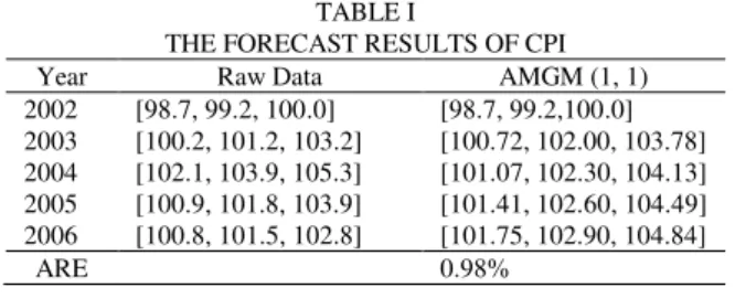
THE FORECAST RESULTS OF CPI Year Raw Data AMGM (1, 1) 2002 [98.7, 99.2, 100.0] [98.7, 99.2,100.0] 2003 [100.2, 101.2, 103.2] [100.72, 102.00, 103.78] 2004 [102.1, 103.9, 105.3] [101.07, 102.30, 104.13] 2005 [100.9, 101.8, 103.9] [101.41, 102.60, 104.49] 2006 [100.8, 101.5, 102.8] [101.75, 102.90, 104.84]
ARE 0.98%
First, due to the transformations (10) and (11), the three transformed series (
F
,P
andQ
) are obtained. AMGM (1, 1) is built usingF
,P
andQ
, respectively. The parameter estimates of AMGM (1, 1) by method of AM areF
:ˆ
0.0032
ˆ
101.6803
F
F
a
,P
:ˆ
0.0364
ˆ
1.3200
P
P
a
,Q
:ˆ
0.0290
ˆ
1.7314
Q
Q
a
.From (20), the predicted values of
F
,P
andQ
can be obtained. From restoration formula (12), the predicted series from 2002 to 2006 is calculated and are shown in Table 1. The results show that the average relative error (ARE) of AMGM (1, 1) is only 0.98%. In Fig. 1, the prediction curve is given and has good fitting effect. Although only four triangularfuzzy numbers are used, the precision is satisfactory. However, we can see that the fluctuation of the given series is weak. When the sample is large and has strong fluctuation, this example cannot illustrate the effectiveness of the proposed model.
2002 2002.5 2003 2003.5 2004 2004.5 2005 2005.5 2006 95
100 105 110 115 120
Year
B
o
u
n
d
a
ri
e
s
o
f
C
P
I
Raw Value AMGM(1,1)
Fig. 1. Raw values and results of AMGM(1,1) for CPI
Example 2 Large sample with strong fluctuation
Power load keeps changing and its forecasting is not suitable to be expressed as an exact number. Based on the real number series, [19] and [20] obtained the interval prediction by the degree of confidence or coverage probability. We have got the power load data of one district of Guilin City in China from September 1 to September 5, 2014. First, one day is divided into four time buckets: 00:00-06:00, 06:00-12:00, 12:00-18:00, and 18:00-24:00, which can represent four stages of the life of one day. The minimum value of power load in one time bucket is as the left boundary of the interval number, and the maximum value is as the right boundary. The raw interval series is shown in TABLE II.
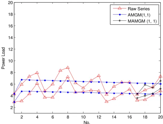
The prediction curves of AMGM (1, 1) are shown in Fig. 2. We can see that the integral development trend of the interval series is reflected, but the fluctuation rule is not shown. The average relative error (ARE) of the fitting values from September 1 to September 4 is 17.9%, and the average relative error (ARE) of the prediction values on September 5 is 22.24%. Therefore, the accuracy of AMGM (1, 1) is not satisfactory for the fluctuation series. Next, the results of AMGM (1, 1) will be modified via Markov chain forecasting method.
First, from (7) and (8), the transformed series (
M
andL
) of the raw series and the transformed series (M
ˆ
andL
ˆ
) of the forecasting series of AMGM (1, 1) are calculated respectively. The calculated values and the ratios (M M
/
ˆ
and
L L
/
ˆ
) are all shown in TABLE II. Step 1 Status partitionBased on the ratios
m i m i
( )
ˆ
( )
andl i
( )
l i
ˆ
( )
,i
1,
2,
,
n
, shown in TABLE II, the system is divided into four statuses shown in TABLE III.Step 2 Establish the transition probability matrix
From TABLE II, the 1-step transition probability matrix of
ˆ
/
TABLE II
THE TRANSFORMED SERIES AND THEIR RATIOS
No. Time
Raw Series AMGM(1,1) Ratio (%)
Raw values
M
L
M
ˆ
L
ˆ
M M
/
ˆ
L L
/
ˆ
1 9-1: 00:00-06:00 [2.9, 4.3] 3.60 1.4 3.6000 1.40002 9-1: 06:00-12:00 [3.1, 5.9] 4.50 2.8 5.7808 2.3965 77.84 116.84 3 9-1: 12:00-18:00 [4.3, 7.3] 5.80 3.0 5.7410 2.3143 101.03 129.63 4 9-1: 18:00-24:00 [6.1, 7.9] 7.00 1.8 5.7014 2.2350 122.78 80.54 5 9-2: 00:00-06:00 [3.7, 4.8] 4.25 1.1 5.6621 2.1584 75.06 50.96 6 9-2: 06:00-12:00 [3.7, 6.0] 4.85 2.3 5.6231 2.0845 86.25 110.34 7 9-2: 12:00-18:00 [5.4, 8.3] 6.85 2.9 5.5843 2.0130 122.67 144.06 8 9-2: 18:00-24:00 [7.2, 8.8] 8.00 1.6 5.5459 1.9440 144.25 82.30 9 9-3: 00:00-06:00 [4.6, 6.2] 5.40 1.6 5.5076 1.8774 98.05 85.22 10 9-3: 06:00-12:00 [4.7, 5.3] 5.00 0.6 5.4697 1.8131 91.41 33.09 11 9-3: 12:00-18:00 [4.9, 6.6] 5.75 1.7 5.4320 1.7509 105.85 97.09 12 9-3: 18:00-24:00 [4.8, 7.4] 6.10 2.6 5.3946 1.6909 113.08 153.76 13 9-4: 00:00-06:00 [3.0, 4.2] 3.60 1.2 5.3574 1.6330 67.20 73.48 14 9-4: 06:00-12:00 [3.5, 5.6] 4.55 2.1 5.3205 1.5770 85.52 133.16 15 9-4:0 6:00-12:00 [4.3, 6.3] 5.30 2.0 5.2838 1.5230 100.31 131.32 16 9-4: 18:00-24:00 [5.1, 6.3] 5.70 1.2 5.2474 1.4708 108.63 81.59 17 9-5: 00:00-06:00 [3.2, 4.2] 5.2112 1.4204
18 9-5: 06:00-12:00 [3.3, 5.0] 5.1753 1.3717 19 9-5: 12:00-18:00 [4.1, 5.5] 5.1397 1.3247 20 9-5: 18:00-24:00 [4.8, 7.3] 5.1043 1.2793
TABLE III THE STATUS PARTITION
ˆ
/
M M
L L
/
ˆ
Status Range Status Range ME1 66%-85% LE1 31%-61% ME2 85%-105% LE2 61%-91% ME3 105%-125% LE3 91%-121% ME4 125%-145% LE4 121%-154%
0
1
0
0
0
1/ 3
2 / 3
0
(1)
1/ 2
0
1/ 4 1/ 4
0
1
0
0
M
P
,
0
0
1/ 2 1/ 2
1/ 2 1/ 4
0
1/ 4
(1)
0
0
0
1
0
4 / 5
0
1/ 5
L
P
.
Step 3 1-step predicted values identification
In TABLE II,
m
ˆ
(17)
5.2112
andl
ˆ
(17) 1.4204
. Next, the values are modified, respectively. Due toˆ
(16) /
(16)
108.63%
m
m
, it is in ME3 (105%-125%).From the 3rd row of
P
M(1)
, the ratio should be transferred into ME1 (66%-85%). Thus, the modified value ofm
ˆ
(17)
is calculated as,1
ˆ
(17)
(17)
(66% 85%)
3.9345
2
m
m
.Due to
l
(16) / (16)
l
ˆ
81.59%
, it is in LE2 (61% - 91%). From the 2nd row ofP
L(1)
, the ratio should be transferred into LE1 (31% - 61%). Thus, the modified value ofl
ˆ
(17)
is the expectation,1
ˆ
(17)
(17)
(31% 61%)
0.6534
2
l
l
.Then, due to (9), the reduction formula, the forecasting values of
x
L(17)
andx
R(17)
based on AMGM (1, 1) and Markov chain (MAMGM (1, 1)) are achieved as follows.(0)
0.6534
(17)
3.9345
3.6078
2
L
x
,(0)
0.6534
(17)
3.9345
4.2612
2
R
x
.Step 4 2-step predicted values identification
From TABLE II, the multi-step transition probability matrix of
M M
/
ˆ
andL L
/
ˆ
are respectively as follows.0
1/ 3
2 / 3
0
1/ 5
0
3 / 5 1/ 5
(2)
1/ 4 3 / 4
0
0
0
1
0
0
M
P
2 4 6 8 10 12 14 16 18 20 2
4 6 8 10 12 14 16 18 20
No.
P
o
w
e
r
L
o
a
d
Raw Series AMGM(1,1) MAMGM (1, 1)
Fig. 2. Interval fuzzy prediction curves of AMGM (1, 1) and MAMGM (1, 1) for power loads
0
0
0
1
1/ 4
0
1/ 2 1/ 4
(2)
0
1
0
0
1/ 4 1/ 2
0
1/ 4
L
P
,
1/ 3
0
1/ 3 1/ 3
1/ 4 1/ 2 1/ 4
0
(3)
0
3 / 4 1/ 4
0
0
0
1
0
M
P
,
0
1
0
0
0
1/ 4 1/ 4 1/ 2
(3)
0
1/ 3 1/ 3 1/ 3
1/ 3
0
1/ 3 1/ 3
L
P
,
0
1
0
0
1/ 4 1/ 2 1/ 4
0
(4)
0
1/ 4 1/ 2 1/ 4
0
0
1
0
M
P
,
0
1/ 2
0
1/ 2
0
2 / 3
0
1/ 3
(4)
1/ 3
0
1/ 3 1/ 3
0
1/ 3 1/ 3 1/ 3
L
P
.
Similar to Step 3, the modified values of
x i
ˆ
L( )
andx i
ˆ
R( )
,18,19, 20
i
, are obtained and shown in TABLE IV. The average relative errors (ARE) are decreased from 22.24% to 9.87%. In Fig. 2, the prediction curve of MAMGM (1, 1) reflects the fluctuation rule of the power load. Thus, the modified process based on Markov chain is effective.TABLE IV
RESULTS OF MAMGM (1, 1) FOR POWER LOADS (Unit: MW) No. AMGM(1,1) RE (%)
17 [4.5010, 5.9214] 40.66, 40.99
18 [4.4895, 5.8612] 36.04, 17.22
19 [4.4774, 5.8021] 9.20, 5.49
20 [4.4647, 5.7440] 6.99, 21.32
ARE 22.24%
No. MAMGM(1,1) RE (%)
17 [3.6078, 4.2612] 12.74, 1.46
18 [3.9735, 5.8596] 20.41, 17.19
19 [4.3793, 5.3861] 6.81, 2.07
20 [5.1871, 6.5528] 8.07, 10.24
ARE 9.87%
VII. CONCLUSION
number, but also weakens the jumping degree of the fuzzy series, and then, the forecasting accuracy can be increased. More importantly, the transformation ensures the relative position of the boundaries of the fuzzy number in the forecasting results of AMGM (1, 1). In Example 1, the triangular fuzzy number series has only four data, but the proposed model based on AMGM (1, 1) has good precision.
However, AMGM (1, 1) is not suit the prediction of the series with strong fluctuation. In Example 2, the fuzzy series about power load has strong fluctuation. The prediction curve of AMGM (1, 1) can only reflect the integral development trend of the series, but not reflect the fluctuation rules. But the modified process via Markov chain has good effectiveness. The prediction precision is greatly improved through the modified process. Thus the combined model based on AMGM (1, 1) and Markov chain suits the prediction of fluctuating fuzzy series.
REFERENCES
[1] L. A. Zadeh, “Fuzzy sets,”Information and Control, vol. 8, pp. 15–64, 1965.
[2] R. Lowen, “Mathematics and Fuzziness,”Fuzzy Sets and Systems, vol. 27, pp. 123–135, 1988.
[3] K. Wedeward, and C. Adkins, “Inventory of load models in electric power systems via parameter estimation,” Engineering Letters, vol. 23, pp. 20–28, 2015.
[4] S. P. Meenakshi, and S. V. Raghavan, “Forecasting and event detection in internet resource dynamics using time series models,”
Engineering Letters,vol. 23, pp. 245-257, 2015.
[5] S. P. Sidorov, A. Revutskiy, and A. Faizliev, “Stock volatility modelling with augmented GARCH model with Jumps,” IAENG
International Journal of Applied Mathematics, vol. 44, pp. 212–220,
2015.
[6] J. L. Deng, “Control problems of grey system,”System and Control Letters, vol. 1, pp. 288-294, 1982.
[7] J. L. Deng, “Introduction to grey system theory,” Journal of Grey System, vol. 1, pp. 1-24, 1989.
[8] S. F. Liu, and J. L. Deng, “The range suitable for GM (1, 1),”Journal of Grey System, vol. 11, pp. 131–138, 1999.
[9] S.F. Liu, J. Forrest, Y. Yang, “Advances in grey systems research,”
Journal of Grey System, vol. 25, pp. 1–18, 2013.
[10] L. Wu, S. F. Liu, and L. Yao, “The effect of sample size on the grey system model,” Applied Mathematical Modelling, vol. 37, pp. 6577–6583, 2013.
[11] C. Chang, D. Li, and Y. Huang, “A novel gray forecasting model based on the box plot for small manufacturing datasets,” Applied.
Mathematical Computation, vol. 265, pp. 400–408, 2015.
[12] L. Wu, S. F. Liu, and Z. G. Fang, “Properties of the GM(1,1) with fractional order accumulation,”Applied. Mathematical Computation, vol. pp. 252, 287–293, 2015.
[13] Z. Mao, J. Sun, “Application of Grey-Markov model in forecasting fire accidents,”Procedia Engineering, vol. 11, pp. 314–318, 2011. [14] Y. H. Lin,, C. C. Chiu, and P. C. Lee, “Applying fuzzy grey
modification model on inflow forecasting,”Engineering Applications of Artificial Intelligence, vol. 25, pp. 734–743, 2012.
[15] H. X. Liu, and D. L. Zhang, “Analysis and prediction of hazard risks caused by tropical cyclones in Southern China with fuzzy mathematical and grey models,”Applied Mathematical Modelling, vol. 36, pp. 626–637, 2012.
[16] Z. Mao, and J. Sun, “Application of Grey-Markov model in forecasting fire accidents,”Procedia Engineering, vol. 11, pp. 314–318, 2011. [17] X. Y. Zeng, and X. P. Xiao, “A research on morbidity problem in
accumulating method GM (1, 1) Model,” Proceedings of the Fourth
International Conference on Machine Learning and Cybernetics, pp.
2650–2655, 2015.
[18] D. Cao, and S. M. Zhang, Introduction to accumulation method. Beijing: Science Press, 1999.
[19] Z. Li, J. Ding, and D. Wu, “An ensemble model of the extreme learning machine for load interval prediction,”Journal of North China Electric Power University, vol. 41, pp. 78–87, 2014.
[20] X. Zhao, and W. Chan, “The key technology for grid integration of wind power: direct probabilistic interval forecasts of wind power,”