SECURITY CONSTRAINED OPTIMAL ACTIVE POWER FLOW VIA
NETWORK MODEL AND INTERIOR POINT METHOD
Anibal T. de Azevedo
∗Carlos A. Castro
†Aurelio R.L. Oliveira
‡Secundino Soares
†∗Faculdade de Engenharia de Guaratinguetá Universidade Estadual de São Paulo Av. Dr. Ariberto Pereira da Cunha, 333, CEP 12516-410, Guaratinguetá, SP, Brasil
†Faculdade de Engenharia Elétrica Universidade Estadual de Campinas
Rua Albert Einstein, 400, CEP 13083-852, Campinas, SP, Brasil
‡Instituto de Matemática, Estatística e Computação Científica Universidade Estadual de Campinas
Rua Sérgio Buarque de Holanda, 651, CEP 13083-859, Campinas, SP, Brasil
ABSTRACT
This paper presents a new formulation for the security con-strained optimal active power flow problem which enables the representation of three basic constraints: branch outage, generator outage and multiple equipment congestion. It con-sists of a network model with additional linear equality and inequality constraints and quadratic separable objective func-tion, which is efficiently solved by a predictor-corrector inte-rior point method. Sparsity techniques are used to exploit the matricial structure of the problem.Case studies with a 3,535-bus and a 4,238-branch Brazilian power system are presented and discussed, to demonstrate that the proposed model can be efficiently solved by an interior point method, providing security constrained solutions in a reasonable time.
Artigo submetido em 04/06/2008 (Id.: 00877) Revisado em 10/10/2008, 28/01/2009
Aceito sob recomendação do Editor Associado Prof. Eduardo N. Asada
KEYWORDS: Security, active power dispatch, optimal power flow, network model, power flow controls, interior point method
RESUMO
solu-ções que respeitam as restrisolu-ções de segurança em um tempo computacional razoável.
PALAVRAS-CHAVE: Segurança, despacho de potência ativa, fluxo de potência ótimo, fluxo em redes, controle de fluxo de potência, método de pontos interiores
1
INTRODUCTION
The optimal power flow (OPF) problem consists of obtaining the optimal settings for control variables in a power system so that certain operational goals can be achieved; these are represented by a predefined objective functionf, which is subject to a set of constraints. The operating state of a power system provided by an OPF is one that guarantees affordabil-ity, reliabilaffordabil-ity, securaffordabil-ity, and dependability (Momoh, 2001). Generally, the OPF problem can be expressed as
Min f(x, u)
s.t. g(x, u) = 0
h(x, u)≤0,
(1)
where xis the vector of dependent variables (bus voltage magnitudes and phase angles),uis a vector of control vari-ables (as active power generation and active power flow),
g(x, u)is the set of nonlinear equality constraints (power flow equations), and h(x, u) is the set of inequality con-straints of the vector argumentsxandu.
Minimization of active power losses, generation cost and re-active power generation of the system are possible objective functions. They may be achieved by setting control variables
u, such as dispatching generating units, adjusting bus volt-ages and setting transformer taps. This set of constraints in-volves those conditions necessary to guarantee Kirchhoff’s laws, bus voltage ranges, and the rated limits of equipment. The problem is usually solved for a normal operating condi-tion of a power system (n−0case).
A security constrained optimal power flow (SCOPF) is a spe-cial type of OPF where the optimum value of the objective function is computed while respecting the constraints, both under normal operating conditions and for specified distur-bances, such as outages or equipment failures. These secu-rity constraints allow the OPF to determine the operation of the power system in a defensive manner (Wood e Wollen-berg, 1996); i.e., the OPF will force the system to be operated in such a way that if a contingency is encountered, the result-ing voltages and power flows will still be within the limits established. As for outages, SCOPF usually considers only single outages (n−1case), although in some cases certain critical double outages (n−2case) could be evolved.
As stated in (Biskas e Bakirtzis, 2004), a complete security
analysis implies a specific constraint for each branch and unit outage for each monitored branch. The number of security constraints would thus bem×(m−1) for branches and
n×(n−1)for generators (see Sec. 2 for notation). In order to constitute each constraint the computation of at least one load flow is necessary. Two mains approaches to contingency selection (Stott et al., 1987) are available: direct or indirect methods.
Examples of direct methods are those that use contingency filters (Harsan et al., 1997) and distribution factors (Wai, 1981). The Inverse Matrix Modification Lemma (IMML) is used either explicitly or implicitly for most contingency anal-ysis studies. Specific versions of these approaches have been denominated compensation methods (Alsac et al., 1983). Indirect methods involve the consideration of contingency quantities without explicitly computing them.
Various optimization methods have been used to solve the OPF problem, including linear programming, nonlin-ear programming and integer programming (Dommel e Tin-ney, 1968; Happ, 1977; Huneault e Galiana, 1991; Mo-moh, 2001). Nonlinear programing, such as that used in this paper, can exploit a number of techniques, such as sequential quadratic programming, augmented Lagrangian methods, generalized reduced gradient methods, projected augmented Lagrangian functions, successive linear programming, and interior point methods. The choice of interior point meth-ods (IPMs) was based on the robustness and efficiency re-ported for their use in OPF problems (Granville, 1994; Wu et al., 1994; Wei, 1996; Torres e Quintana, 1998; Quin-tana et al., 2000; Yan et al., 2006), specially those involving SCOPF problems (Lu e Unum, 1993; Vargas et al., 1993; Yan e Quintana, 1997; Jabr, 2002).
The main contribution of the present study is to develop an efficient model for a security constrained optimal active power flow (SCOAPF) that considers three types of contin-gency situations: branch outage, generator outage and multi-ple equipment congestion. The solution is obtained by using an IPM formulated as a network model with additional linear constraints and also considers a general quadratic separable objective function that may:
• Minimize the deviation from a specified generation ob-tained from a market pool or a dispatch model that does not consider transmission network constraints.
• Minimize the transmission losses.
• Realize both.
in Sec. 3. An efficient interior point method for its solution is described in Sec. 4. In Sec. 5 some numerical results for the Brazilian power system are reported and commented on, and in Sec. 6 the conclusions are stated.
2
NOTATION
m number of branches.
n number of buses.
l number of independent circuit loops.
g number of generators.
c number of contingencies.
A network incidence matrix (n×m).
L network loop matrix (l×m).
X reactance diagonal matrix (m×m).
R resistance diagonal matrix (m×m).
E matrix (n×g) formed by elementsEij that are equal to one if generatorj is connected to busi, otherwise it is zero.
N active power flow contingency matrix (c×m).
M active power generation contingency matrix (c×g).
p active power generation vector (g×1).
d active power load vector (n×1).
f active power flow vector (m×1).
θ bus phase angle vector (n×1).
fmin lower bound for active power flowf.
fmax upper bound for active power flowf.
pmin lower bound for active power generationp.
pmax upper bound for active power generationp
α,β weights.
φ1 function associated with power flow vector.
φ2 function associated with power generation vector.
∗ symbol for fixed or target value.
3
PROBLEM FORMULATION
The SCOAPF model is formulated as the following network model with additional linear equality and inequality con-straints and quadratic separable objective function.
minα φ1(f) +β φ2(p), (2)
subject to
A f =E p−d (3)
L X f = 0 (4)
smin≤N f+M p≤smax (5)
fmin≤f ≤fmax (6)
pmin≤p≤pmax. (7)
The objective function (2) corresponds to the association of two different criteria, the first depending on power flow,
φ1(f), and the second on power generation,φ2(p). Both cri-teria are represented by quadratic and separable functions, and can be combined using scalar weightsαandβ within a simple bi-objective optimization framework.
φ1(f)is a quadratic separable function expressed by
φ1(f) =
1 2f
tM
1f+mt2f +m3, (8)
where M1, m2, m3 are a diagonal matrix, a vector and a scalar, respectively. By setting M1 = R, m2 = 0 and
m3= 0, functionφ1(f)represents an approximation of the transmission power losses.
φ2(p)is a quadratic separable function expressed by
φ2(p) =
1 2p
tN
1p+nt2p+n3, (9)
whereN1,n2 andn3 are a diagonal matrix, a vector and a scalar, respectively. By setting adequate values forN1,n2 and n3, functionφ2(p) will represent quadratic generation costs.
φ2(p) =
1 2(p−p
∗)tW(p−p∗), (10)
whereW is a diagonal matrix with the componentwias the penalty term associated with deviation from the desired gen-erationp∗
i. The equivalence between Eqs. (9) and (10) shows thatN1=W,n2=−p∗tW andn3= 12p∗tW p∗.
Eq. (3) corresponds to the nodal balance according to the Kirchhoff’s Current Law (KCL), while Eq. (4) represents the independent circuit loop equations, in accordance with Kirchhoff’s Voltage Law (KVL). Efficient procedures for finding the loop matrixLfrom the incidence matrix Aare discussed in (Oliveira et al., 2003; Expósito et al., 2006).
Eq. (5) represents a set of generic relationships between pieces of equipment in the power grid. This equation cor-responds to the constraints applied to three basic situations:
• Branch outage: the most important branch outages have been selected, and for these, the line outage distribu-tion factors (LODFs) are computed to formulate post-contingency constraints in the form offmin ≤N f ≤
fmax. For instance, for the outage of branchk-m, an overload on branchi-j is avoided by including a con-straint of the type(S1≤Pkm+α Pij≤S2).
• Generator outage: for certain selected generator out-ages, the generalized generation distribution factors (GGDFs) are computed, leading to post-contingency constraints having the form offmin ≤ N f +M p ≤
fmax. For instance, for the outage of generatork, an overload on branchi-j is avoided by including a con-straint of the type(S3≤Pk+β Pij≤S4).
• Multiple equipment congestion: this involves limits on the interchange between areas and bottlenecks al-ready identified by experience of the grid operator. These constraints have the form of fmin ≤ N f +
M p ≤ fmax. For instance, the power flow be-tween two areas can be limited by adding the constraint
(S5≤Pk+γ Pij+η Plm ≤S6).
The first two sets of constraints can be seen as to repre-sent security constraints generated after the analysis of con-tingency cases, as discussed in (Stott, 1974; Stott e Hob-son, 1978; Stott e Marinho, 1979). The automatic gener-ation of sets of security constraints is not the main focus of this paper and the theme will not be discussed further. Although the definition and how to calculate LODFS and GGDFS using contingency cases can be seen in (Sauer, 1981) and (Ng, 1981), respectively. The contribution of this work
is the use of LODFS and GGDFS to form a set that considers important contingency constraints and then efficiently solve the resulting problem. Then, the focus is how to efficiently find an OPF solution for which the three situations mentioned above can be handled by the inclusion of Eq. (5).
Eqs. (6) and (7) represent the bounds for active power flow and generation, respectively. Note that transmission limits are imposed directly on the power flow variables, which con-stitutes one of the main advantages of approaches based on a network model.
The SCOAPF model (2)-(7) corresponds to a DC model where transmission losses are not considered in the active power balance equations. In order to compute more realistic solutions, the following procedureP1can be adopted for the computation of transmission loss:
• Solve the SCOAPF model for the original load vectord. Let(p0, f0)
be the optimal solution.
• For the solution (p0, f0)
calculate the power loss for each branch using the equation floss
km =
( rkm
r2
km+x2km)(xkmfkm)
2 .
• Compute a new load vectord˜by including the branch power loss as an incremental load equally distributed between the terminal buseskandm.
• Solve the SCOAPF model for the new load vectord˜. Let
(p1, f1)
be the optimal solution.
• Verify if the relative difference betweenf0 km andf
1 km is less then a specified tolerance. If so, the procedure is finished. Otherwise recalculate the branch power loss for the new solution(p1, f1)
, and repeat the procedure.
In general, this procedure requires only two iterations of OAPF or SCOAPF to achieve convergence within a tolerance of10−2
.
4
SOLUTION TECHNIQUE
For the sake of simplicity, assume that the lower bounds in Eqs. (6) and (7) are all zero and thatα=β = 1in Eq. (2). The dual problem for the security constrained optimal active power flow model (2)-(7) is given by
rlmin dˆty −ft
maxwf−φ1(f)−(ptmaxwp)−φ2(p)
s.t. Bty+z
f−wf−M1f+Nty2=m2 −Eˆty+z
p−wp−N1p+Mty2=n2 −y2−ws+zs= 0
wherezf, zp, and zsare slack variables, B = A LX , ˆ d= −d 0
andEˆ =
E
0
, with0being a(l×g)zero matrix.
The optimality conditions for the primal and dual problems are given by primal and dual feasibility and complementarity conditions
F zf = 0, Wfsf = 0,
P zp= 0, Wpsp= 0, and
S zs= 0, Wsss= 0,
wheresp,sf, andssare slack variables for the bound con-straints on active power generation, active power flow and security constraints, respectively. Moreover, the notation
F =diag(f)for diagonal matrices formed by vectors is in-troduced.
4.1
Primal-Dual Interior Point Methods
Most primal-dual interior point methods can be seen as vari-ants of the application of Newton’s method to the first or-der optimality conditions. The following outlines a frame-work for such methods, wherex = (f, p, sf, sp)andt =
(zf, zp, wf, wp)are used.
Assumey0
and x0, t0
>0. Fork= 0,1,2,· · ·,do
1. Chooseσk ∈[0,1)and setµk =σk γk/n
, wheren
is the dimension ofxandγk= (xk)′tk.
2. Compute Newton search directions ∆xk,∆yk,∆tk .
3. Choose an appropriate step size so that the point re-mains interior: αk = min(1, τkρk
p, τkρkd), where
τk ∈ (0,1), ρk
p = (−1/mini(∆xik/xki)), andρkd =
(−1/mini(∆tki/tki)).
4. Compute xk+1, yk+1, tk+1
= xk, yk, tk
+
αk ∆xk,∆yk,∆tk .
The step size for both primal and dual variables is the same, since for quadratic problems, primal variables appear in the dual problem constraint set. Parametersσandτand the start-ing point will be discussed later. Newton search directions are defined by the following linear system1.
1From this point on, superscriptkwill be omitted for a cleaner notation.
A∆f−E∆p=−d−Af +p ≡ri
X∆f =−Xf ≡rv
∆f+ ∆sf =fmax−f −sf ≡rf
∆p+ ∆sp=pmax−p−sp ≡rp
∆s+ ∆ss=smax−s−ss ≡rs
Bt∆y+ ∆z
f−∆wf−M1∆f +Nt∆y2 =ry −Eˆt∆y+ ∆z
p−∆wp−N1∆p+Mt∆y2 =rg −∆y2−∆ws+ ∆zs =ry2
N∆f +M∆p−∆s =rss
(11)
Zf∆f+F∆zf =µe−F Zfe≡rzf
Zp∆p+P∆zp =µe−P Zpe≡rzp
Zs∆s+S∆zs =µe−SZse≡rzs
Wf∆sf+Sf∆wf =µe−SfWfe≡rwf
Wp∆sp+Sp∆wp =µe−SpWpe≡rwp
Ws∆ss+Ss∆ws =µe−SsWse≡rws
(12)
whereeis the column vector consisting exclusively of ones,
ry ≡ m2−Bty−zf +wf +M1f −Nty2,rg ≡ n2+
y(p)−zp+wp+N1p−Mty2,ry2 =y2+ws−zs, and
rss≡ −N f−M p+s+s.
4.2
The Predictor-Corrector Method
For the predictor-corrector (PC) approach (Mehrotra, 1992), two linear systems must be solved. First, affine directions
(∆˜x,∆˜y,∆˜t)are computed by solving Eqs.(11) and (12) for
µ = 0. The search directions are then given by solving Eq. (11) and
Zf∆f+F∆zf =µe−F Zfe≡r˜zf
Zp∆p+P∆zp =µe−P Zpe≡r˜zp
Zs∆s+S∆zs =µe−SZse≡r˜zs
Wf∆sf+Sf∆wf =µe−SfWfe≡r˜wf
Wp∆sp+Sp∆wp =µe−SpWpe≡r˜wp
Ws∆ss+Ss∆ws =µe−SsWse≡r˜ws.
4.3
Implementation Issues
Parameters τ = 0.9995andσ = n−1
2 are fixed. For the
predictor-corrector approach, the barrier parameter is given byµ= (˜γ/γ)2(˜γ/n2)
, where˜γ= (x+∆˜x)′(t+∆˜t). In both versions, however, ifγ <1thenµ= (γ/n)2
. The following starting point is suggested: y0
= 0, f0
= s0
f = fmax/2,
p0
=s0
p =pmax/2,zf0 =w 0
f = (R+I)e,z 0 p = w
0 p =e,
w0 s=z
0
5
LINEAR SYSTEM SOLUTION
Since the two linear systems introduced in Sec. 4.2 share the same matrix, the following discussion will consider only the system involving Eqs. (11) and (12). The dimension of this linear system can be reduced by substitutions involving various sets of variables without changing the sparse pattern of the matrix. First, slack variables are eliminated:
∆zf =F−1(rzf −Zf∆f)
∆zp=P−1(rzp−Zp∆p)
∆zs=S−1(rzs−Zs∆s)
∆wf =Sf−1(rwf−Wf∆sf)
∆wp=Sp−1(rwp−Wp∆sp)
∆ws=Ss−1(rws−Ws∆ss)
∆sf =rf−∆f; ∆sp=rp−∆p; ∆ss=rs−∆s,
reducing Eq. (11) to
A∆f−E∆p=−d−Af+p ≡ri
X∆f =−Xf ≡rv
Bt∆y−D
f∆f+Nt∆y2 =ra −Eˆt∆y−D
p∆p+Mt∆y2 =rb −Ds∆s−∆y2 =rsy2
N∆f +M∆p−∆s =rss,
(13)
whereDf = F−1Zf +Sf−1Wf +M1, Dp = P−1Zp +
S−1
p Wp+N1,Ds=S−1Zs+Ss−1Ws,ra =ry−F−1rzf+
S−1
f (rwf−Wfrf),rb =rg−P− 1r
zp+Sp−1(rwp−Wprp), andrsy2=ry2+Ss−1(rws−Wsrs)−S−1rzs. Note that only the inverse of diagonal matrices are involved. Now the active power generation and transmission variables in (13) can be eliminated with∆f =−D−1
f (ra−B
t∆y−Nt∆y
2),∆p= −D−1
p (rb + ˆEt∆y −Mt∆y2), and ∆s = −D−s1(rsy2 +
∆y2), resulting in
Dy2∆y2= (rys−Ds−1rsy2+Bst∆y) (14)
Dy∆y=r, (15)
whereDy = BDf−1Bt+ ˆED−p1Eˆt−BsD−y21Bts,Dy2 =
N D−1 f N
t + M D−1
p Mt + D− 1
s , Bs = −BD−f1Nt +
ˆ
ED−1
p Mt,rys =rss+N D− 1
f ra+M D−p1rb−D−s1rsy2, andr =
ri
rv
+BD−1
f ra −EDˆ − 1
p rb +BsD−y21(rys −
D−1 s rsy2).
In order to solve Eq. (14), it is necessary to solve a system with dimension constituted exclusively by the number of
se-curity constraints, which in practice is much smaller than that of branches or even buses. The most intensive computational work is involved in solving Eq. (15).
6
NUMERICAL RESULTS
The proposed SCOAPF model was implemented in Matlab
7.0, running on an Intel Pentium2.0GHz personal computer with2GB of RAM in a Windows XP Professional environ-ment. The predictor-corrector IPM approach was tested for the Brazilian Power System (BPS), a predominantly hydro system (90%) with 3,535 buses, 4,238 branches, 300 gener-ators and 157 security constraints involving all three of the types described in Sec. 3. Three load levels (light, medium, and heavy) involving slightly different configurations were considered, as shown in Table 1. Table 2 describe the num-ber of contingencies of each type (Branch, Generator or Mul-tiple). All data were provided by the Brazilian Independent System Operator (ISO).
Table 1: BPS configuration for each load level
Load Level Branches Buses Load [MW]
Light 4238 3535 36,249
Medium 4228 3531 40,239
Heavy 4237 3533 53,467
Table 2: Number of BPS security constraints by type
Type Number
Branch(B) 122
Generation(G) 5
Multiple(M) 30
Total 157
Two case studies with different objective functions were con-sidered:
• CS1: Minimization of transmission power losses, ef-fected by settingα= 1,β= 0andφ1(f) =12ftR f.
• CS2: Minimization of quadratic deviation from a pre-defined generation dispatchp∗. This involves setting
α = 0, β = 1andφ2(p) = 1 2(p−p
∗)tI(p−p∗), whereIis the identity matrix. Generation dispatchp∗ corresponds, in this case, to the economic dispatch that minimizes thermal fuel cost in the BPS and is calculated by the ISO without considering transmission network constraints.
6.1
OAPF model
con-straints, but considering transmission losses by the procedure
P1described in Section 4 which demands the use of only two successive OAPFs. Table 3 summarizes the performance of the OAPF model in three load scenarios by exposing the total time spent and the number of iterations for each OAPF.
Table 3: Performance of the OAPF model
Total Time[s](Iter. OPF 1/Iter. OPF2)
Load Level CS1 CS2
Light 14.53 (7/7) 12.54 (10/6) Medium 16.23 (8/8) 14.76 (14/6) Heavy 16.79 (8/8) 23.31 (21/8)
The proposed predictor-corrector IPM approach presented an effective performance in terms of number of iterations and CPU time, that decreases slightly with the increase in load. Table 4 shows the power generation for each case study and load level.
Table 4: Power generation on the OAPF solution
Generation [MW] Load Level CS1 CS2
Light 36,613 37,633 Medium 40,883 42,171 Heavy 53,995 56,602
As expected, the solution forCS1 provides lower transmis-sion losses. The transmistransmis-sion power losses for light, medium and heavy loads were reduced from3.7%,4.6%and5.5%
forCS2to1.0%,1.6%and0.98%forCS1, respectively.
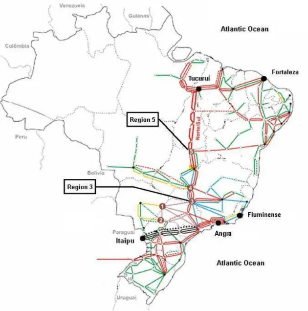
Table 5 shows the number of security constraints violated by the optimal solutions of both case studies. It is interesting to observe that a smaller number of violations occurred for all load levels inCS1. This can be explained by the network topology of the BPS, as shown in Figure 1. Most of the load is located along the east coast (Atlantic ocean), and the most important hydro plants are located in rural areas, such as the Itaipu and Tucuruí hydro plants. When economic dispatch assigns more generation to these distant hydro plants, (CS2), the long transmission lines that bring this generation to the load centers operate closer to their capacities and more se-curity constraints become active. When dispatch is designed to minimize transmission loss, (CS1), more generation is as-signed to conventional and nuclear thermal plants which are closer to the load centers, such as the Angra, Fluminense and Fortaleza thermal plants, thus reducing the power flow along the long transmission lines, resulting in less active security constraints. These shifts in generation are presented in Ta-ble 6 related to the generating units presented in Figure 1. These two case studies illustrate the trade-off in the BPS be-tween optimal dispatch from an “economic” point of view
(which maximizes hydro generation and minimizes thermal fuel costs) and optimal dispatch from an “electric” point of view (which minimizes transmission loss).
Table 5: Number of constraints violated by type on the OAPF solution
Number of violations
Load Level CS1 CS2
B G M Total B G M Total
Light 0 0 0 0 2 0 1 3
Medium 0 0 0 0 5 0 1 6
Heavy 0 0 5 5 16 2 4 22
Table 6: Generation of most important plants forCS1andCS2 Capacity [MW] Generation [MW]
Plant CS1 CS2
Itaipu 12600 3522 12412
Tucuruí 5625 1859 5510
Angra 2229 2229 1243
Fluminense 1011 1011 104
Fortaleza 391 391 0
Table 7 shows the values for the seven largest of the 22 secu-rity constraints violated in case studyCS2(heavy load).
Table 7: Most important violations forCS2(heavy load)
Violation[MW] Constraint Type Light Medium Heavy
79 B 0 0 241
84 M 0 0 760
86 G 0 0 714
111 M 0 0 408
135 B 149 534 640
155 B 46 179 274
157 M 0 0 910
Constraint 79 (Region 5 in Figure 1) is violated in Heavy level; it consists of maintaining the transformer shown in Fig. 2 in secure operation. This constraint is responsible for pre-venting the contingency that one of the three lines will cause a fault in the transformer that connects the500kV area and
230kV area. This situation corresponds to the branch out-age case mentioned in Section 3; it can be stated mathemati-cally by the following expression−3100≤ 1.00(f235−92+
f235−93+ f235−94) + 1.00f3965−230+ 1.00f235−230 ≤
3100. (matricial formsmin ≤ N f ≤ smax). Constraints
135and155represent similar situations.
Figure 1: Overview of the BPS grid.
multiple equipment congestion case mentioned in Section 3; it can be stated mathematically as−8050 ≤ f535−536 +
p500+ p501+p502+p503+ p507+p510+p513+p520≤
8050. (matricial formsmin ≤N f+M p≤smax). Similar situations are represented by constraints111and157.
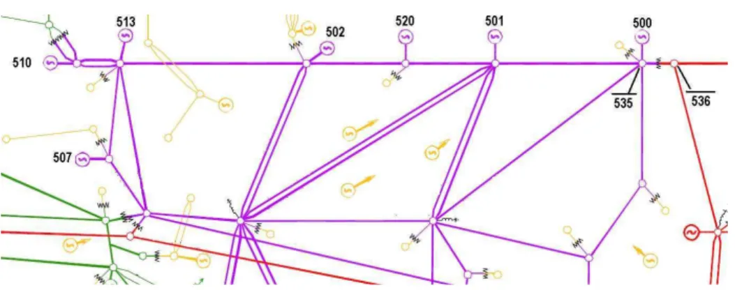
Constraint 86 (Region 3 in Figure 1) consists of the pre-vention of congestion by limiting the maximum power out-put of the group of generators shown in Fig. 3. This con-straint can be treated as a special case of multiple equipment congestion; it can be stated mathematically as −5550 ≤
p501+p502+p503+p510+p513+p520≤5550. (matricial formsmin≤M p≤smax).
6.2
SCOAPF model
A second set of numerical results is now presented to evalu-ate the proposed model when security constraints are consid-ered. Table 8 summarizes the performance of the proposed approach, which corresponds in this case to the SCOAPF model, for a heavy load. The inclusion of security constraints influenced the performance of the model in relation to the sit-uation in which these constraints were not considered (Table 3).
itera-Figure 2: Illustration of Constraint79of Region 5.
Figure 3: Illustration of constraints84and86from Region 3.
Table 8: Performance of the SCOAPF model
Time[s](Iter. OPF1/ Iter. OPF2)
Load Level CS1 CS2
Heavy 280(9/9) 998(41/24)
tion is computationally less costly. Moreover, Matrix Dy presents0.2320%of non-zero elements without security con-straints, whereas the same matrix with security constraints has0.3122%of non-zero elements (an increase of 34.57%
in the number of non-zero elements). Furthermore, the in-clusion of constraints results in an increase in the number of iterations.
Since only a few of the security constraints are active in the optimal solution, one alternative to reduce CPU time would be to adopt a scheme similar to that found in (Stott e Hob-son, 1978), in which only the security constraints actually violated, identified after running the OAPF, are included in the SCOAPF model. Note that these constraints are here si-multaneously included in the SCOAPF, although in (Stott e Hobson, 1978) they were included one at a time. The
appli-cation of this procedure forCS2and heavy load, where only 22 of the 157 security constraints are violated, reduced the CPU time of about 30%.
7
CONCLUSION
ACKNOWLEDGMENT
This research was supported in part by FAPESP, CNPq, CAPES, and FINEP, Brazilian agencies for research support.
REFERENCES
Alsac, O., Stott, B. e Tinney, W. F. (1983). Sparsity-oriented compensation methods for modified network solutions,
IEEE Transactions on Power Apparatus and Systems
PAS-102(5): 1050–1060.
Biskas, P. e Bakirtzis, A. (2004). Decentralized security con-strained dc-opf of interconnected power systems, IEE Proc.-Gener. Transm. Distrib.151(6): 747–754.
Dommel, H. W. e Tinney, W. F. (1968). Optimal power flow solutions,IEEE Trans. on PAS87(10): 1866–1876.
Expósito, A. G., Ramos, E. R. e Godino, M. D. (2006). Two algorithms for obtaining sparse loop matrices, IEEE Trans. on Power Syst.21(1): 125–131.
Granville, S. (1994). Optimal reactive dispatch through in-terior point methods,IEEE Transactions on Power Sys-tems9(1): 136–146.
Happ, H. H. (1977). Optimal power dispatch - a comprehen-sive survey,IEEE Trans. on PAS96(3): 841–854.
Harsan, H., Hadjsaid, N. e Pruvot, P. (1997). Cyclic security analysis for security constrained optimal power flow,
IEEE Trans. on Power Syst.12(2): 948–953.
Huneault, H. e Galiana, F. D. (1991). A survey of the opti-mal power flow literature,IEEE Trans. on Power Syst.
6(2): 762–770.
Jabr, R. A. (2002). A homogeneous cutting-plane method to solve the security-constrained economic dis-patching problem, IEE Proc-Gener. Transm. Distrib.
149(2): 140–144.
Lu, C. N. e Unum, M. R. (1993). Network constrained se-curity control using an interior point algorithm,IEEE Trans. on Power Syst.8(3): 1068–1076.
Mehrotra, S. (1992). On the implementation of primal-dual interior point method, SIAM Journal on Optimization
2(4): 575–601.
Momoh, J. A. (2001).Electric power system applications of optimization, Marcel Dekker, New York, NY.
Ng, W. Y. (1981). Generalized generation distribution factors for power system security evaluations, IEEE Transactions on Power Apparatus and Systems PAS-100(3): 1001–1005.
Oliveira, A. R. L., Soares, S. e Nepomuceno, L. (2003). Opti-mal active power dispatch combining network flow and interior point approaches,IEEE Trans. on Power Syst.
18(4): 1235–1240.
Quintana, V. H., Torres, G. L. e Medina-Palomo, J. (2000). Interior-point methods and their applications to power systems: Classification of publications and software codes,IEEE Trans. on Power Syst.15(1): 170–176.
Sauer, P. W. (1981). On the formulation of power distribution factors for linear load flow methods,IEEE Transactions on Power Apparatus and Systems PAS-100(2): 764– 769.
Stott, B. (1974). Review of load-flow calculation methods,
Proc. IEEE62(7): 916–929.
Stott, B., Alsac, O. e Monticelli, A. J. (1987). Security anal-ysis and optimization,Proc. IEEE75(12): 1623–1644.
Stott, B. e Hobson, E. (1978). Power system security control calculations using linear programming, part 1, IEEE Transactions on Power Apparatus and Systems PAS-97(5): 1713–1731.
Stott, B. e Marinho, J. L. (1979). Linear programming for power-system network security applications,IEEE Transactions on Power Apparatus and Systems PAS-98(3): 837–848.
Torres, G. L. e Quintana, V. H. (1998). An interior-point method for nonlinear optimal power flow using voltage rectangular coordinates, IEEE Trans. on Power Syst.
13(4): 1211–1218.
Vargas, L. S., Quintana, V. H. e Vannelli, A. (1993). A tu-torial description of an interior point method and its applications to security-constrained economic dispatch,
IEEE Transactions on Power Systems8(3): 1315–1324.
Wai, Y. (1981). Generalized generation distributions factors for power systems security evaluations, IEEE Trans. Power Syst.100(3): 1001–1005.
Wei, H. (1996). An application of interior point quadratic programming algorithm to power system optimization problems,IEEE Trans. Power Syst.11(1): 260–266.
Wood, A. J. e Wollenberg, B. F. (1996). Power generation, operation, and control, John Wiley, New York, NY.
Yan, W., Yu, J., Yu, D. C. e Bhattarai, K. (2006). A new opti-mal reactive power flow model in rectangular form and its solution by predictor corrector primal dual interior point method, IEEE Transactions on Power Delivery
21(1): 61–67.
![Table 1: BPS configuration for each load level Load Level Branches Buses Load [MW]](https://thumb-eu.123doks.com/thumbv2/123dok_br/18973709.454616/6.892.107.432.256.591/table-configuration-level-load-level-branches-buses-load.webp)