Sba Controle & Automação vol.20 número2

(1)

ROBUST CONTROL METHODOLOGY FOR THE DESIGN OF

SUPPLEMENTARY DAMPING CONTROLLERS FOR FACTS DEVICES

Roman Kuiava

∗

kuiava@sel.eesc.usp.br

Rodrigo A. Ramos

∗

ramos@sel.eesc.usp.br

Newton G. Bretas

∗

ngbretas@sel.eesc.usp.br

∗

Department of Electrical Engineering Engineering School of São Carlos University of São Paulo (USP), São Carlos, Brazil

ABSTRACT

In this paper, a new procedure to design Supplementary Damping Controllers (SDCs) for Flexible Alternating Cur-rent Transmission System (FACTS) devices is proposed. The control design problem is formulated as a search for a feasi-ble controller subject to restrictions in the form of Linear Ma-trix Inequalities (LMIs). The main objective, from the appli-cation viewpoint, is the improvement of the damping ratios associated to inter-area oscillation modes. Unlike other types of formulations existing in the literature, this new formula-tion is capable of explicitly modeling the constraints on the controller bandwidth, which are crucial to avoid undesired amplification of high frequency noise signals coming into the controller input. To illustrate the efficiency of the proposed procedure, the design of an SDC for a Thyristor Controlled Series Capacitor (TCSC) placed in the New England/New York benchmark test system is carried out. The results show the designed controllers are able to provide adequate damp-ing for the oscillations modes of interest for several different operating conditions.

KEYWORDS: Inter-area oscillations, linear matrix inequal-ities, supplementary damping controller, FACTS devices, TCSC.

Artigo submetido em 01/04/2008 (Id.: 00865) Revisado em 10/11/2008, 30/12/2008

Aceito sob recomendação do Editor Associado Prof. Julio Cesar Stacchini Souza

RESUMO

Este artigo propõe um novo procedimento para projeto de controladores suplementares de amortecimento (ou SDCs, do inglêsSupplementary Damping Controllers) para dispo-sitivos FACTS. O problema de projeto do controlador é for-mulado como uma busca por um controlador que satisfaça um conjunto de restrições na forma de desigualdades matri-ciais lineares (ou LMIs, do inglêsLinear Matrix Inequali-ties). Sob o ponto de vista de aplicação, o objetivo principal de controle é aumentar as taxas de amortecimento das osci-lações inter-área. Ao contrário de outras formuosci-lações pro-postas na literatura, esta nova formulação é capaz de mode-lar, explicitamente, as restrições da banda passante do con-trolador, evitando assim que ruídos em alta frequencia se-jam amplificados a partir do sinal de entrada do controlador. Para ilustrar a eficiência do procedimento proposto foi rea-lizado um projeto de controlador suplementar para dispositi-vos TCSC instalados no sistema New England/New York. Os resultados mostram que os controladores projetados são ca-pazes de fornecer amortecimento adequado para os modos de oscilação de interesse em diversas condições de operação.

(2)

1 INTRODUCTION

Inter-area oscillations are a common phenomenon observed in electric power systems world-wide, where groups of syn-chronous generators are interconnected over long distance transmission lines. Usually, these interconnection lines cre-ate a weak electric coupling between the generator groups and must sustain high levels of active power flow during nor-mal operation. As a consequence, the inter-area oscillations will probably exhibit poor damping (or even instability) in the absence of an adequate stabilizing control system (Kun-dur et al., 2004)(Gama, 1999). Power System Stabilizers (PSSs) have been used for many years to supply additional damping for the low-frequency oscillations in power systems by means of a stabilizing signal added to the excitation sys-tems of the generators (DeMello and Concordia, 1969). In practice, the PSSs are effective to damp local oscillations but, unfortunately, they are not always as effective to damp inter-area oscillations. This mainly occurs due to the diffi-culties related to tuning and coordination of multiples PSSs which operate in different power systems areas (Handschin, Schnurr and Wellssow, 2003). In these cases, the use of al-ternative solutions is mandatory.

In recent years, due to development of power electronics, the Flexible Alternating Current Transmission System (FACTS) devices have been successfully used to improve steady-state and dynamic system performance, and became an interesting cost-effective alternative compared to the system expansion (Paserba, 2004). These devices can be used, for example, to improve local voltage stability margins and/or to reduce elec-trical distances in long transmission lines. As a consequence, the maximum amount of active power that can be transferred among the interconnected systems may be increased. Also, there are several types of FACTS devices that may be used to provide additional damping to inter-area oscillations by inclusion of a Supplementary Damping Controller (SDC) to the device (Paserba, 2003)( Hingorani and Gyugyi, 2000).

From the practical viewpoint, there are several characteristics that both type of damping controllers (PSSs and SDCs for FACTS devices) have to possess. The following list depicts some of them:

(i) the controllers must be robust with respect to the uncer-tainties in the system operating point, i.e., a satisfactory level of damping must be achieved in several different operating conditions;

(ii) multiple damping controllers operating simultaneously in a system must have a coordinated action;

(iii) the action of the damping controllers must vanish in steady-state, so the controllers do not change the oper-ating point defined by the load flow;

(iv) a control structure based on dynamic output feedback must be used due to difficulties in obtaining measure-ments of all state variables of the system, and;

(v) it is preferable to use local input control signals, be-cause the use of remote signals would require the im-plementation of dedicated communication links and complex control schemes, which would increase the cost for implementation of the controller.

The usual practice in power systems is to employ classi-cal phase compensation to design both PSSs and SDCs for FACTS devices. These controllers consist basically of a static gain, a washout filter and a phase compensation net-work (Gama, 1999)(DeMello and Concordia, 1969). Such quite simple control structure suitably satisfies the practical requirements (iii) to (v).Ad hocapproaches are often used to tune the parameters of these controllers (as, for example, pole placement techniques based on root locus rules and eigen-value placement using transfer function residues) (DeMello and Concordia, 1969)(Larsen and Swann, 1981). The ma-jor difficulties in these design procedures are related to the practical requirements (i) and (ii), i.e., in guaranteeing the robustness of the controller with respect to the uncertainties in the system operation that were not treated in the design stage, and also to ensure an adequate coordination of multi-ple damping controllers operating simultaneously in the sys-tem.

A number of alternative techniques (based on classical and modern control concepts) have been proposed to address the robustness and coordination of multiple damping controllers. Design procedures based on frequency domain methods are presented, for example, in (IEEE Power System Engineering Committee, 1999). Methodologies based on robust control theory were also proposed, and the H∞ mixed-sensitivity formulation (Chaudhuri and Pal, 2004), the combined H∞

control problem with regional pole placement constraints us-ing LMIs (Tsai, Chu and Chou, 2004) and the multi-objective genetic algorithms approach (Bomfim, Taranto and Falcão, 2000), can be cited as examples.

Paper (Ramos, Alberto and Bretas, 2004a) proposes a methodology (which was later on extended in (Ramos, Mar-tins and Bretas, 2003)), based on a robust control technique, to design PSS-type controllers. The design objective of such methodology consists basically in calculating a dynamic out-put feedback controller described in state space form by ma-trices AC, BCand CCthat stabilize (also fulfilling a specific

(3)

guaran-tee both: robustness (using the Polytopic Quadratic Stabil-ity concept) and a minimum performance of the closed loop system by means of a Regional Pole Placement technique (Boyd et al., 1994)(Chiali, Gahinet and Apkarian, 1999). As a result, the control formulation is described by a set of BMIs (Bilinear Matrix Inequalities) on the matrix variables. It is possible, however, to transform these BMIs into a set of LMIs by a two-step separation procedure shown in (Oliveira, Geromel and Bernussou, 2000).

The resulting control methodology based on LMIs is pre-sented in (Ramos, Alberto and Bretas, 2004a) for the design of PSS-type controllers. Unfortunately, this control method-ology is not general enough to be applied in the design of SDCs for FACTS devices. In reference (Xue, Zhang and Godfrey, 2006) a different two-step separation procedure is applied, and the resulting procedure is able to handle the problem of SDC design for FACTS devices. It is also argued in (Xue, Zhang and Godfrey, 2006) that the ideas used in (Ramos, Alberto and Bretas, 2004a) and (Oliveira, Geromel and Bernussou, 2000) may not be applicable to this problem.

This paper proves the converse, i.e., that the ideas in (Ramos, Alberto and Bretas, 2004a) and (Oliveira, Geromel and Bernussou, 2000) can indeed be applied to derive a procedure capable of handling the design of supplementary controllers in general (that is, either PSS-type controllers or SDCs for FACTS devices). Furthermore, it also includes an explicit formulation to ensure that the bandwidth of the resulting con-trollers is acceptable in practice, which is very important to avoid the amplification of high frequency noise signals in the controller input. These two features constitute the main con-tribution of this paper.

The paper is structured as follows: section 2 reviews the fun-damentals of the control methodology proposed in (Ramos, Alberto and Bretas, 2004a), and shows why it is not appli-cable to the design of SDCs for FACTS devices; section 3 presents the proposed control technique, which is based on the ideas developed in (Ramos, Alberto and Bretas, 2004a); section 4 summarizes the complete design procedure; results of the tests performed using the proposed procedure are pre-sented in section 5, and section 6 presents the conclusions and the final comments.

2 THE PREVIOUSLY PROPOSED

CON-TROL METHODOLOGY

This chapter presents a review of the main fundamentals about the previously proposed control methodology, which was developed in (Ramos, Alberto and Bretas, 2004a) for designing PSS-type controllers.

2.1 System and Controller Models

The power system model is represented in (Ramos, Alberto and Bretas, 2004a) by a set of nonlinear differential and al-gebraic equations in the form

˙

x=f(x, z, u), (1)

0=g(x, z, u), (2)

y=h(x, z, u), (3)

wherex(t) ∈ ℜn is a vector composed of the system state variables, z(t) ∈ ℜm is a vector of algebraic variables,

u(t) ∈ ℜp

is a vector with the system control input, and

y(t)∈ ℜq

is the vector with the system outputs.

Usually, the analyses of local and inter-area oscillations and design of damping controllers for power systems are carried out by means of linear models (Chaudhuri and Pal, 2004). The process often involves linearizing the system equations (1)-(3) around a specific equilibrium point. The vector of algebraic variableszis eliminated by isolating it and substi-tuting the result in the linearized equation obtained from (1). Using this process, a linear representation of the system in the vicinity of the equilibrium point is obtained, which can be described in state space form by

˙

x(t) =Ax(t) +Bu(t), (4)

y(t) =Cx(t). (5)

A control structure based on dynamic output feedback is adopted in (Ramos, Alberto and Bretas, 2004a). Such control structure is necessary due to difficulties in obtaining mea-surements of all model state variables in the real system. The proposed controller based on dynamic output feedback is represented by

˙

xC(t) =ACxC(t) +BCy(t), (6)

u(t) =CCxC(t), (7)

wherexC(t)∈ ℜn

is a vector with the controller states. The dynamic behavior of the controller, as a function of the plant outputy(t), is described by (6). The control input for the systemu(t) is produced by (7) with the application of the matrix gainCCto the states generated by the controller.

2.2 Control Problem Formulation

(4)

˙˜

x(t) =A˜˜x(t), (8)

where

˜ A=

A BCC

BCC AC

, (9)

andx(t˜ )∈ ℜ2nis a vector with the states of both the system and the controllers. Notice thatAC, BC, and CC are the matrix variables to be determined by the design procedure.

Using the Lyapunov stability theory for linear systems, the problem of stabilizing the system (4)-(5) by the output feed-back controller (6)-(7) can be solved (Skelton, Iwasaki and Grigoriadis, 1998) if the controller matricesAC,BC, CC and a matrixP˜ = P˜T > 0 (with appropriate dimensions) are found, such that

˜

ATP˜+P ˜˜A<0. (10)

This idea constitutes the core of most design procedure based on Lyapunov stability theory for linear systems. However, this simple formulation is not adequate to the design of damping controllers for power systems, because:

(i) The controller designed using (10) may not provide a satisfactory damping to the oscillation modes of inter-est since no performance index is considered in that for-mulation;

(ii) since the linear approximation (4)-(5) is valid only in a vicinity of a particular operating point, the robustness of the controller with respect to the variations in the operating conditions of the system is very limited;

(iii) inequality (10) is a Bilinear Matrix Inequality (BMI) on the problem matrix variables (AC,BC, andCCand

˜

P), whose solution may require a large computational effort.

Each of these problems was addressed in (Ramos, Alberto and Bretas, 2004a) using suitable extensions of the core idea expressed in (10). The next subsections present a brief overview of these extensions.

2.3 Performance Index

In (Ramos, Alberto and Bretas, 2004a), a performance crite-rion (in the form of a minimum damping ratio to be achieved for all modes of the closed loop system) is included in the

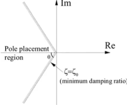
control formulation to ensure an acceptable performance for the controlled system. This inclusion is done using the Re-gional Pole Placement (RPP) technique (Chiali, Gahinet and Apkarian, 1999), which consists in the definition of a region for pole placement in the complex plane where the perfor-mance criterion is fulfilled. This region is defined byζ≥ζ0, and it can be viewed in Fig. 1, whereζ0is the desired mini-mum damping ratio for the poles of the closed loop system.

Figure 1: Region for the pole placement.

The pole placement criterion expressed in Fig. 1 can be ful-filled if matricesAC,BC,CCandP˜ =P˜T >0are found such that the BMI (Ramos, Alberto and Bretas, 2004a)

"

sinθ·A˜TP˜+P ˜˜A cosθ·(P ˜˜A−A˜TP)˜ cosθ·(A˜T_˜

P−P ˜˜A) sinθ·(A˜T_˜

P+P ˜˜A)

#

<0,

(11)

is satisfied, whereθ= cos−1_(ζ0)_{and matrices}_A˜_and_P˜_were

previously defined.

2.4 Performance Robustness

The uncertainties in the power system model with respect to the variations of the operating conditions were treated in (Ramos, Alberto and Bretas, 2004a) using the polytopic modelling technique (Boyd et al., 1994)(Ramos, Bretas and Alberto, 2002). In this technique, instead of using a single Linear Time Invariant model, the system is modeled by a Polytopic Linear Differential Inclusion in the form

˙˜

x∈A(a)˜˜ x, (12)

whereA(a)˜ ∈ΩandΩis a closed subset of a matrix space with dimension2n×2n,which is formed by the convex com-bination of a set of predefined matricesA˜i. Notice that each

˜

Ai comes from a closed loop representation of the power

(5)

around a particular operating condition. Such operation point may be chosen, for example, from the load curve of the sys-tem, complying with the typical practice in the industry. Set

Ωcan be written as

Ω=

(

˜

A(a) :A(a) =˜ L

X

i=1 aiAi;˜

L

X

i=1

ai= 1;ai≥0

)

.

(13)

It can be observed in (13) that setΩis a polytope in the ma-trix space and matricesAi˜ are the vertexes of this polytope, beingLthe number of operating points used for the construc-tion of the polytope.

Using both polytopic modelling and RPP technique in the design procedure, associated with the quadratic stability the-ory (Boyd et al., 1994), an adequate damping of the oscil-lation modes of the system is guaranteed. This is achievied not only for the operating points used as vertexes in the con-struction of the polytopic model, but also for all the operat-ing points that can be generated from the convex combina-tion of these operating points (Ramos, Bretas and Alberto, 2002)(Barmish, 1985). Such statement is satisfied solving the following BMIs on the matrices variablesAC,BC,CC andP˜(which must be symmetric):

˜

P>0, (14)

"

sinθ·A˜T_i P˜+P ˜˜Ai cosθ·(P ˜˜Ai−A˜T_i P)˜ cosθ·(_A˜T

i P˜−P ˜˜Ai) sinθ·(A˜

T

i P˜+P ˜˜Ai)

#

<0,

(15)

where Ai=˜

Ai BiCC

BCCi AC

,i = 1, ..., L and θ = cos−1_(ζ0)_.

The matrix inequalities (14)-(15) are BMIs on the problem matrix variablesAC,BC,CC andP˜. However, such ma-trices inequalities can be transformed to a set of LMIs us-ing a two-step separation procedure (Oliveira, Geromel and Bernussou, 2000). This procedure consists basically in a pa-rameterization and a change of some matrix variables of the control formulation (14)-(15), allowing the solution of the inequalities by two sequential steps. The first one involves a choice of matrixCCand the second one consists in finding matricesACandBCusing the previous choice ofCC. However, as originally proposed in (Ramos, Alberto and Bre-tas, 2004a), this design procedure was conceived to work over polytopic models whose vertices were comprised by lin-ear models in the form (4)-(5), leading to the closed loop for-mulations in the form (8). These closed loop forfor-mulations are

not suitable for the problem of SDC design for FACTS de-vices, because the linearized models of power systems con-taining these devices usually exhibit a direct feedthrough ma-trix D in the output equation. For this reason, it was argued in (Xue, Zhang and Godfrey, 2006) that the ideas support-ing the procedure proposed in (Ramos, Alberto and Bretas, 2004a) may not be applied to design SDCs for FACTS de-vices. The next section proves this statement wrong, and proposes a new formulation (which uses the main ideas from (Ramos, Alberto and Bretas, 2004a)) which is not only ca-pable of designing such controllers, but is also caca-pable of handling constraints on the controller bandwidths, which are very important from the practical point of view.

3 THE PROPOSED NEW CONTROL

FOR-MULATION

In order to be able to handle the design of SDCs for FACTS devices, the new control formulation proposed in this paper deals with generalized power system models with matrices

A,B,Cand also a non-zero matrixD.

For that, consider again the linearized power system model described by (4)-(5). The time derivative of active power measurements is used as input control signal. This signal ex-hibits a great observability of the inter-area oscillations of interest and, additionally, its derivative effect prevents the controller from acting in steady-state (Ramos, Alberto and Bretas, 2004a)(Ramos, Alberto and Bretas, 2004b). There-fore, the practical requirement (iii) in the list presented in section I is fulfilled. The time derivative of the outputy(t)

can be written as

¯

y(t) = ˙y(t) =_{Cx(t) +}¯ _Du(t),¯ ₍₁₆₎

whereC¯ =CAandD¯ =CBare matrices with dimensions determined byA,BandC. Besides,D¯ is a non-zero matrix for the FACTS devices due to the sensibility of the line active power flow to variations in the FACTS controllable parame-ters (as for example, the equivalent reactance for a TCSC device). It is important to point out that the definition of the new output as the time derivative of the previous one does not require the implementation of an ideal derivative block. As explained in (Ramos, Alberto and Bretas, 2004b), this derivative action can be later incorporated into the controller transfer function to compose a washout block, which is typi-cal of PSSs and SDCs for FACTS devices.

With this new definition for the output, the dynamics of the controller can now be described by

˙

(6)

Figure 2: Region for the pole placement.

From the connection of the power system model (4) and (16) with the damping controller model (17)-(7), the vertices of the polytope for the controlled system with general power system models described by the set (A,B,C,¯ D)¯ will be given by

˜ Ai=

Ai BiCC

BCCi¯ AC+BCDiC¯ C

, (18)

fori= 1, ..., L.

Furthermore, as mentioned earlier, an additional practical re-quirement is included in the control formulation to ensure that the controller bandwidth remains within acceptable lim-its. With this inclusion, the new region of the complex plane used for the pole placement is shown in the Fig. 2 as re-gion D, which is delimited by a circle with radiusr and a conic sector defined by angleθ. So, such region ensures a minimum damping ratioζ0= cosθ(ensuring the oscillation modes are adequately damped) and a maximum natural os-cillation frequencyw=rsinθ(ensuring that the closed loop system has acceptable bandwidth) for the poles of the poly-topic closed loop model.

The matrices inequalities related to the polytopic modelling (considering the generalized power system model) and the RPP technique with the constraints shown in Fig. 2, are given by (Chiali, Gahinet and Apkarian, 1999)

˜

P>0, (19)

−rP˜ P ˜˜Ai ˜

AT

i P˜ −rP˜

<0, (20)

"

sinθ·A˜T

i P˜+P ˜˜Ai

cosθ·(_{P ˜}˜_Ai₋_A˜T

i P)˜ cosθ·(A˜T

i P˜−P ˜˜Ai) sinθ·(A˜

T

i P˜+P ˜˜Ai)

#

<0,

(21)

where

˜ Ai=

Ai BiCC

BCCi¯ AC+BCDiC¯ C

, i= 1, ..., L, θ=

cos−1_(ζ0)_and_r_{is a scalar}_.

So, if matricesAC,BC,CCof the proposed controller and also a matrixP˜ = P˜T

> 0 (defining an appropriate Lya-punov function) are found, such that (19) to (21) are satis-fied, the poles of the controlled system are confined into the region D of the complex plane, not only for the operating points used in the construction of the polytopic system, but also, for all the operating points that can be generated from the convex combination of the L adopted operating points.

The next section shows how to use the two-step procedure in (Oliveira, Geromel and Bernussou, 2000) to transform the set of BMIs (19)-(21) into a set of LMIs which corresponds to the generalized control formulation proposed in this paper.

3.1 The Two-step Separation Procedure

The concepts and procedures described in this section are derived from the ideas presented in (Oliveira, Geromel and Bernussou, 2000). The first stage of the separation proce-dure consists in setting up a state feedback gain that stabi-lizes the polytopic system with the pole placement objec-tives discussed previously. For that, it is possible to find a state feedback gainKf=LY

−1

solving the following LMIs in the matrices variablesLandY(Ramos, Alberto and Bre-tas, 2004a):

Y >0, (22)

₋

rY AiY+BiL

∗ −rY

<0, (23)

     

sinθ·(YAT_i +AiY +LT

BT

i +BiL)

cosθ·(YAT_i −AiY +LT

BT

i −BiL)

cosθ·(−YATi +AiY −LTBTi +BiL)

sinθ·(YATi +AiY +LT

BTi +BiL)

     

<0, (24)

where i = 1,...,L andris a scalar. Then, the first step of the separation procedure is concluded definingC¯C := Kf as being the output matrix of the proposed damping controller.

For the second step of the separation procedure, considers the BMIs (19) to (21). It is possible to partitioned the symmetric matrixP˜ and its inverse P˜−1_{according to the dimensions}

(7)

˜ P=

X U

UT

XC

, P˜−1

=

Y Y

Y YC

, (25)

whereX,XC,Y,YC,U∈ ℜnxn. Now, letT∈ ℜ2n

×2n _a

matrix defined by

T=

I I I 0

, (26)

where the dimensions of the submatrices are implicitly deter-mined byP˜.

Moreover, the following changes of variables are carried out

F=UBC,P=Y

−1

,S=ATCU T

, (27)

where the dimensions of the matricesF,PandSare implic-itly determined by the transformations.

Now, the BMIs (19)-(21) can be transformed into a set of LMIs. For that, multiply these BMIs on the right and the left byT˜ =diag[T,T], introduce the new variablesF,P,

Sand simplifies the expression by algebraic manipulations, remembering thatP ˜˜P−1 = I. Solving the set of LMIs ob-tained by such development in the matrices variablesF,P,

SandX, the matricesACandBCof the proposed damp-ing controller can be calculated by (27), whereU=P−X. The set of LMIs are given by

P P P X

<0, (28)

   

−rP −rP PAki¯ PAi

∗ −rX XAki¯ +FCki¯ +S XAki+FT

CT

∗ ∗ −rY −rI

∗ ∗ ∗ −rX

   

<0,

(29)

   

N11 N12 N13 N14

∗ N22 N23 N24

∗ ∗ N33 N34

∗ ∗ ∗ N44

   

<0, (30)

where

N11=sinθ· (PA¯+_kiA¯T kiP), N12=sinθ· (PA¯+i A¯

T

kiX+ ¯C_kiFT T ₊_S),

N13=cosθ ·( ¯ATkiP −PA¯)ki, N14=cosθ·(−P A+i A¯

T

kiX+ ¯C_kiFT T₊_S), N22=sinθ·(XA+i A

T

iX+FC¯ + i C¯

T i F

T_),

N24=cosθ·(−XA+i A T

iX−FC¯i+C¯ T i F

T ), N23=NT

14, N33=N ,

11N34=N ,

12N44=N , 22 ¯

Aki=Ai+BiCC¯ ,

¯

Cki = ¯Ci + ¯DiCC,¯ (i = 1, ..., L), withCC¯

calculateda prioriby (22)-(24).

The next section presents the complete design procedure based on the developments described previously.

4 THE DESIGN PROCEDURE

The design procedure is divided in three stages: (i) construc-tion of the polytopic model; (ii) calculaconstruc-tion of the state feed-back gain matrix of the controller (CC) and; (iii) calculation of the matrices that describe the controller dynamics (matri-cesACandBC). Each stage is described in this section.

4.1 Construction of the Polytopic

Mod-elling

The first step of the controller design procedure consists in choosing some typical operating points of the system to ob-tain the matricesAi˜ (i= 1, ..., L)that define the vertexes of the polytopic model. The steps for carrying out the first stage are:

(i) Build the power system model as a set of nonlinear dif-ferential and algebraic equations in the form (1)-(3);

(ii) Linearize the system equation (1)-(3) around L equilib-rium points and after the network reduction (which is required to eliminate the vector of algebraic variables

z), theLlinear systems are obtained in the space state form which will constitute the vertexes, as in (12), of the polytopeΩ.

4.2 Calculation of the State Feedback

Gain Matrix of the Controller (Matrix

CC

)

(8)

AC,BCandCC. This controller must stabilize the polytope

Ωwhile fulfilling a minimum damping ratio and a maximum natural oscillation frequency for all modes of the closed loop polytopic model. In this design stage, the state feedback gain matrix of the controllers (CC) is determined by means of the solution of a set of LMIs written for the polytope vertexes. These steps can be carried out in the following way:

(i) Define the minimum damping ratioζ0 = cosθ and a maximum frequencywm=rsinθ. Therefore, a region in the complex plane defining the minimum acceptable performance index is specified for all the oscillation modes of the polytopic system (according to Fig. 2); (ii) build the computational representation of the matrix

variablesL andY. The matrixYmust be symmetric with dimensionn×nand the matrixLmust be rectan-gular with dimensionp×n. The set of LMIs (22)-(24) must be structured and solved for the variablesLand Y;

(iii) after determining the variables L and Y, the state feedback gain matrix CC can be calculated by

¯

CC=LY− 1

.

In the next stage, the matricesAC andBC are calculated with the previously designed matrixCC.

4.3 Calculation of the Matrices A

C

and B

C

In the last stage, the matrices AC and BC are calculated by means of the solution of a new LMI set established in the polytope vertexes. To do so, the following steps must be executed:

(i) Build the computational representation of the new ma-trices variablesF,P,SandX,with dimensionsn×n,

n×n,n×qandn×n, respectively, and solve the set of LMIs (28)-(30) in these variables;

(ii) After findingF,P,SandX, the matricesACandBC can be calculated byAC=U−1

ST

andBC=U−1

F, whereU=P−X.

After concluding the three design stages, the matricesAC,

BC andCCwhich define the structure of the SDC for the FACTS device are obtained. Such controller can also be rep-resented in the transfer function form obtained by

H(s) =CC(sI−AC)

−1

BC. (31) With the purpose of implement the transfer function (31) without using the time derivative of the output∆yobtaining

the desired time derivative of the line active power (without the inclusion of an ideal derivative block) as input control signal, it is possible to rewrite (31) in the zeros/poles/gain form, as the following relation shows (Ramos, Martins and Bretas, 2005):

¯ H(s) =K

Qz

k=1(zk+s)

Qp

l=1(pl+s)

=K Tw

1 +sTw

Qz

k=1(zk+s)

Qp−1

l=1 (pl+s) ,

(32)

whereKis the gain, whilepandzare, respectively, the num-ber of poles and zeros of the controller. The parameterTwis equal to−1/ph, whereph must be chosen as the real pole placed closest to the origin by the controller design proce-dure. Since that∆u =_H(s)∆¯¯ _y ₌_s_H(s)∆y¯ _{, we can}

im-plement the designed controller from the active power mea-surements by:

∆u=K sTw 1 +sTw

Qz

k=1(zk+s)

Qp−1

l=1 (pl+s)

∆y. (33)

5 TESTED SYSTEM

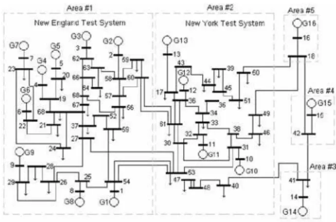
To demonstrate the effectiveness of our proposed proce-dure, tests were carried out on a 16-machine, 5-areas sys-tem, shown in Fig. 3. This is a reduced order model of the New England and New York interconnected system. The first nine machines (G1 to G9) are the generators associated with the New England Test System (NETS), while G10 to G13 are the generators of the New York Power System (NYPS). Also, G14 to G16 are representing three equivalent areas neighbor-ing connected to the NYPS.

In the adopted multimachine model, all the generators were described by a sixth order model that considers the swing equations and the transient and subtransient effects indand

qaxes (Anderson and Fouad, 1994).

Also, the machines were equipped by a first order model of a static type AVR (thyristor controlled without transient gain reduction) with a gain equal to 50 and a constant time of 0.01s. The transmission system was modeled as a pas-sive circuit by means of algebraic equations and the system loads were modeled as constant impedances. The data for bus, lines and machines were taken from (Pal and Chaudhuri, 2005).

(9)

func-Figure 3: 16-machine, 5 areas study system.

tion residues (IEEE Power System Engineering Committee, 1999).

Since our main purpose is to design SDCs for FACTS de-vices, we chose one type of such devices that is regarded as a highly effective solution to improve damping of inter-area oscillations (a task that PSS sometimes cannot per-form with similar effectiveness): the well-know Thyristor Controlled Series Capacitor (TCSC). In our application, the TCSC is represented by a first order linear model (Del Rosso, Canizares and Dona, 2003) (which is a typical model used in small-signal stability studies). The block diagram of the adopted TCSC with an SDC is given in Fig. 4.

In Fig. 4,∆XT CSC is the deviation of the equivalent TCSC reactance with respect to the nominal value,∆Xref is the reference for the desired reactance deviation (from its nom-inal value) in steady state, ∆Xsup is the stabilizing signal from the proposed supplementary controller andTT CSC is the device time constant.

Two TCSC devices were placed in the system with the purpose of improving the stability of inter-area oscillation modes, as well as increasing the active power transfer ca-pacity among the power systems areas. One of them was installed in the line connecting buses #60 and #61 and the other in the line connecting buses #18 and #49. Hence, the one is responsible to raise the active power transfers capacity between areas #2 and #5. The compensation of both TC-SCs (in steady-state) corresponds to 50% of the impedance of their respective lines.

All the small-signal stability analyses in this paper were car-ried out for a daily load curve, which is shown in Fig. 5. The stability of local and, especially, inter-area modes were inves-tigated in twenty-four operating points, each one equivalent to an hour of the day. The data for a particular load level (which was assumed, in this paper, as the operating

condi-Figure 4: Small-signal dynamic model of TCSC with a Sup-plementary Damping Controller (SDC).

Figure 5: Daily load curve of the tested system

tions at 3 p.m) were taken from (Pal and Chaudhuri, 2005). The other operating points were obtained using percentual variations (as shown in Fig. 5) of the system loads with re-spect to the operating conditions at 3 p.m. The generators were redispached in each of these points, sharing portions of total load variation in a direct proportion of their respective inertia constants. It was also assumed (to comply with the usual practice in power systems) that each area is responsi-ble for supplying its own load variations and, therefore, the active power flows among the areas were kept constant for all operating conditions.

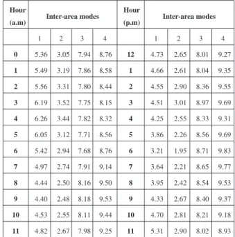
The eigenvalue analysis shows (for all considered operating conditions) that the system without the inclusion of SDCs for the TCSCs have all the local modes and also two inter-area modes adequately damped (corresponding to a damping ratio greater than 5%, which is typically accepted as an indicator of satisfactory power system dynamic behavior). These re-sults for the inter-area modes are shown in Table 1. As it can be seen, modes 3 and 4 are the well damped ones. On the other hand, mode 1 exhibits an unacceptable damping ra-tio in the operating condira-tions from 7 a.m to 10 p.m, while mode 2 is poorly damped for all the analyzed daily load curve points. The frequency of each oscillation mode is approxi-mately (since it changes with variations in the operating con-ditions) 0.74 Hz, 0.55 Hz, 0.80 Hz and 0.42 Hz, for modes 1, 2, 3 and 4, respectively.

(10)

installed between areas #1 and #2 is responsible to improve the stability of mode 1. Similarly, the TCSC installed in area #2 and also equipped with a SDC must supply an additional damping to the mode 2. Both SDCs were designed (but not simultaneously) by the proposed control methodology.

The power system model has 140 states. In order to reduce the dimensions of the power system models used to design the proposed controllers, two simplified models were devel-oped. The first one corresponds to the NETS model con-nected to a single equivalent generator (which is an equiva-lent representation of areas #2, #3, #4 and #5) and it was used to design the SDC for the TCSC installed between buses #60 and #61. This simplified model, i.e, the NETS model with the single equivalent generator, has 77 states and it is denoted in this paper by reduced modelA. Similarly, the other sim-plified power system model corresponds to the NYPS model connected to a single equivalent generator representing area #1, and it was used to design the SDC added to the TCSC installed between areas #2 and #5. This model has 66 states and it is denoted by reduced modelB.

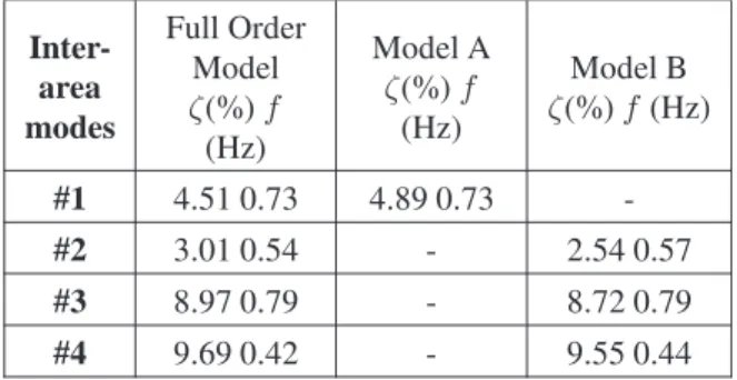
To illustrate the accuracy among the full order model (with 140 states) and the reduced models A and B, Table 2 shows the inter-area modes calculated for each of these models in the operating conditions at 3 p.m. Notice that only mode 1 is observed in the reduced model A, since the dynamics among the generators of areas #2, #3, #4 and #5 are not being con-sidered by such model. Comparing the inter-area modes cal-culated by each power system model, it is possible to verify that the reduced models A and B offer an acceptable approx-imation of the system dynamics of interest.

The proposed controllers were not designed simultaneously1, i.e., the SDC for the TCSC installed between areas #1 and #2 was designed using the reduced modelA, while the SDC for the TCSC located between areas #2 and #5 was designed us-ing the reduced modelB. For both SDCs, the time derivatives of local active power measurements were used as input con-trol signal. The operating points at 3 p.m and 4 p.m were used for the construction of the polytopic model adopted for the reduced modelA, while operating points at 5 p.m and 6 p.m were used for the polytopic model of reduced modelB. A minimum damping ratio of 5% (ζ0=0.05) and a maximum natural oscillation frequency ofr= 20 rad/s was defined as an acceptable performance index for the controlled polytopic system.

1_{Although from a theoretical viewpoint there is no restriction for the}

simultaneous design of both controllers in this case using block-diagonal structures for the controller matrices, it was tried this simultaneous ap-proach with several different block-diagonal choices but none of them produced satisfactory results. For this reason, it was chosen to apply this sequential design approach, which ended up producing better re-sults in this case.

The “feasp” solver, available in Matlab LMI Control Tool-box (Gahinet et al., 1995) was used to solve the set of LMIs related to the control problems. The time taken to generate the controllers was approximately 8 hours and 25 minutes for the SDC added to the TCSC installed between areas #1 and #2 and 4 hours and 37 minutes for the other SDC. Both set of LMIs were solved in a computer with a Pentium Dual Core 3.2 GHz processor and 2 GB of RAM.

Table 1: Damping ratios (%) of the inter-area modes for the daily load curve without the inclusion of SDCs.

Hour

(a.m) Inter-area modes

Hour

(p.m) Inter-area modes

1 2 3 4 1 2 3 4

0 5.36 3.05 7.94 8.76 12 4.73 2.65 8.01 9.27

1 5.49 3.19 7.86 8.58 1 4.66 2.61 8.04 9.35

2 5.56 3.31 7.80 8.44 2 4.55 2.90 8.36 9.55

3 6.19 3.52 7.75 8.15 3 4.51 3.01 8.97 9.69

4 6.26 3.44 7.82 8.32 4 4.25 2.55 8.33 9.31

5 6.05 3.12 7.71 8.56 5 3.86 2.26 8.56 9.69

6 5.42 2.94 7.68 8.76 6 3.21 1.95 8.71 9.83

7 4.97 2.74 7.91 9.14 7 3.64 2.21 8.65 9.77

8 4.44 2.50 8.16 9.50 8 3.95 2.42 8.54 9.53

9 4.40 2.48 8.18 9.53 9 4.33 2.67 8.40 9.37

10 4.53 2.55 8.11 9.44 10 4.70 2.81 8.21 9.18

11 4.82 2.67 7.98 9.25 11 5.31 2.90 8.02 8.93

One of the difficulties associated with the proposed design methodology is its requirement, due to the nature of the con-trol problem formulation, that the order of the designed SDC must be equal to the order of the power system model. In the presented application, since the reduced power system models A and B have, respectively, 77 and 66 states, the re-sulting SDCs had also order 77 and 66. However, high order controllers are difficult to implement in practice and, for this reason, it is desirable to reduce the dimensions of the con-trollers designed by this proposed methodology.

To achieve the goal of producing a low order controller, the proposed procedure was combined with a final step of model order reduction. After a high order controller was designed, the balanced truncation method (Pal and Chaudhuri, 1995) was applied, reducing the dimension of the SDCs from order 77 and 66 to only order 5 for both controllers.

(11)

sat-Table 2: Damping ratios (%) of the inter-area modes for the daily load curve in each of the power system models.

Inter-area modes

Full Order Model

ζ(%)f

(Hz)

Model A

ζ(%)f

(Hz)

Model B

ζ(%)f(Hz)

#1 4.51 0.73 4.89 0.73

-#2 3.01 0.54 - 2.54 0.57

#3 8.97 0.79 - 8.72 0.79

#4 9.69 0.42 - 9.55 0.44

isfy the region for pole placement (Fig. 2). In this case, it is important to verify if the bandwidth of the reduced order controller remains within acceptable limits. The validation of the effectiveness of the reduced order SDCs was carried out by comparison of the frequency responses of the full and reduced order controllers and by quadratic stability analysis with regional pole placement constraints (using the formula-tion given by (21)-(22) and considering the same polytopes adopted in design stage). The transfer functions of the re-duced order SDCs are presented in the appendix.

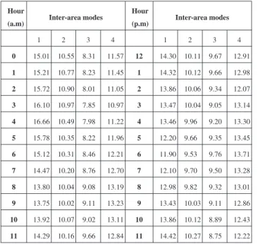
The damping ratios of the inter-area modes for the system with the inclusion of the SDCs for the TCSCs in all twenty-four operating conditions corresponding to the daily load curve analyzed previously are shown in Table 3. These re-sults were obtained considering the full order model of the power system, in which generator 13 was taken as the angu-lar reference for the system model.

Such results were also compared with conventional SDCs based on phase compensation (Pal and Chaudhuri, 2005). The structure of these SDCs consists basically of a static gain, a washout filter and a phase compensation network (formed by two lead-lag blocks). The compensation angle used to determine the lead-lag parameters was determined using the transfer function residues calculated for the base case (Pal and Chaudhuri, 2005). The damping ratios of the inter-area modes for the system with the inclusion of the con-ventional SDCs for the TCSCs are shown in Table 4.

It was verified that the performance index obtained by the TCSCs equipped with the proposed SDCs is better than the minimum acceptable performance specified in the design stage. Notice that modes 1 and 2 present now a damping ratio varying from 11.9% to 16.66% and 9.53% to 10.97%, respectively. Additionally, the TCSC installed between areas #2 and #5 and equipped with the proposed SDC well im-proved the damping ratio of mode 4 as well. On the other hand, comparing the results shown in Tables 3 and 4, it can

be seen that the performance index achieved by the conven-tional SDCs is smaller than the one obtained from the pro-posed SDCs. Indeed, for the operating conditions from 5 to 8 p.m., the damping ratios achieved by the conventional SDCs is smaller than 5%, and it is very difficult to manu-ally tune these SDCs to achieve greater damping ratios under these conditions.

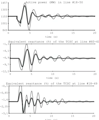
The results of the nonlinear simulation in three different op-erating conditions (at 6 p.m, 1 p.m and 3 a.m) with the pro-posed SDCs (and the conventional SDCs) are shown in Figs 6, 7 and 8. These simulations were carried out to validate the results of the linear analyses and the robustness requirement. The perturbation used to stimulate the inter-area modes was a three-phase solid fault in one of the lines connecting buses 47 and 48. The fault conditions were simulated after 2s for a duration of 80 ms (≈5 cycles in a 60 Hz system) followed by opening of the faulted line.

According to Figs. 6, 7 and 8, the TCSCs equipped with the designed SDCs presented a betted performance in com-parison with the conventional SDCs. Notice that the perfor-mance of the proposed controllers was satisfactory for oper-ating conditions that were not considered in the design stage (1 p.m and 3 a.m). This is a good indication of the robust-ness of the proposed controllers with respect to variations in the operating conditions. Additionally, the stabilizing signal provided by the SDC added to the TCSC placed between ar-eas #1 and #2 was able to reduce the maximum valor of the active power at line #60-61 in the first oscillation occurred after the perturbation.

6 CONCLUSION

A robust control methodology structured in the form of lin-ear matrix inequalities (LMIs) was presented for the design of SDCs for FACTS devices, with the purpose of improving the stability of inter-area oscillation modes. This required the development of a new formulation, based on the ideas explored by the authors in previous works, that is now capa-ble of treating the models that arise when FACTS devices are placed in the power system. This new formulation is general enough to allow the design of either SDCs for FACTS de-vices or PSS-type controllers and also includes a further step of model order reduction, addressing the problem of con-troller order, which was until now a drawback of the previous proposition.

(12)

ad-Table 3: Damping ratios (%) of the inter-area modes for the daily load curve with the designed SDCs (using the proposed design procedure).

Hour

1 2 3 4 1 2 3 4

0 15.01 10.55 8.31 11.57 12 14.30 10.11 9.67 12.91

1 15.21 10.77 8.23 11.45 1 14.32 10.12 9.66 12.98

2 15.72 10.90 8.01 11.05 2 13.86 10.06 9.34 12.07

3 16.10 10.97 7.85 10.97 3 13.47 10.04 9.05 13.14

4 16.66 10.49 7.98 11.22 4 13.46 9.96 9.20 13.30

5 15.78 10.35 8.22 11.96 5 12.20 9.66 9.35 13.45

6 15.12 10.31 8.46 12.21 6 11.90 9.53 9.76 13.71

7 14.47 10.20 8.76 12.70 7 12.10 9.70 9.50 13.28

8 13.80 10.04 9.08 13.19 8 12.98 9.82 9.32 13.01

9 13.75 10.02 9.11 13.23 9 13.43 10.03 9.11 12.86

10 13.92 10.07 9.02 13.11 10 13.86 10.12 8.89 12.43

11 14.29 10.16 9.66 12.84 11 14.42 10.27 8.75 12.22

vancement that comprises the set of contributions of this pa-per.

Given that the closed loop poles and zeros produced by the method may change when the controller order reduction is applied, the development of new procedures that enable the design of low-order controllers without requiring balanced truncation is one of the future directions of this research. An-other predicted development is the imposition of bandwidth restrictions only to the controller transfer function, instead of the whole closed loop system, which may improve the feasi-bility of the control problem formulation.

REFERENCES

Anderson, P. M. and Fouad, A. A. (1994). Power System Control and Stability, IEEE Press, Piscataway, USA.

Barmish, B.R. (1985). Necessary and Sufficient Condi-tions for Quadratic Stabilizability of an Uncertain Sys-tem,Journal of Optimization Theory and Applications

46(4): 399–408.

Boyd, S., El Gahoui, L., Feron E., et al (1994).Linear Ma-trix Inequalities in System and Control Theory, SIAM, Philadelphia, USA.

Bomfim, A. L. B., Taranto, G. N. and Falcao, D. M. (2000). Simultaneous Tuning of Power System Damping

Con-Table 4: Damping ratios (%) of the inter-area modes for the daily load curve with the designed SDCs (using a classical control methodology).

Hour

1 2 3 4 1 2 3 4

0 6.88 6.00 7.91 9.70 12 5.58 5.56 8.80 11.00

1 8.29 6.06 7.81 9.54 1 5.51 5.54 8.83 11.00

2 6.06 6.08 7.83 9.61 2 5.49 5.53 8.86 11.05

3 7.06 5.99 7.81 9.35 3 5.36 5.47 8.94 11.13

4 7.10 5.93 7.88 9.48 4 5.10 5.39 9.09 11.24

5 8.17 6.41 8.10 8.38 5 4.70 5.24 9.32 11.38

6 6.28 5.77 8.37 10.40 6 4.44 5.15 9.47 11.44

7 5.82 5.63 8.66 10.80 7 4.60 5.20 9.34 11.35

8 5.30 5.46 8.98 11.16 8 4.85 5.29 9.23 11.33

9 5.25 5.44 9.00 11.19 9 5.20 5.42 9.03 11.20

10 5.39 5.49 8.92 11.10 10 5.63 5.58 8.77 10.97

11 5.68 5.59 8.74 10.90 11 6.12 5.75 8.46 10.61

98 193 288 383 478

0 5 10 15 20

time (s)

Active power (MW) in line #60-61

34,9 40, 45,2 50,3 55,4

0 5 10 15 20

time (s)

Rotor angle of G2 (with G13 as angular reference)

806 992 1178 1365 1551

0 5 10 15 20

time (s)

(13)

849 1001 1153 1305 1457

0 5 10 15 20

time (s)

-12,5 -9,7 -6,9 -4,1 -1,3

0 5 10 15 20

time (s)

Equivalent reactance (%) of the TCSC at line #60-61

-3,1 -2,35 -1,6 -0,85 -0,1

0 5 10 15 20

time (s)

Equivalent reactance (%) of the TCSC at line #18-49

Figure 7: Operating conditions at 1 p.m. Solid thick line: sys-tem operating with the proposed SDCs; solid thin line: syssys-tem operating with the SDCs designed by a classical methodol-ogy; dashed line: system operating without SDCs.

715 880 1045 1210 1374

0 5 10 15 20

time (s)

179 253 326 399 473

0 5 10 15 20

time (s)

Figure 8: Operating conditions at 3 a.m. Solid thick line: sys-tem operating with the proposed SDCs; solid thin line: syssys-tem operating with the SDCs designed by a classical methodol-ogy; dashed line: system operating without SDCs.

trollers using Genetic Algorithms,IEEE Transactions on Power Systems15(1): 163–169.

Chaudhuri, B. and Pal, B. (2004). Robust Damping of Mul-tiple Swing Modes Employing Global Stabilizing Sig-nals with a TCSC,IEEE Transactions on Power Sys-tems19(1): 499–506.

Chiali, M., Gahinet, P. and Apkarian, P. (1999). Robust Pole Placement in LMI Regions,IEEE Transactions on Au-tomatic Control44(12): 2257–2270.

Del Rosso, A. D., Canizares. C. A. and Dona, V. M. (2003). A Study of TCSC Controller Design for Power System Stability Improvement, IEEE Transactions on Power Systems18(4): 1487–1496.

DeMello, F. P. and Concordia, C. (1969). Concepts of Syn-chronous Machine Stability as Affected by Excitation Control,IEEE Transactions on Power Apparatus and Systems88(4): 316–329.

Gahinet, P., Nemirovski, A., Laub, A. J., et al. (1995).LMI Control Toolbox User’s Guide, The Mathworks Inc, Natick, USA.

Gama, C. (1999). Brazilian North-South Interconnection Control-application and Operating Experience with a TCSC,IEEE PES Winter Meeting2: 1103–1108.

Handschin E., Schnurr N. and Wellssow W.H. (2003). Damp-ing Potential of FACTS Devices in the European Power System,IEEE PES General Meeting4.

Hingorani, N. G. and Gyugyi L. (2000). Understanding FACTS: Concepts and Technology of Flexible AC Transmission Systems, IEEE Press, New York, USA.

IEEE Power System Engineering Committee (1999). Eigen analysis and Frequency Domain Methods for Sys-tem Dynamic Performance, IEEE special publication

90TH0292-3-PWR.

Kundur, P., Paserba, J., Ajjarapu V., et al. (2004). Defini-tion and ClassificaDefini-tion of Power System Stability,IEEE Transactions on Power Systems19(2): 1387–1401.

Larsen, E. V. and Swann, D. A. (1981). Applying power sys-tems stabilizers, parts i, ii, iii, AIEE Transactions on Power Apparatus and Systems,100(6): 3017–3046.

Oliveira, M. C, Geromel J. C. and Bernussou, J. (2000). De-sign of Dynamic Output Feedback Decentralized Con-trollers via a Separation Procedure,International Jour-nal of Control73(5): 371–381.

(14)

Paserba, J.J. (2004). How FACTS Controllers Benefit AC Transmission Systems,IEEE PES General Meeting2: 1257–1262.

Ramos, R. A., Alberto, L. F. C. and Bretas, N. G. (2004a). A New Methodology for the Coordinated Design of Robust Decentralized Power System Damping Con-trollers, IEEE Transactions on Power Systems 19(1): 444–454.

Ramos, R. A., Alberto, L. F. C. and Bretas, N. G. (2004b). Decentralized Output Feedback Controller Design for the Damping of Electromechanical Oscillations, Inter-national Journal of Electrical Power & Energy System

26(3): 207–219.

Ramos, R. A., Martins, A. C. P. and Bretas, N. G. (2005). An Improved Methodology for the Design of Power Sys-tem Damping Controllers,IEEE Transactions on Power Systems,20(4): 1938–1945.

Ramos, R. A., Bretas, N. G. and Alberto, L. F. C. (2002). Damping Controller Design for Power Systems with Polytopic Representation for Operating Conditions, IEEEPES Winter Meeting1.

Skelton, R. E., Iwasaki, T. and Grigoriadis, K. (1998).A Uni-fied Algebraic Approach to Control Design, Taylor & Francis, London, England.

Tsai, H. C., Chu, C. C. and Chou, Y. S. (2004). Robust Power System Stabilizer Design for an Industrial Power Sys-tem in Taiwan using Linear Matrix Inequality Tech-niques,IEEE PES General Meeting2.

Xue, C. F., Zhang, X. P. and Godfrey, K. R. (2006). Design of STATCOM Damping Control with Multiple Operating Points: a Multimodel LMI Approach,IET Generation, Transmission and Distribution,153(4): 375–382.