Optimization of Biplanar Gradient Coils for
Magnetic Resonance Imaging
D. Tomasi
Medical Department, Brookhaven National Laboratory, 30 Bell Street, Upton, NY, 11973
Received on 28 August, 2005; accepted on 28 November, 2005
“Open” magnetic resonance imaging (MRI) scanners are frequently based on electromagnets or permanent magnets, and require self-shielded planar gradient coils to prevent image artifacts resulting from eddy currents in metallic parts of the scanner. This work presents an optimization method for the development of self-shielded gradient coils with biplanar geometry for “Open” MRI scanners. Compared to other optimization methods, this simple approach results in coils that produce larger uniform gradient volumes, and have simple and scalable manufacture.
Keywords: Magnetic resonance imaging; MRI scanners
I. INTRODUCTION
Open magnetic resonance imaging (MRI) scanners are fre-quently based on electromagnets or permanent magnets and require planar gradient coils [1]. In these systems, the gap be-tween pole tips is minimized in order to increase the magnetic field strength,B0, and the gradient coils need to fit restricted volumes and are located very close to metallic parts of the scanner. This proximity results in eddy currents that cause severe image artifacts, especially for fast imaging modalities such as echo-planar imaging (EPI) that can only be minimized by using self-shielded gradient coils [2-3].
Despite several methods have been developed in the last two decades to improve the quality of the cylindrical gradi-ent coils used in superconductive MRI scanners, and meet the requirements of modern imaging techniques (high magnetic field linearity and gradient efficiency, low coil inductance, and maximal shielding efficiency) [4], limited research has been devoted to the planar geometry [5-7], and the optimization of gradient coils with this geometry is still in its infancy.
Recently I presented the fast simulated annealing (FSA) method, a novel optimization technique for the design of self-shielded gradient coils with cylindrical geometry [8-10]. It combines the simulated annealing (SA) [11-14] and the target field (TF) [3-4,15] techniques to optimize the standard stream functions used to design gradient coils. Compared to standard approaches, this method results in coil with lower inductance that produce larger volumes of gradient field uniformity [9]. Here I present the FSA method for the optimization of self-shielded biplanar gradient coils.
II. THEORY
The method described below is proposed for the design of self–shielded gradient sets with biplanar geometry [1, 2]. In these gradient system, currents flow in four parallel (x,y)– planes: The primary current density flows in the two inner planes, placed atz=±a, and the shielding current density flows in the two outer planes, placed atz=±b(a≤b). Cur-rents in the primary and shielding planes must flow in
oppo-site sense to null the magnetic field outside the gradient set. For the longitudinal gradient,Gz, the current density must be anti–symmetric with respect to thez=0 plane and have axial symmetry. For the transverse gradient,Gx, the current distrib-ution must be symmetric with respect to thez=0 plane, and invariant alongy.
Planar stream functions
To take advantage of symmetry conditions we will use the cylindrical(r,φ,z)and cartesian(x,y,z)frames of references for the longitudinal and transverse gradients, respectively.
Due to the continuity equation∇·~j=0, the current den-sities flowing in the primary planes of the longitudinal and transverse gradients can be obtained by calculating the curl of a vector~
S
= (0,0,S
):Longitudinal
jφ(r) =−d
dr
S
L(r), jr(r) =0, (1) Transversejy(x) =−
d
dx
S
T(x), jx(x) =0, (2) where the scalar functions,S
L(r), andS
T(x)will be referred as the longitudinal and transverse stream functions, respec-tively. The spatial dependence of the stream functions can be modeled by using a set ofnparameters,εi. In this work, the following parameterized functions were used:S
L(r) =
n
∑ εi(r/a)i+ε
1exp{ε2(r/a−ε3)} r≤ε3a
i=4
S
L(ε3a) r>ε3a(3) and
S
T(x) =
n
∑ εi(x/a)i |x| ≤l
i=1
S
T(l) |x|>l,Shielding
The simplest longitudinal gradient (Gz) coil is the Maxwell arrangement, which is composed by two current loops of ra-diusRcarrying opposite currentsIin the primary planes. To null the magnetic field produced by this biplanar configuration outside the coil, a current density given by [1]
gφ(r) =−IR
Z ∞
0 q
sinh(aq)
sinh(bq),J1(Rq)J1(rq)dq. (5) is required in the shielding planes, whereJ1is the Bessel func-tion of order 1. Thus, to shield a continuous current distrib-ution jφ(r′)flowing in the primary planes of a more general Maxell-like current distribution, a shielding current density
gφ(r) =−
Z ∞
0
qsinh(aq) sinh(bq)J1(rq)
Z∞
0
jφ(r′)J1(r′q)r′dr′dq,
(6) in the shielding planes is necessary.
The simplest transverse gradient [7] with biplanar geometry consists of two straight wires parallel to they-axis atx=±d in the primary planes. To null the magnetic field produced by this distribution outside the coil, a current density
gy(x) =−
I
π
Z ∞
−∞cos(dq)cos(xq)
cosh(aq)
cosh(bq)dq (7) in the shielding planes is required (see Ref. [1]). Therefore, for a continuous symmetric current density jy(x′)in the pri-mary planes, a shielding current density
gy(x) =− 1 π
Z ∞
−∞cos(xq)
cosh(aq) cosh(bq)
Z ∞
0 jy(x
′)cos(x′q)dx′dq
(8) is needed in the shielding planes.
Discrete current distributions
We used N circular wires with radii Ri (i=1,· · ·,N) in each primary plane to make the longitudinal current distrib-ution discrete. The radii were calculated according to:
(i−0.5)
I
=S
L(Ri) (9) whereI
is the current carried by each loop.Similarly, we usedMstraight wires in each primary plane atxi(i=1,· · ·,M), which were parallel to they–axis, to make the transverse current distribution discrete. The wire positions xiwere calculated according to:
(i−0.5)
I
=S
T(xi) (10) To make the longitudinal and transverse shielding current den-sities discrete, similar procedures were used. For the trans-verse gradient coils, the return path of each wire in the pri-mary planes is a wire in the shielding planes; these coils are similar to rectangular sandwiches formed by two rectangular solenoids ofb−a thickness [2]. For inter–connections be-tween the primary and shielding planes, b−a length wires along the z–axis were used to null the z–component of the magnetic field resulting from these segments. The length ofthe parallel straight wires was set as
L
>>a, in order to use the theoretical shielding current density [Eq. (8)].Simulated annealing
The stream function parameters were adjusted in order to minimize the dimensionless error function [8],
E= N
∑
i=1
µ
1− Gi
<G> ¶2
, (11)
which measures the gradient field dispersion in the region-of-interest (ROI). The gradient field produced by the gradient coil at a given point of the space,G, was calculated at
N
points in the ROI [8], by using the Biot-Savart law.0
b a
Transverse Longitudinal
Current Density
[arb. units]
Stream Function
[arb. units]
0
d
0 1 2
0 0 c
r / a
0 1
0
x / a
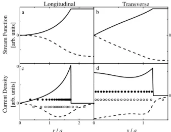
FIG. 1: Optimized stream functions (a and b) and optimal current densities (c and d) as a function of distance for longitudinal (a and c) and transverse (b and d) coils with biplanar geometry. Solid and dashed lines are the optimized primary and shielding distributions, respectively. Solid and open circles are the layouts of the optimal primary and shielding coils, respectively.
III. RESULTS
A C-language program, which computes Eq. (1) to (11), was developed to optimize the stream functions. Only 6 adjustable parameters were used for each stream function (Eqs.(3) and (4)). The Biot-Savart calculation of the gradient field [Eq. (11)] was performed over a grid of 16 points, uni-formly spaced in a square ROI (0<x<0.6a, 0<z<0.6a) in they=0 plane.
TABLE I: Parameters of the optimized stream functions. For longitudinal coilb=1.143a. For transverse coilb=1.2aandL=5.714a, and l=1.257a
Coil ε1 ε2 ε3 ε4 ε5 ε6 ε7 ηa2 L/a
[µT m/A] [mH/m] Longitudinal 0.850 4.357 1.740 0.000 0.913 0.000 0.183 3.246 0.989 Transverse 0.962 -0.058 -0.155 -0.080 0.223 -0.051 0.000 1.110 1.713
TABLE II: Magnetic field and electrical properties corresponding to shielded biplanar gradient coils. N = 18 (36) copper wires with 0.5 mm diameter were used in each primary plane, for longitudinal (transverse) coils.a= 3.5 cm.
Coil b z-HGVx-HGV η L R κ
[cm] [cm] [cm] [mT/m/A] [µH] [Ω] [%] Long.
Maxwell pair NS 3.08 3.84 8.88 186 0.8 Unshielded 3rd
Order [1] 4.15 2.14 3.24 4.64 157 1.0 91.56 Ref. [2] 4.00 5.16 4.22 2.12 32 1.3 95.26 This work 4.00 5.08 5.28 2.45 28 1.5 91.44 Tran.
Ref. [7] 4.15 2.25 2.50 2.13 280 2.5 76.00 3rd
Order [1] 4.20 1.84 2.16 2.61 279 2.5 96.40 5th
Order [1] 4.20 3.08 4.20 0.82 187 2.5 90.70 Ref. [2] 4.15 4.20 4.20 0.89 60 2.5 92.00 This work 4.15 4.44 4.64 0.81 49 2.5 91.00
were used. For the transverse coil 40 turns were used in each plane.
The optimized stream function parameters are listed in Ta-ble 1; this taTa-ble also lists the gradient efficiency at the gradient
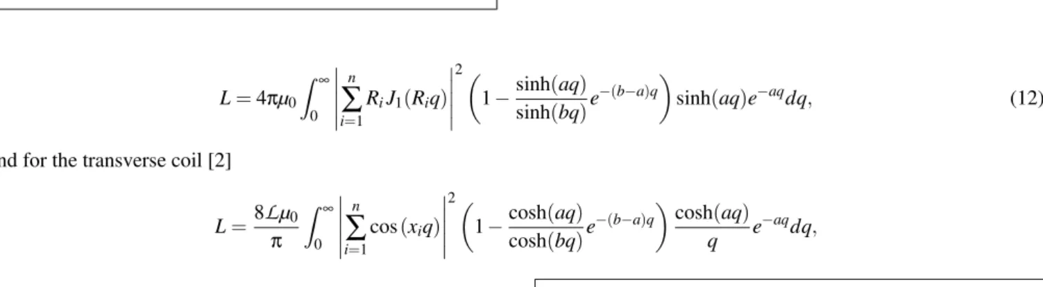
isocenter,η, and coil inductance,L, corresponding to the coils in Fig 1. Sinceηdecreases quadraticaly, andLincreases lin-early witha, values in Table 1 are generalized asηa2andL/a. For the longitudinal coil,Lwas evaluated by using [2]
L=4πµ0
Z ∞
0
¯ ¯ ¯ ¯ ¯
n
∑
i=1
RiJ1(Riq)
¯ ¯ ¯ ¯ ¯
2µ
1−sinh(aq)
sinh(bq)e
−(b−a)q
sinh(aq)e−aqdq, (12)
and for the transverse coil [2]
L=8
L
µ0 πZ ∞
0
¯ ¯ ¯ ¯ ¯
n
∑
i=1
cos(xiq)
¯ ¯ ¯ ¯ ¯
2
µ
1−cosh(aq)
cosh(bq)e
−(b−a)q
¶cosh(
aq)
q e
−aqdq,
was used. HereRiandxiare the positions of thei–wire in the longitudinal and transverse coils, respectively. These expres-sions includes self and mutual inductance between the wires in the primary and shielding planes.
Figure 2 shows the efficiency of the shielding coil to null the magnetic field in the outer region. These Biot-Savart calcula-tions were performed fora=0.035 m andz=0.05m. Solid lines are thez–component of the magnetic field produced by primary coils and dashed lines correspond to the field pro-duced by both primary and shielding coils in Fig 1. As shown in these figures, the shielding coils cancel at least 95% of the unshielded fields at this axial position (z=1.423a), which
0.00 0.01 0.02 0.03 0
1
Transverse
B
z[G/A]
x
[m]
0 1 2
0.00 0.01 0.02 0.03
Longitudinal
r
[m]
FIG. 2: Shielding performance as a function of distance, for the lon-gitudinal (top panel) and transverse (bottom panel) gradient coils. The curves are Biot-Savart calculations of the z-component of the magnetic field produced by the unshielded (primary plane; solid line), and shielded (primary and shielding planes; dashed lines) at z=5 cm.
-1.0 -0.5 0.0 0.5 1.0
-1.0 -0.5 0.0 0.5 1.0
Long Tran
z
/
a
x
/
a
FIG. 3: Contours of the 95% HGV produced by the gradient coils in the coronal plane. The solid (dashed) line corresponds to the longi-tudinal (transverse) design.
2, fora= 3.5 cm
The upper panels of Figs. 4 and 5 compare the layouts of the primary (solid circles) and shielding (solid triangles) coils proposed in Ref. [2] for the longitudinal and transverse gradi-ents, respectively, with those resulting from this method (open symbols). The optimized primary (solid line) and shielding (dashed line) stream functions used to get the wire positions are also shown in these figures. One advantage of the pro-posed method is related to the coil fabrication process. The coil layout corresponding to Ref. [2] is more difficult to ac-complish because of the shorter minimal distance between
neighbor wires. The present method uses smooth stream func-tions, which result in larger minimal gap between neighbor wires, facilitating coil construction.
0
0.00 0.07
Int. current density [arb. units]
r [m]
Primary
Shielding
Longitudinal gradient
0
0
Maxwell Ref. [12] This work
r
z
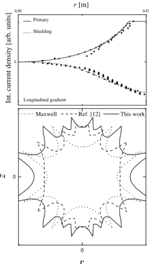
FIG. 4: [Top] Comparison of coil layouts resulting from the fast sim-ulated annealing method [2], and this work for the longitudinal gra-dient coil. The solid circles (triangles) are the wire positions in the primary (shielding) plane of ref [2]. The solid (dashed) line is the optimal stream function, and the open circles (triangles) are the wire positions in the primary (shielding) plane. [Bottom] Contours of the 95% HGV produced by the gradient coils in the coronal plane.
The bottom panels of Figs. 4 and 5 compare the limits of the 95% HGV produced by longitudinal and transverse gradient coils, respectively, in the coronal plane. Solid, dashed, and dotted lines correspond to the designs achieved in this work, Ref. [2], and Ref. [7], respectively. As shown in these figures, the optimization of stream functions results in coils producing larger HGV than those designed by our previous method [2].
IV. CONCLUSION
0
0.00 0.05
x[m]
Int. current density [arb. units]
Primary
Shielding
Transverse gradient
0
0
Ref. [15] Ref. [12] This work
x
z
FIG. 5: [Top] Comparison of coil layouts resulting from the fast simulated annealing method [2], and this work for the transverse gradient coil. The solid circles (triangles) are the wire positions in the primary (shielding) plane of ref [2]. The solid (dashed) lines is the optimal stream function, and the open circles (triangles) are the wire positions for the primary (shielding) plane in this work. [Bottom] Contours of the 95% HGV produced by the gradient coils in the coronal plane.
[1] E. C. Caparelli, D. Tomasi, and H. Panepucci, J. Magn. Reson. Imaging9, 725 (1999).
[2] D. Tomasi, E. C. Caparelli, H. Panepucci, and B. Foerster, Set. J. Magn. Reson.140, 325 (1999).
[3] K. Yoda, J. Appl. Phys.67, 4349 (1990).
[4] R. Turner, Magn. Reson. Imaging.11, 903 (1993).
[5] R. Bowtell, P. Mansfield, Minimum power, flat gradient pairs for NMR Microscopy - 8th ISMRM 1990.
[6] A. M. Peters, R. W. Bowtell, Magn. Reson. Materials in Physics, Biology, and Medicine,2, 387 (1994).
[7] V. Bangert, P. Mansfield, J. Phys. E: Sci Instrum. 15, 235 (1982).
[8] D. Tomasi, Magn. Reson. Med.45, 505 (2001).
[9] D. Tomasi. FSA design of a gradient coil set for head
imag-ing. Proceedings of the IV Mexican Symposium on Medical Physics, Juriquilla, Queretaro, M´exico, 2001. AIP Conference Proceedings593, 1 (2001).
[10] D. Tomasi, R.F. Xavier, B. Foerster, H. Panepucci, A. Tann ´us, and E.L. Vidoto. Magn. Reson. Med.48, 707 (2002).
[11] S. Crozier, D. M. Doddrell, J. Magn. Reson. A103, 354 (1993). [12] S. Crozier, L. K. Forbes, and D. M. Doddrell, J. Magn. Reson.
A107, 126 (1994).
[13] S. Crozier, D. M. Doddrell, Magn. Reson. Imaging13, 615 (1995).
[14] M. L. Buszko, M. F. Kempka, E. Szczesniak, D. C. Wang, and E. R. Andrew, J. Magn. Reson. B112, 207 (1996).
![FIG. 5: [Top] Comparison of coil layouts resulting from the fast simulated annealing method [2], and this work for the transverse gradient coil.](https://thumb-eu.123doks.com/thumbv2/123dok_br/18982175.457440/5.892.319.597.84.590/comparison-layouts-resulting-simulated-annealing-method-transverse-gradient.webp)
