The Lee-Yang Theory of Equilibrium and
Nonequilibrium Phase Transitions
R. A. Blythe
1and M. R. Evans
2 1Department of Physics and Astronomy, University of Manchester, Manchester M13 9PL, UK
2
School of Physics, University of Edinburgh, Mayfield Road, Edinburgh EH9 3JZ, UK
Received on 4 April, 2003
We present a pedagogical account of the Lee-Yang theory of equilibrium phase transitions and review recent advances in applying this theory to nonequilibrium systems. Through both general considerations and explicit studies of specific models, we show that the Lee-Yang approach can be used to locate and classify phase transitions in nonequilibrium steady states.
I
Introduction
In this work we seek a mathematical understanding of phase transitions in the steady state of stochastic many-body sys-tems. Systems at equilibrium with their environment pro-vide examples of such steady states, and the mechanisms un-derlying equilibrium phase transitions are long known and understood. Experimentally, one can distinguish between two types of transition: the first-order transition at which there is phase coexistence, e.g. between a high-density solid and a low-density fluid, and the continuous transition at which fluctuations and correlations grow to such an extent as to be macroscopically observable.
From a thermodynamical perspective, one can under-stand first-order transitions by associating with each phase a free energy. For a given set of external parameters, the phase ‘chosen’ by the system is that with the lowest free energy, and so a phase transition occurs when the free ener-gies of two (or more) phases are equal. The sudden changes in macroscopically measurable quantities that take place at first-order transitions are described mathematically as dis-continuities in the first derivative of the free energy. Discon-tinuities in higher derivatives relate to continuous (higher-order) phase transitions.
The tools of equilibrium statistical physics allow one— in principle at least—to express the free energy solely in terms of microscopic interactions. More specifically, the free energy is given by the logarithm of a partition
func-tion, a quantity that normalises the steady-state probability
distribution of microscopic configurations. Initially it was not universally accepted that this approach could faithfully describe phase transitions, in particular the first-order solid-fluid transition [1]. In order to show that the statistical me-chanical approach can reproduce the correct discontinuities in the free energy at a first-order transition, Lee and Yang [2] introduced a description of phase transitions concerning
zeros of the partition function when generalised to the com-plex plane of an intensive thermodynamic quantity. Initially, the theory was couched in terms of zeros in the complex fugacity plane which is appropriate for fluids in the grand canonical (fluctuating particle number) ensemble. However, by mapping a lattice gas onto the Ising model [3], the theory was found to hold equally well for a magnet in a fixed mag-netic field. Later [4-6] it became clear that the distribution of zeros in the complex temperature plane can reveal infor-mation about phase transitions in the canonical ensemble.
In section II we present a brief, self-contained discus-sion of the Lee-Yang theory of equilibrium phase transitions which relates nonanalytic behaviour in the free energy to ze-ros of the partition function. In the remainder of this article, we move our attention to phase transitions in
nonequilib-rium steady states, that is, those that carry currents of mass,
energy or some other quantity. We give therefore a very brief introduction to the established practice of modelling nonequilibrium physics through stochastic dynamics in sec-tion III. In particular, we will identify a candidate quantity for use in place of an equilibrium partition function when performing an Lee-Yang analysis of phase transitions. Fi-nally, in section IV we review recent work in which the Lee-Yang theory has been successfully applied to specific nonequilibrium phase transitions.
II
Overview of Lee-Yang theory of
equilibrium phase transitions
subject [2-6].
For concreteness we shall describe the theory in terms of a simple model system ofNspins in thermal contact with a heat reservoir. In this model system the energy of the sys-tem can take values E = nǫwithn = 0,1,2, . . . , M and the number of microstates corresponding to thenthenergy
level isg(n). The canonical partition function is given by ZN(β) =
M
X
n=0
g(n) exp(−βnǫ) (1) whereβis the inverse temperature. To investigate the zeros of this partition function, it is useful to make the change of variablez= e−βǫ. Then, the partition function is explicitly
a polynomial inzof degreeM and can be factorised as ZN(z) =
M
X
n=0
g(n)zn=κ
M
Y
n=1 µ
1−zz
n
. (2) Clearly the quantities zn are the M zeros of the partition
functionZN(z); meanwhile,κis a constant which we can
safely ignore in the following.
Since all theg(n)are positive, no zero ofZN(z)can be
real and positive: that is, the zerosznwill generally lie in the
complex plane away from the physical values ofzwhich lie on the positive real axis. We now define for all complexz
except the pointsz=znthe (complex) free energy
hN(z)≡
lnZN(z)
N . (3)
Using (2) we rewrite this as hN(z) = 1
N
M
X
n=1 ln
µ 1−zz
n
(4) and note that a Taylor series expansion of hN(z)around a
pointz6=znhas a finite radius of convergence given by the
distance to the nearest zero fromz. This then implies that thathN(z)can be differentiated infinitely many times over
any region of the complex plane that is devoid of partition function zeros. Since we identify a phase transition through a discontinuity in a derivative of the free energy, we see that such a transition can only occur at a pointz0in the complex
plane if there is at least one zero of the partition function ZN(z)within any arbitrarily small region around the point
z0.
Clearly this scenario is impossible if the number of zeros M is finite, except at the isolated pointszn where the free
energy exhibits a logarithmic singularity. Since such a point cannot lie on the positive real zaxis, there is no scope for a phase transition in a finite spin system, such as the sim-ple examsim-ple (1). On the other hand, if the partition function zeros accumulate towards a pointz0on the real axis as we
increase the number of spinsNto infinity there is the possi-bility of a phase transition.
In order to deal with the thermodynamic limit (see [8] for rigorous considerations) we shall assume that the limit
h(z) = lim
N→∞
lnZN(z)
N (5)
exists and we may write
h(z) = Z
dz′ρ(z′) ln³1− z
z′ ´
(6)
whereρ(z)is the local density of zeros in the complex-z plane in the thermodynamic limit.
Since the imaginary part of this complex free energy h(z)is multi-valued it will at times be more convenient to work with the potentialϕ(z)defined as
ϕ(z)≡Reh(z) = Z
dz′ρ(z′) ln¯¯ ¯1−
z z′ ¯ ¯
¯ . (7)
An expression for the densityρ(z)in terms of the poten-tialϕ(z)is easily obtained once one recognises thatln|z| is the Green function for the two-dimensional Laplacian. Specifically, ifz=x+iy, we have
∇2 ln|z| ≡
µ
∂2
∂x2 +
∂2
∂y2 
ln|x+iy|= 2πδ(x)δ(y).
(8) Using this expression, we can take the Laplacian of both sides of (7) to find
ρ(z) = 1 2π∇
2
ϕ(z). (9)
Such an equation is familiar from electrostatics and soϕ(z)
is analogous to an electrostatic potential.
In analogy to electrostatics, as long as we can integrate ρ(x)over bounded regions containing any singularities ofρ, the potential will be a continuous function [9]. The signifi-cance of this statement is that we can derive a rule for locat-ing phase boundaries given a partition function. Let us sup-pose that around pointsz1andz2in the complex plane, one
has (analytic) expressions for the potentialϕ1(z)andϕ2(z)
such thatϕ1(z)6≡ϕ2(z)(i.e. not the same function over the entirety of the complex plane). In order for the potential to be continuous at all points on the complex plane, we must have a phase boundary at those values ofz for which the condition
ϕ1(z) =ϕ2(z) (10) holds. This is basically the definition of a transition men-tioned above in the introduction. Sinceϕ1 andϕ2are
dif-ferent functions, some derivatives ofϕ(z)will not exist at these values ofzand we expect the density of zeros at these points to be non-zero. (It is also possible for zeros to be present at other points in the complex plane, but we do not need to consider this possibility here.)
Typically, a solution of (10) describes a curveCthat in-tersects the positive realzaxis at a pointz0. Having already
established that we require zeros to accumulate at the point z0in the thermodynamic limit for a physical phase transition
per unit length of this curve. We introduce the arclength swhich measures the distance alongCfrom the transition pointz0.
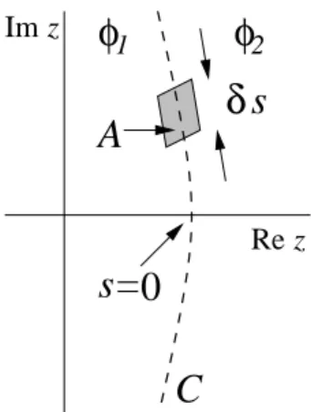
To obtain an expression for the line density of zerosµ(s)
along the curveC, consider a short section ofCof lengthδs enclosed by an areaAthat has two sides parallel toC and the other two sides perpendicular toC—see Fig. 1.
Integrat-ing the densityρ(z)over this area we have
Z
A
dzρ(z) =µ(s)δs . (11)
Meanwhile, we have from (9) and an application of the di-vergence theorem that
⌋
Z
A
dzρ(z) = 1 2π
Z
A
dz∇ ·[∇ϕ(z)] = δs
2π[∇ϕ2(z)− ∇ϕ1(z)]·nˆ (12) ⌈
in which the functionsϕ1(z)andϕ2(z)relate to the limiting values ofϕ(z)as the pointzon the curveCis approached from either side, and the vectornˆis the unit vector normal toCat that point.
z
Im
Re z
δ
s
s=0
φ
1φ
2C
A
Figure 1. Small areaAcovering a lengthδsof the curve of zerosC required to derive a relationship for the line densityµ(s)of zeros along the curve.
Recall thatϕ(z)is the real part of the complex free en-ergyh(z)and therefore, away from any zeros of the partition function, satisfies the Cauchy-Riemann equations
∂xϕ(z) =∂yψ(z) and ∂yϕ(z) =−∂xψ(z) (13)
in whichψ(z)is the imaginary part ofh(z)andz=x+iy. Then we have that
∇ϕ(z)·nˆ=∇ψ(z)·ˆt (14) whereˆtis the unit vector tangent to the curveCat the point z. Thus we recognise the scalar product in (12) as the di-rectional derivative of the imaginary part of the free energy
h(z)along the curveC. Putting this together with (11) we find that
µ(s) = 1 2π
d
ds[ψ2(z)−ψ1(z)] (15) in whichψ(z) = Im[h(z)]and the subscripts indicate oppo-site sides of a phase boundary.
Let us now assume that in the thermodynamic limit, there is a phase transition at the pointz0. Then, either side
of the transition the free energy can be written as
f1,2(˜z) =h(z0) +b1,2˜z+c1,2z˜2+. . . (16)
wherez˜=z−z0andf1(˜z)is valid forRe ˜z <0andf2(˜z)
valid forRe ˜z >0. Note that for the free energy to be real along the realzaxis, the coefficientsbandcmust also be real. From the criterion that the real part ofh(z)is continu-ous across a phase boundary, we find that the boundary lies along the curve
˜
y2 = ˜x2
+b2−b1
c2−c1 ˜
x (17)
wherex˜andy˜are the real and imaginary parts ofz˜ respec-tively. We consider the conditions under which a discon-tinuous (first order) or condiscon-tinuous (second or higher order) transition appear.
First-order transition
For the case whereb16=b2, and the free energy has a
discon-tinuity in its first derivative, the curve of zeros is a hyperbola that passes smoothly through the transition pointz0. Hence
the tangent to the curve of zeros is parallel to the imaginary axis atz0and using the rule (15) we find that
⌋
µ(0) = 1 2π
d
d˜y[(b2−b1)˜y+ 2(c2−c1)˜xy˜]
¯ ¯ ¯ ¯x˜= ˜y=0
= b2−b1
2π . (18)
Hence we see that the density of zeros at the transition point z0 is nonzero at a first-order phase transition (i.e. one at
which the first derivative of the free energy is discontinu-ous).
Second-order transition
Ifb1 =b2 butc2 6=c1we have that the curveCobeys the
equationy˜ =±x. Since the zeros of the partition function˜
come in complex-conjugate pairs, we find that the zeros ap-proach the pointz0along straight lines that meet at a
right-angle. If we consider the linex˜= ˜y =s/√2, we find from (15) that
µ(s) = 1 2π
d
ds(c2−c1)s
2
=c2−c1
π s . (19) This reveals that at a second-order phase transition, the den-sity of partition function zeros decreases linearly to zero at the phase transition point.
Higher-order transition
More generally, one can consider a difference in the free en-ergies either side of the transition point to have the leading behaviour f2(u)−f1(u) ∼ uα. Then the condition that
Re[f2(u)−f1(u)] = 0suggests that the curve of zeros ap-proaches the real axis at an angle 2πα. Unless α = 1, the curve does not pass smoothly through the real axis. In any case, the imaginary part of the free energy difference grows as|u|αgiving rise to a density of zeros that behaves assα−1
for small arclength s. This means that for the density of zeros to be finite at the transition point we must haveα≥1. In this section we have summarised what we refer to as the Lee-Yang theory of phase transitions. This describes how partition function zeros are related to phase transitions: the accumulation of zeros at a point along the physical (real, positive) axis of the control parameter gives the critical value and the density of zeros near to the accumulation point de-termines the order of the phase transition.
We derived a rule (10) for locating phase boundaries and a further rule (15) for finding the density of zeros along such boundaries. At a first-order transition there is a nonzero den-sity of zeros at the transition point whereas the denden-sity de-cays as a power-law to zero at the transition point when the associated phase transition is continuous.
Although we have discussed the theory of partition func-tion zeros with reference to the specific system described by the partition function (1) we should note that the ideas hold much more generally. Firstly, one is not restricted to the canonical ensemble: indeed in the original exposition of the theory [2], Lee and Yang worked in the grand canonical ensemble in which the quantity generalised to the complex plane was not a function of the temperature but rather the chemical potential. Of course, in the equilibrium theory, these intensive field-like quantities play similar mathemat-ical roles and so there is no reason why the Lee-Yang theory shouldn’t apply to all of them. For historical reasons, zeros in the complex fugacity (or chemical potential) plane are of-ten referred to as Lee-Yang zeros [2, 3] and those in the com-plex temperature plane Fisher zeros [4]. Also it appears that
one can just as easily generalise physical ‘field-like’ vari-ables (such as temperature) or ‘fugacity-like’ varivari-ables (such as the quantityz considered above) to the complex plane without altering the properties of the partition-function zero densities at first-order and continuous phase transitions de-scribed above.
Despite the apparently wide generality of the Lee-Yang theory of equilibrium phase transitions, proving its validity in the general case is a difficult task (although we note re-cent work in this direction [10]). Therefore, most rigorous results, such as those discussed in [8], tend to rely on spe-cific properties of a particular partition function. Perhaps the most spectacular of these is that obtained by Lee and Yang in their original work. Specifically, they found that the zeros of the partition function for an Ising ferromagnet in an external fieldhall lie on the circle|exp(h)| = 1. The significance of this result, which does not depend on the number of spa-tial dimensions, lattice structure and details of the spin-spin interactions, is that if there is a phase transition induced by varying the magnetic fieldh, it can only occur at the point h= 0, and then only if the partition function zeros accumu-late there in the thermodynamic limit.
III
Nonequilibrium steady states
A nonequilibrium steady state differs from its equilibrium counterpart in that it may admit a flow of, say, energy or mass. More generally, these states have a circulation of probability in the space of microscopic configurations. In the past few years, it has become customary to model nonequilibrium systems as stochastic processes, i.e. simple models defined by local dynamical rules. Extensive study of these has revealed a range of phenomena including nonequi-librium phase transitions [11-17]. We present below the key elements of this approach to nonequilibrium physics with a view to understanding nonequilibrium phase transitions in the framework of the Lee-Yang theory described above. In particular, we will need to propose a quantity to use in place of the equilibrium partition function (1).
Let us begin by discussing how one might realise the dynamics of the equilibrium spin system of the previous section, for example in a computer simulation. The aim is to generate a sequence of spin configurations such that the frequency with which a particular configuration C is generated is proportional to the Boltzmann weightf(C) = exp[−βE(C)]whereE(C)is the energy of configurationC. Usually this is achieved by choosing the next configuration C′ from the current configurationC with a probability
pro-portional to the transition rateW(C → C′)that satisfies the
detailed balance condition
f(C)W(C → C′) =f(C′)W(C′→ C) ∀ C,C′ . (20)
of any quantity in the steady state is zero (as it should be at equilibrium).
Since we are interested in nonequilibrium systems that support steady-state currents we must work with transition rates that do not satisfy the condition (20) or equivalent cri-teria (given in e.g. [19, 14, 17]). Clearly one has a lot of freedom in the choice of transition rates, and so in practice one often devises dynamics that seem physically reasonable given the phenomena one is trying to describe. Later, in sec-tion IV we will give concrete examples in the form of driven diffusive systems, in which particle moves are biased in a particular direction to model the effect of an external field.
In order to find the set of steady-state weights associ-ated with a particular set of prescribed transition rates, we impose the condition that the total flow of probability into a configurationCis balanced by the corresponding outflow. That is, we must have
X
C′6=C
[f(C′)W(C′ → C)−f(C)W(C → C′)] = 0 (21)
for every configurationC. In general there might be more than one solution to this set of equations for the weights f(C), each corresponding to a steady state that is reached with some probability that depends on the starting configu-ration. We shall assume for simplicity that the steady state is unique and therefore reached with certainty from every initial state. A sufficient condition for a unique steady state is that it is possible to reach each configuration from every other via a sequence of microscopic transitions [17].
Once the steady state weightsf(C)are known from (21) one can obtain the corresponding probability distribution of microscopic configurationsP(C)through a normalisation
Z =X
C
f(C) (22)
such that P(C) = f(C)/Z. Then, one can compute av-erages of physical quantities and look for nonanalyticities to locate nonequilibrium phase transitions as one varies the transition rates. At equilibrium we saw that the zeros of the function (1) that normalises the Boltzmann weights encodes the phase behaviour of the system. Thus we might hope that more generally, the zeros of the normalisation (22) will pro-vide information about nonequilibrium phase behaviour.
In section IV we review recent work that suggests that the steady-state phase behaviour of certain nonequilibrium driven diffusive and reaction-diffusion systems is correctly described by the zeros of the normalisation Z. Although we are unaware of any rigorous argument for this to be the case, some suggestive evidence is provided by an observa-tion made in [20, 17] which we now outline.
First note that the equation (21) is linear in the weights f(C). This implies that these weights, and hence the nor-malisation, can always be written as sums of products of the transition ratesW(C → C′). Now, by numbering the
micro-scopic configurations, one can construct the transition rate matrixW whose off-diagonal elements Wnm are equal to
the transition rates from configurationmtonand the diag-onal elementsWnn are negative and express the total rate
of departure from configuration n. Using elementary re-sults from matrix theory (see [20, 17] for the details), one can show that an expression for the normalisationZ that is polynomial in the transition ratesW(C → C′)is
Z = Y
λi6=0
(−λi) (23)
in whichλiare the eigenvalues of the matrixW.
With each of the eigenvaluesλi is associated an
eigen-vector ofW describing a ‘mode’ of the stochastic process that decays exponentially with a timescale τi = 1/|λi|
[17]. We have assumed that the process described by W has only one steady state, and so only one of the eigenval-ues is equal to zero (since clearly the relaxation time of a steady state is infinite). Equation (23) states that the nor-malisationZ can be written as a product of the remaining eigenvalues. Now, at a phase transition we expect diverg-ing timescales: physically one encounters metastable (long-lived) states near first-order transition points [21] and long correlation lengths and times at continuous transitions. The presence of long timescalesτi implies small eigenvaluesλi
of Wand, from (23), that the normalisationZ approaches zero. Hence it appears that it is appropriate to consider the zeros ofZas given by (22) to locate nonequilibrium phase transitions.
IV
Application of Lee-Yang theory to
nonequilibrium phase transitions
We shall now review recent progress in applying the Lee-Yang theory to nonequilibrium phase transitions. We con-sider first in section IV.1 driven diffusive systems, where most work has so far been focussed [21-23]. An appealing feature, discussed in more detail below, is that some one-dimensional cases have been solved exactly, the normalisa-tion (23) calculated, and nonequilibrium phase transinormalisa-tions analysed. (The existence of one-dimensional phase transi-tions contrasts with the case of one-dimensional equilibrium models which do not admit phase transitions if the interac-tions are short-ranged.) Then in section IV.2 we move onto reaction-diffusion systems and directed percolation. We do not endeavour to describe all possible nonequilibrium dy-namics in the following — for example, self-organised criti-cality has also been studied using a Lee-Yang approach [25].
IV.1 Driven diffusive systems
lattice site, so there is a hard-core exclusion in the lattice gas.
As discussed in section III, one can realise the dynamics of the lattice gas through a set of transition rates that sat-isfy the detailed balance condition (20) with respect to the Boltzmann distribution. Thirty years after Lee and Yang’s work, Katz, Lebowitz and Spohn (KLS) [26, 27] introduced a driven lattice gas model in which the rate at which particles hop in the direction of an external field is enhanced and the hop-rate against the field is suppressed. This model is well-studied and many results are discussed in [28]. The princi-pal effect of the driving field is to introduce anisotropy in the phase-separation that occurs below the critical temperature associated with the spontaneous magnetisation of the Ising ferromagnet (J >0) in two or more spatial dimensions and in the critical exponents that characterise this transition.
As yet, the KLS model remains unsolved for general interaction strength, although in one dimension the steady state is known for some parameters [29]. The particular case of one dimension and zero interaction strengthJ = 0, known as the asymmetric simple exclusion process (ASEP), had already been studied—at least at a mean-field level—by biophysicists interested in the kinetics of biopolymerisation
[30]. The mean-field approach predicts phase transitions in the steady state as parameters controlling the rate of inser-tion and extracinser-tion of particles at the boundaries are varied [31]. The existence of these phase transitions is confirmed through an exact solution of the ASEP [29-31], achieved using a powerful matrix product approach [32, 34] which has subsequently been used to solve many generalisations of the ASEP. The details of the matrix product method are not necessary for the following—suffice to say that one ends up calculating a normalisation proportional to (23) through a product of matrices, often of infinite dimension. In this way one obtains some explicit formulas for the normalisa-tion (22) which we shall use below1.
The asymmetric exclusion process with open boundaries is perhaps the simplest exactly solved nonequilibrium model that exhibits both a first-order and continuous phase transi-tion in its steady state. Therefore it is an ideal candidate for testing the hypothesis outlined in section III that zeros of the normalisation should accumulate towards the positive real axis in the complex plane of transition rates. Before outlining the results of this analysis (the details of which are presented in [23]) we recall the definition of the ASEP with open boundaries.
β
1
1
1
α
N N−1 2
1
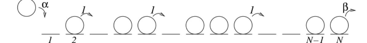
Figure 2. The dynamics defining the ASEP. The lattice is open and particles may be inserted or extracted at the boundaries as shown.
In this system, a particle on anN-site lattice can hop one site to the right at unit rate, as long as the receiving site is empty. Meanwhile, particles are inserted onto the leftmost lattice site (if empty) at a rateαand removed from the right-most site (if occupied) at a rateβ — see Fig. 2. Along the lineα=β < 1
2there is a coexistence between a high- and a
low-density phase, with a shock separating the two. This is
indicative of a first-order transition. Meanwhile, along the linesα > 1
2, β= 1
2 andβ > 1 2, α=
1
2there is a continuous
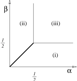
transition (i.e. one accompanied by diverging lengthscales) to a phase in which the particle current is independent ofα andβ. The phase diagram for the model is shown in Fig. 3.
The steady-state normalisation (22) for the ASEP with Nsites has been calculated [32] as
⌋
ZN(α, β) = N
X
p=1
p(2N−1−p)!
N!(N−p)!
(1/β)p+1
−(1/α)p+1
(1/β)−(1/α) . (24)
⌈
It is a simple matter to use a computer algebra package to solve this equation for its zeros in the complex-αplane at fixed N and β. (Equivalently, one could look at the complex-β zeros at fixedαsinceZN(α, β) = ZN(β, α).)
In Fig. 4 plots of the zeros are shown for β = 1, where a continuous transition occurs atα = 1
2, and forβ = 1 3,
where a first order transition occurs atα = 1
3. We
imme-diately notice that the curve of zeros seems to intersect the real positiveαaxis at the correct transition point. Further-more, the density of zeros near the first-order transition point (α = β = 1
3) seems to be uniform and nonzero, whereas
the density of zeros near the second-order transition point (α = 1
2, β = 1) seems to decrease to zero. Both of these
observations are in accord with the results known for equi-1
librium partition function zeros discussed in section II.
2 1
2
1
α
β
(ii)
(iii)
(i)
Figure 3. The phase diagram of the ASEP in the space spanned by the boundary ratesαandβ. The thick line represents a first-order phase boundary, the thin line a continuous phase boundary.
As shown in [23], the distribution of zeros in the ther-modynamic limit can be calculated once one knows that, for largeN, the normalisation behaves asZN ∼AJ−NNγ. In
this expression,A, Jandγdepend onαandβand the quan-tityJ is the current of particles across the lattice. Thus, the complex free energy (3) in the limitN→ ∞is
h(α, β) = lim
N→∞
lnZN(α, β)
N =−lnJ(α, β). (25) Furthermore for α smaller than the transition value αc,
J =α(1−α)whereas forα > αc,J =αc(1−αc).
Figure 4. Zeros of the normalisation in the ASEP in the complex-α plane andβ=1
3,1and lattice sizeN = 300.
Although an electostatic analogy was used in [23] to find the zero distribution, the mathematical content is the same as that used to derive the two rules (10) and (15) in sec-tion II. Applying the first rule, which demands that the real part of the free energy be continuous across a phase bound-ary, we find that the zeros ofZN(α, β)should lie along the
curve|α(1−α)| =αc(1−αc). It is therefore convenient
to change variable toξ=α(1−α). Then, in the complex-ξ plane, the zeros lie on the circle|ξ| = ξc = αc(1−αc).
The density of zeros on this circle can be found by setting ξ=reiθ and parametrising points on the circle ass=ξ
cθ.
Then, the second rule (15) gives the density of zerosµ(s)on the circle as
⌋
µ(s) = 1 2π
d
ds[Im lnξ−Im lnξc] =
1 2πξc
d dθθ=
1 2πξc
. (26)
⌈
That is, in the complex-ξ plane the zeros should become evenly distributed on a circle in the thermodynamic limit. Transforming the zeros of (24) obtained at different system sizes to the complex-ξplane reveals this to be the case [23]. Finally, one can show that near the intersection point between the curve of zeros in the complex-α plane and the positive real αaxis, the zeros of (24) sit on the curve x= 1
2 −(y 2+1
4−ξc)
1/2 wherexandyare the real and
imaginary parts ofα. For the caseβ < 1 2,ξc <
1 4 and the
transition is first order. One finds that the curve of zeros is smooth at the transition pointα=β, and that the density of zeros is(1−2β)/[2πβ(1−β)]which is nonzero. These are precisely the properties of the equilibrium partition function zeros at a first-order transition point (see section II).
At the continuous transition point (β ≥ 1
2 andξ = 1 4),
the zeros pass through the realαaxis along the line x = 1
2− |y|. Recall from section II that a transition ofn th
order has the curve of zeros meeting the positive real axis at an
angle of 2πn. Here the zeros clearly approach at an angleπ4 suggesting a second-order transition. In fact, one finds the density of zeros is π4sat a distancesalong this line, con-firming that the transition is second-order.
In summary, we have found that the Lee-Yang theory of first-order and continuous phase transitions applies to the normalisation of the nonequilibrium asymmetric exclusion process just as it does to the partition function of equilib-rium systems. Of course, this does not prove that the theory is generally applicable, and so there is some value in investi-gating other nonequilibrium steady states that exhibit phase transitions.
One such state is that initially studied by Arndt, Heinzel and Rittenberg [35, 36]. This model comprises M+ (M−)
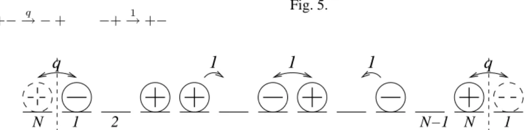
should two oppositely charged particles be next to one an-other, the following transitions can occur
+−→ −q + −+→1 +−
where the label above the arrow indicates the rate at which the transitions occur. These dynamics are illustrated in Fig. 5.
1
q
q
1
1
2
1 N−1 N 1
N
Figure 5. The dynamics defining the AHR model: labels indicate the rates at which the hops denoted by arrows can occur. Note that the N-site lattice is periodic.
Although a matrix product solution for this model is known to exist [36], it is technically difficult to work out the solution in its full generality [37]. However in the case of either a single vacancy [38] or a single negative particle, i.e. M− = 1[39] the steady-state normalisation is known
expl-citly and phase transitions have been identified. In the case M−= 1the zeros of the partition function in the complex-q
plane have been studied [24] and, once again the continuous phase transition present in this model is correctly described by the Lee-Yang theory.
A slightly different Lee-Yang analysis, that precedes the work described above, has been used to study the nonequi-lbrium phase transition that occurs at a finite density of va-cancies [22]. The motivation behind this study arose from computer simulations of the model [35, 36] for the case where the numbers of positive and negative particles were equal. In these simulations, three phases were initially iden-tified: a ‘solid’ phase for smallq, a ‘fluid’ phase for largeq and a mixed phase comprising the background ‘fluid’ and a large mobile droplet in an intermediate regime1 < q < qc
whereqcis some density-dependent quantity.
The steady-state normalisation ZN,M for the case of
M+ = M− = M positive and negative particles on the
N-site ring is not known exactly (at least in the canonical ensemble), therefore Arndt [22] chose to study the generat-ing function
ZN(z, q) =
X
M
zMZN,M(q) (27)
in the complex-zplane. Physically this approach is equiva-lent to placing the ring with nonequilibrium interactions in chemical equilibrium with a particle reservoir at fixed fu-gacity z. One can check that as one takes the thermody-namic limit, the relative size of the fluctuations in the den-sityr = M/N vanish, and so working at fixed fugacityz is equivalent to working at fixed densityr. (In fact, this is a standard ‘trick’ for dealing with closed systems in which the particle number is conserved, see e.g. [40].)
The key point here, however, is thatzis an equilibrium fugacity, and not a microscopic transition rate, and so the Lee-Yang theory of phase transitions described in section II
ought to apply directly here, without reference to the dis-cussion of section III. It was found [22] that whenq < qc
the zeros of (27) in the complex-zplane appear to lie along ellipses, intersecting the positive real axis. Conversely, for largerq the zeros appear to describe hyperbolæ that avoid the positive real axis. After investigating numerically the density of zeros in the complex-z plane, Arndt concluded that there is a fluid-fluid phase transition at some density-dependent pointqc>1.
Unfortunately, an exact asymptotic (i.e. largeN) analy-sis of the generating function (27) shows that the only non-analyticity occurs at the solid-fluid transition pointq = 1
[37]. However it was noted that physical quantities vary rapidly, but continuously, at some pointq > 1. This phe-nomenon has been explained as an abrupt increase in a cor-relation length to an anomalously large, but finite value [41]. We believe that resolution with the study of Arndt lies in the fact that the system sizes considered in [22] were quite small (N ≤100), whereas it was suggested [37] that the distinc-tion between this crossover behaviour and a genuine phase transition might become apparant only onceN is increased above about1070(an unfeasibly huge number!).
It would be interesting, therefore, to extend the numer-ical computation of zeros performed in [22] to much larger systems, to see how the ellipses noted above develop. For example it might well happen that instead of approaching the positive-real fugacity axis, the zeros of (27) would ter-minate a short distance away from it.
IV.2 Reaction-diffusion systems and directed percolation
A large and important class of models with stochas-tic dynamics is provided by reaction-diffusion systems2. In contrast to driven diffusive systems, where the particle-particle interactions imply conservation of particles, reaction-diffusion systems are characterised by dynamics that result in a change in particle number. Moreover there are a number of such systems that have absorbing states i.e. special configurations generally devoid of particles that once entered cannot be left. Phase transitions associated with 2
whether the system has a finite probability of not being ab-sorbed into such a state fall within the directed percolation and related universality classes [13]. We shall shortly dis-cuss the second order phase transition associated with the directed percolation university class in a little detail. Mean-while as a simple example of a reaction-diffusion system, we review a model for which the steady state that can be solved using the matrix product approach. The approach again pro-vides us with an explicit expression for the normalisation (22) by virtue of which we can analyse its zeros in the plane of complex reaction rates.
The system in question [42] has for the dynamics at neighbouring bulk sites on a one-dimensional lattice the pro-cesses
◦• → •◦q •◦ q→−1 ◦• •• → •◦q •• q→−1 ◦• ◦• → ••κq •◦ κq→−1 ••
occurring at the rates indicated, and with •representing a particle and◦an empty lattice site. It was demonstrated [42] that the matrix product scheme used for the ASEP could be generalised to cater for the steady state of the present reaction-diffusion system on a lattice ofNsites with reflect-ing boundary conditions (i.e. which is neither periodic nor has particle input or removal at the boundaries).
In the matrix product approach, the normalisationZN is
given by a scalar derived fromCN whereCis a square
ma-trix. IfCis a finite dimensionalm×mmatrix and can be diagonalised, the resulting expression forZN has the form
ZN(q, κ) = m
X
n=1
anλNn (28)
in whichλn is thenth eigenvalue ofCand the coefficients
an arise from the details of the way in which one obtains
a scalar from the matrixCN. A normalisation of this form
leads to a complex free energy h(q, κ) = lnhmax
n {λn}
i
(29) in which the maximum means the eigenvalue with the largest absolute value. Then, there is the possibility of a phase boundary when the magnitude of the two largest eigenvalues ofC are equal. It turns out that for the closed reaction-diffusion system introduced above,Cis a4×4 ma-trix that can be diagonalised whenq2
6
= 1 +κ[42]. When q2 = 1 +κ,C cannot be diagonalised on account of the
largest eigenvalue being degenerate, and a phase transition is found to occur at this point. Note that this scenario contrasts with the transfer-matrix approach to one-dimensional equi-librium systems where the partition function is also written as a product of matrices. Since all elements of the transfer matrix are positive the largest eigenvalue cannot become de-generate and therefore there can be no phase transition [12]. However there is no such restriction on the elements ofC, and so eigenvalue crossing is permitted and nonequilibrium one-dimensional phase transitions can occur.
The structure of the normalisationZN(q, κ)is even
sim-pler in the case where particles are inserted onto and re-moved from the left boundary at ratesαandβ respectively (with the right boundary remaining reflecting), and these rates satisfy the relationα=κ(q−1
−q+β)[43]. In this caseCis a2×2matrix and, forq2
6
= 1+κ, is diagonalisable with eigenvalues
λ1= 1 +κ and λ2=q 2
. (30)
We see then immediately from (29) and an application of the rule (10) that there is a phase boundary in the complexq plane along the circle|q|=√1 +κ. Also, since one of the eigenvalues does not depend on q, the free energyh(q, κ)
is a constant in one of the phases which, as the analysis of the normalisation zeros for the ASEP demonstrated, implies that the density of zeros on this circle is constant in the ther-modynamic limit. In turn, this implies that the phase transi-tion is first order, as confirmed by explicitly calculating the density profile in the two phases [43].
We finally turn our attention to a process that comprises symmetric decoagulation (that is, •◦ → ••and◦• → •• taking place with equal probability in each direction) and spontaneous decay (• → ◦) occurring at independent rates. Introduced as a crude model of an epidemic [44], this
con-tact process is known to exhibit a transition from a phase in
which the absorbing state (empty lattice) is reached with cer-tainty to a phase in which there is some probability that the epidemic remains active forever in the thermodynamic (in-finite system size) limit [45]. This transition occurs as the ratio between the decoagulation and decay rates is increased beyond a critical value.
n=0
n=3
n=4
n=5
n=6 n=1
n=2
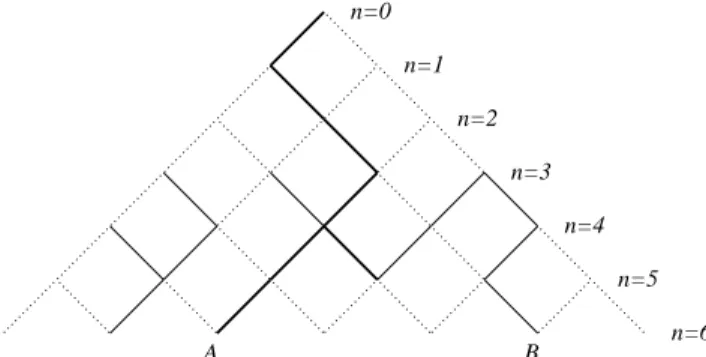
A B
Figure 6. Directed percolation. Bonds are open (solid lines) with probabilitypand closed (broken lines) with probability1−p. A
fluid starts at layern= 0and may flow only downwards through open bonds. Bonds carrying the fluid are shown with thick lines, so that the pointAon layern= 6is connected to the origin whereas pointBis not.
site. The fluid is allowed to flow along a bond pointing diag-onally downwards and then only if it is open. Each bond has a probabilitypof being open (and hence a probability1−p of being blocked), and the state of each bond is independent of any other and may not change with time.
The main quantity of interest in this system is the per-colation probability Pn(p) that the fluid can penetrate to
a depth n in the medium (see Fig. 6), averaged over all possible bond configurations. The order parameter for the model is the probabilityP∞(p)that the fluid can penetrate
infinitely far given a bond probabilityp. Ifpis below some critical percolation threshold pc, the fluid only ever
pene-trates a finite distance—i.e. a layer becomes dry with cer-tainty. However, for largerp, the order parameter becomes nonzero, growing asP∞(p) ∼ |p−pc|β withβ ≈ 0.276
near the critical point. The importance of the DP transition is that a wide range of models that have a transition into an absorbing state are expected to have that transition charac-terised by the DP exponents, one of which isβ[13]. Despite a huge amount of interest in directed percolation, none of the
models expected to belong to its universality class has been solved exactly.
Recently an attempt has been made to shed further light on the DP transition by studying the zeros of the percolation probabilityPn(p)[47, 48]. At first glance, a connection
be-tween this probability and a partition function is not obvious. However, associating with each site a ‘spin’ stateσi, that is
up if siteiis connected to a point on thenthlayer and down
otherwise, yields a form forPn(p)that has the structure of a
transfer-matrix representation of a partition function for an equilibrium system with three-spin interactions [49].
It is not clear that being able to givePn(p)the
appear-ance of a partition function necessarily implies that the Lee-Yang theory should hold. In particular,Pn(p)has some
fea-tures that set it apart from ‘standard’ equilibrium partition functions, in that it does not grow exponentially in the num-ber of bondsN, at least in the range0 ≤p≤1. It is also uncertain whether a free energy can meaningfully be defined for this system, especially in the region0≤p≤pcin which
limn→∞Pn(p) = 0.
pc 1
0 2 3
−1
Re(p) −0.75
−0.25 0.25 0.75
Im(p)
t=15 t=14 t=13 t=12 t=11 t=10 t=9 t=8
critical point
Figure 7. Zeros of the percolation probability on the directed percolation lattice up to depthsn= 15. Taken from [48] in which the symbol tis used where we usen.
Given these observations, it is perhaps not surprising that the zeros ofPn(p)calculated numerically forn≤15
(lead-ing to polynomials of degree up toN = 240) have a more complicated distribution than for the (exactly solved) mod-els considered so far. As is evident from Fig. 7, which was presented in [48], the zeros do not lie along a single curve but along a sequence of curves meeting at the critical point (as well as inside some region that encloses part of the real axis forp >2).
By considering the sequences of zeros approaching the positive real axis, one can estimate the critical pointpcand
dis-tributions than equilibrium steady states.
V
Summary and outlook
In this work we have revisited the Lee-Yang description of equilbrium phase transitions with a view to seeing whether the ideas apply to more general nonequilibrium transitions. Recently there have been a number of studies of zeros of partition-function-like quantities that arise in systems with nonequilibrium dynamics, and we have seen in our review of these works that the Lee-Yang theory, as described in sec-tion II, seems to hold quite generally.
We have argued that for dynamic models with a unique steady state, the normalisation defined as a sum over the steady-state configurational weights (22) serves as a suitable ‘partition function’ in the sense that its zeros, in the com-plex plane of any model parameter, should accumulate to-wards physical transition points in the thermodynamic limit. Furthermore, the density of zeros and angle of approach to the real axis indicate whether the transition is first-order (manifested physically through phase-coexistence) or con-tinuous (i.e. characterised by divergent correlation lengths and times). Thus studying the zeros of the normalisation (22) provides an unambiguous classification of nonequilib-rium phase transitions as do the Lee-Yang zeros in the equi-librium case.
The observation that backs up this scenario is embod-ied by equation (23) which reveals that the reciprocal of the steady-state normalisation is equal to the product of the characteristic relaxation times in the dynamics. Since near a phase transition one expects timescales to diverge, one also expects the normalisation to approach zero. However, a rig-orous argument for this to be the case is still lacking. More-over (23) implies a possible link between systems for which the steady state normalisation can be calculated and those for which eigenvalues of the transition matrix can in princi-ple be calculated.
A different class of systems encompasses those whose steady state is not unique. The contact process is, in fact, an example of such a model, in which the absorbing state is reached with certainty below the critical decoagulation rate, whereas above it, and on an infinite system, a second steady state can also be reached with some nonzero proba-bility. Since this additional steady state exists only when the lattice size becomes infinite, one must take that limit first, before taking time to infinity. Otherwise, on a finite sys-tem the steady state is simply the absorbing state and the steady-state normalisation is trivially equal to a constant. Nevertheless the work of [47, 48], which we reviewed in section IV.2, indicates that the Lee-Yang theory can be rele-vant when one considers other properties of the nonequilib-rium system such as the percolation probability.
Although we have not discussed this in great detail here, it should be noted that the Lee-Yang approach gives a method for extrapolating to the thermodynamic limit from solutions for small system sizes. In the work of [48],
nu-merical solutions for small systems were used successfully to estimate the transition point and density of zeros as it is approached. From this information one learns about the na-ture of the phase transition and, for example, can estimate the values of critical exponents. This is a common technique in equilibrium statistical physics (see e.g. [50]) and it may be the case that stochastic processes unyielding to analytical treatment could be understood this way.
Acknowledgments
We thank Bernard Derrida for helpful discussions. R.A.B. acknowledges financial support under EPSRC grant GR/R53197.
References
[1] C. Domb, The critical point: a historical introduction to the
modern theory of critical phenomena (Taylor & Francis,
Lon-don, 1996).
[2] C. N. Yang and T. D. Lee, Phys. Rev. 87, 404 (1952). [3] T. D. Lee and C. N. Yang, Phys. Rev. 87, 410 (1952). [4] M. E. Fisher, The nature of critical points, in Lectures in
Theoretical Physics, edited by W. E. Brittin, volume 7C, p. 1
(University of Colorado Press, Boulder, 1965).
[5] S. Grossmann and W. Rosenhauer, Z. Physik 218, 437 (1969). [6] S. Grossmann and V. Lehmann, Z. Physik 218, 449 (1969). [7] L. E. Reichl, A Modern Course in Statistical Physics
(Uni-versity of Texas Press, Austin, 1980).
[8] D. Ruelle, Statistical Mechanics: Rigorous Results (W A Benjamin, New York, 1969).
[9] O. D. Kellogg, Foundations of Potential Theory (Dover, New York, 1953).
[10] M. Biskup, C. Borgs, J. T. Chayes, L. J. Kleinwaks, and R. Koteck´y, Phys. Rev. Lett. 84, 4794 (2000).
[11] J. Marro and R. Dickman, Nonequilibrium Phase Transitions
in Lattice Models (Cambridge University Press, Cambridge,
1999).
[12] M. R. Evans, Braz. J. Phys. 30, 42 (2000). [13] H. Hinrichsen, Adv. Phys. 49, 815 (2000).
[14] D. Mukamel, Phase Transitions in Nonequilibrium Systems, in Soft and Fragile Matter, edited by M. E. Cates and
M. R. Evans, Vol.53 of Scottish Universities Summer School
in Physics, p. 237 (Institute of Physics Publishing, Bristol,
2000).
[15] G. M. Sch¨utz, Exactly Solvable Models for Many-Body Sys-tems Far From Equilibrium, in Phase Transitions and
Crit-ical Phenomena, edited by C. Domb and J. L. Lebowitz,
Vol. 19, p. 1 (Academic Press, London, 2001). [16] R. Stinchcombe, Adv. Phys. 50, 431 (2001).
[17] M. R. Evans and R. A. Blythe, Physica A 313, 110 (2002). [18] O. Narayan and A. P. Young, Phys. Rev. E 64, 021104 (2001). [19] N. G. van Kampen, Stochastic processes in physics and
[20] R. A. Blythe, Nonequilibrium Phase Transitions and
Dynam-ical Scaling Regimes. Ph.D. thesis, University of Edinburgh
(2001). http://www.ph.ed.ac.uk/cmatter/links/rab-thesis. [21] B. Gaveau and L. S. Schulman, J. Math. Phys. 39, 1517
(1998).
[22] P. F. Arndt, Phys. Rev. Lett. 84, 814 (2000).
[23] R. A. Blythe and M. R. Evans, Phys. Rev. Lett. 89, 080601 (2002).
[24] F. H. Jafarpour, J. Phys. A: Math. Gen. 36, 7497 (2003). [25] B. Cessac and J. L. Meunier, Phys. Rev. E 65 036131 (2002). [26] S. Katz, J. L. Lebowitz, and H. Spohn, Phys. Rev. B 28, 1655
(1983).
[27] S. Katz, J. L. Lebowitz, and H. Spohn, J. Stat. Phys 34, 497 (1984).
[28] B. Schmittmann and R. K. P. Zia, Statistical Mechanics of
Driven Diffusive Systems, Vol. 17 of Phase Transitions and Critical Phenomena (Academic Press, London, 1995).
[29] J. Krug and H. Spohn, Kinetic Roughening of Growing Sur-faces, in Solids Far From Equilibrium, edited by C. Godr`eche (Cambridge University Press, Cambridge, 1992).
[30] C. T. MacDonald, J. H. Gibbs, and A. C. Pipkin, Biopolymers
6, 1 (1968).
[31] B. Derrida, E. Domany, and D. Mukamel, J. Stat. Phys. 69, 667 (1992).
[32] B. Derrida, M. R. Evans, V. Hakim, and V. Pasquier, J. Phys. A: Math. Gen. 26, 1493 (1993).
[33] G. Sch¨utz and E. Domany, J. Stat. Phys. 72, 277 (1993). [34] B. Derrida, Phys. Rep. 301, 65 (1998).
[35] P. F. Arndt, T. Heinzel, and V. Rittenberg, J. Phys. A: Math. Gen. 31, L45 (1998).
[36] P. F. Arndt, T. Heinzel, and V. Rittenberg, J. Stat. Phys. 97, 1 (1999).
[37] N. Rajewsky, T. Sasamoto, and E. R. Speer, Physica A 279, 123 (2000).
[38] T. Sasamoto, Phys. Rev. E 61, 4980 (2000).
[39] F. H. Jafarpour, J. Phys. A: Math. Gen. 33, 8673 (2000). [40] B. Derrida, S. A. Janowsky, J. L. Lebowitz, and E. R. Speer,
J. Stat. Phys. 73, 813 (1993).
[41] Y. Kafri, E. Levine, D. Mukamel, and J. Torok, J. Phys. A: Math. Gen. 35, L459 (2002).
[42] H. Hinrichsen, S. Sandow, and I. Peschel, J. Phys. A: Math. Gen. 29, 2643 (1996).
[43] F. H. Jafarpour, J. Phys. A: Math. Gen. 36, 7497 (2003). [44] T. E. Harris, Ann. Prob. 2, 969 (1974).
[45] D. Griffeath, Additive and Cancellative Interacting Particle
Systems, Vol. 724 of Lecture Notes in Mathematics
(Springer-Verlag, Berlin, 1979).
[46] S. R. Broadbent and J. M. Hammersley, Proc. Camb. Phil. Soc. 53, 629 (1957).
[47] P. F. Arndt, S. R. Dahmen, and H. Hinrichsen, Physica A 295, 128 (2001).
[48] S. M. Dammer, S. R. Dahmen, and H. Hinrichsen J. Phys. A: Math. Gen. 35, 4527 (2002).
[49] R. J. Baxter and A. J. Guttmann, J. Phys. A: Math. Gen. 21, 3193 (1988).
[50] W. Janke and R. Kenna, Nucl. Phys. B Proc. Supp. 106, 905 (2002). See also hep-lat/0112032.
[51] S. Redner, Scaling Theories of Diffusion-Controlled and Ballistically-Controlled Bimolecular Reactions, in
Nonequi-librium Statistical Mechanics in One Dimension, edited by