ISSN-1697-1523 eISSN-1139-3394 DOI:10.3369/tethys.2010.7.03 Journal edited by
ACAM
Analysis of a method for radar rainfall estimation considering
the freezing level height
R. Bordoy1,2, J. Bech1, T. Rigo1and N. Pineda1 1Servei Meteorol`ogic de Catalunya, Berl´ın 38, 08021 Barcelona
2Department of Astronomy and Meteorology, Universitat de Barcelona, Mart´ı i Franqu´es 1, E-08028 Barcelona
Received: 12-III-2009 – Accepted: 4-VIII-2009 –Translated version
Correspondence to:[email protected]
Abstract
Quantitative precipitation estimation provided by weather radars plays a vital role in many hydrometeorological applications. The complexity of all the factors that contribute, on the one hand, to rainfall processes, and on the other hand, to the behavior of the energy beam emitted by the radar in its traverse through the atmosphere, mean that current estimates generally dif-fer from the precipitation observed on surface. The aim of this study was to validate the SRI product (Surface Rain Intensity), which is a method of radar rainfall estimation that applies a correction considering a vertical profile of reflectivity (VPR). The VPR takes into account the freezing level height to make a correction in areas affected by the phenomenon known as “bright band”. Precipitation estimates obtained through this method were compared with other methods currently operational in the Meteorological Service of Catalonia in five representative episodes of convective and stratiform rainfall. In general, better results were obtained when compared with raingauge observations. Although this is a preliminary assessment that will have to be com-pleted with more case studies, the results indicate good prospects for an operational use of this method.
Key words:VPR correction, bright band, quantitative precipitation estimate, meteorological radar
1 Introduction
There is increasing interest in getting good estimates of precipitation at ground level by using remote sensing tools. As hydrometeorological models and short-term prediction systems improve, it becomes necessary to have a rainfall field in almost real time that covers all the area being considered. Rain gauges, despite being the paradigmatic instru-ments for measuring precipitation, are generally inadequate for hydrometeorological applications (Collier, 1986). Since they only allow measuring isolated precipitation values, it is difficult to obtain a continuous field of measurements cov-ering the whole territory, especially in areas of complex to-pography (Germann et al., 2006). The meteorological radar, however, makes it possible to obtain a rainfall field in al-most real time for areas up to 250 km of radius, although further than 100 km the quality of the estimate is usually very reduced (Joss and Waldvogel, 1990). It is therefore an
indispensable instrument in terms of displaying and track-ing precipitattrack-ing structures and it makes possible, together with a hydrological model, to issue warnings of possible flash floods and mitigate both personal and material damage.
However, it is important to consider that the measure-ments taken by the radar are subjected to various sources of error. These can be grouped into three categories (Zawadzki, 1984; Joss and Lee, 1995; Dinku et al., 2002):
• Errors caused by the radar system itself (bad electronic calibration, errors in the orientation of the antenna). • Errors related to the interaction between the radar wave
and the environment (ground clutter, animals, airplanes, orographic blocking, echoes in clear air, rain attenua-tion, increase of the beam volume with distance). • Errors in converting the reflectivity radar measurements
Figure 1. Location of the 4 operative radars of the radar network of the Meteorological Service of Catalonia: LMI, CDV, PBE and PDA. The radar used is the one that appears as CDV. The points indicate the location of the available rain gauges: the black ones are the ones used in this study and the blue ones are omitted (as later explained in this article).
or relationZ −R, non-uniform vertical profile reflec-tivity (PVR)).
Given normal propagation conditions and the subse-quent curvature of the microwave beam emitted by the radar, the beam height increases with distance from the radar. The impact of this effect is that the precipitation detected by the radar can be located at altitudes far above the ground, and therefore, effects such as the bright band (Cunningham, 1947; Vignal et al., 2000), orographic enhancement (Brown-ing, 1980; Cotton et al., 1983) or evaporation, among oth-ers, provoke that the algorithms applied directly to the re-flectivity value measured by the radar at a certain height pro-vide accumulation values that may be very different from those registered by the rain gauges in the area at ground level.
The bright band effect plays a key role in these errors. The bright band is a layer where the reflectivity detected by the radar is strongly increased. The reason for this phe-nomenon is the following: when solid hydrometeors parti-cles cross the melting layer they begin to melt and are cov-ered by a thin layer of liquid water. The radar interprets them as very large drops of liquid precipitate and the reflectivity values may be increased up to a factor of about 7 dB. This increase occurs due to the fact that solid and liquid precipi-tation have different dielectric constants and different speeds of falling, which makes the reflectivity values detected by the radar different depending on the stage of precipitation (Rine-hart, 1997).
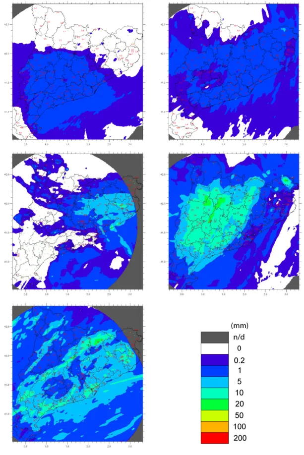
Table 1.Maximum precipitation accumulation values in 1 h and in 24 h as estimated by the radar for the different episodes considered.
Date Maximum 24-hour
precipitation in 1 h (mm) accumulation (mm)
02/01/08 5.0 10.9
03/01/08 27.7 48.6
22/03/08 20.4 46.6
20/04/08 18.6 66.4
12/07/08 47.6 64.2
The first corrections applied to radar measurements were based primarily on climatic corrections depending on the area of the precipitation (Collier, 1986). Corrections from the VPR were first suggested by Koistinen (1991), who thought that if it was possible to determine the change of reflectivity according to height, the value measured by the radar up to the surface could be extrapolated and therefore provide a much more accurate result. This theory, although encouraging, is limited by the difficulty in measuring the VPR and its rapid variation with time and space. Although different approaches have been proposed to determine it (An-drieu and Creutin, 1995; Vignal et al., 1998; Mittermaier and Illingworth, 2003), the most effective way to make this cor-rection has not been established yet.
This article is structured as follows: the methodology section presents the study area, the technical characteristics of the radar used, the analyzed configurations of the SRI product and the statistics for the analysis. This is followed with showing the results, and the article closes with a brief discussion about the conclusions reached.
2 Methodology
The study area has been Catalonia, which is located in the northeast of the Iberian Peninsula, characterized by a complex topography and directly influenced by the Mediter-ranean Sea (Figure 1). In order to evaluate the product in question the radar located in la Panadella (41.6◦N, 1.4◦E, 825 m) was used. It is a Doppler radar that operates in C band (5,600 to 5,650 MHz) and is part of the Radar Network of the Meteorological Service of Catalonia (Servei Meteorol`ogic de Catalunya, hereafter, SMC) (Bech et al., 2008). This radar performs 16 scans between 0.6◦and 27◦per 6 minutes, and a Doppler filter is applied to remove fixed echoes. The reso-lution of the data is 1 km and 1◦.
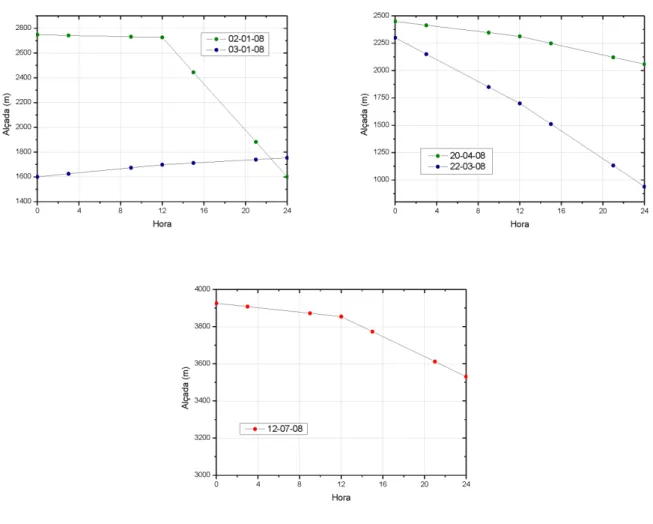
Figure 3.Temporal evolution of the freezing level height on the study days: a) (upper left) winter episodes, b) (upper right) spring episodes, c) (bottom) summer episode. The X axis contains hours and the Y axis height.
The analyzed product, called SRI (Surface Rain Inten-sity) is based on a methodology of VPR correction developed by the Finnish meteorological service (Koistinen, 1991) and is part of the IRIS software (Interactive Radar Information System), from the radar manufacturer Vaisala Sigmet (Sig-met, 2006). IRIS is a software that makes it possible to pro-gram the acquisition of data and generate derived products with a weather radar. Among the different products of IRIS (PPI, RHI, CAPPI...), SRI allows a correction in the vertical profile of reflectivity and therefore minimizes the bright band effect.
SRI performs an extrapolation of the reflectivity value obtained by the radar at the lowest height where precipita-tion is detected all the way to the ground level. This process is carried out following a theoretical vertical profile of reflec-tivity previously defined in the product configuration phase (Figure 4). The typical correction values are between -10 dB and +5 dB depending on the height of the freezing level, the distance to the radar and the lowest elevation angle of the an-tenna (in mm h−1
a factor 4 is reached due to the logarithmic
nature of the relationship between reflectivity and precipita-tion intensity).
Knowing the type of precipitation is crucial when de-ciding what type of correction should be applied. If it is a convective precipitation, the bright band effect does not oc-cur or, in specific cases, it is very weak (Fabry and Zawadzki, 1994). Therefore, in the case of convective precipitation the SRI does not extrapolate the value detected by the radar fol-lowing the theoretical VPR (Figure 4), but instead modifies it by assigning the convective pixel the precipitation value of the lowest pixel without clutter (non precipitating echoes) that is located in its vertical and considers VPR to be constant all the way to the surface. However, in case of stratiform pre-cipitation, the SRI corrects the reflectivity value detected by the radar through the theoretical VPR shown in Figure 4.
Figure 4. Representation of the profile of reflectivity (VPR) used by the SRI product in case of stratiform precipitation in order to make the VPR correction. A0 refers to the freezing level height and therefore the beginning of the bright band;ARto the reference height where the extrapolation would be made.Siis the reflectivity
gradient where ice predominates (over the bright band). D repre-sents the width of the bright band andIits intensity.Srrepresents
the reflectivity gradient due to rain, under the bright band.
Table 2.Values of the monthly climatic average height of the freez-ing level recommended for middle latitudes in the SRI product (Sig-met, 2006).
Month Freezing level height (km)
January 1.0 February 1.0 March 1.5 April 2.0 May 2.5 June 3.0 July 3.5 August 3.5 September 3.0 October 2.5 November 1.5 December 1.0
considered in this parameter was the value used by the SRI by default (7 dBZ km−1). Regions 2 and 3 are within the bright band. This area is characterized by a sudden increase of the reflectivity that later decreases. This effect appears due to the presence of a mixture of liquid and solid precipi-tation and due to the interaction of the energy beam emitted by the radar with this mixture (Collier, 1986). The parame-ters involved in these regions are the thickness of the melting layer (by default D=1 km) and the intensity of the peak of the melting layer (by default I=7 dBZ). Below the melting layer,
in region 1, the gradient of the reflectivity is given by “Sr” (1 dBZ km−1
). This last gradient of reflectivity is considered in order to take into account the reinforcement of the precip-itation due to orographic reasons.
In the set up phase of the product, the parameters of the vertical profile of reflectivity can be selected. In this way the most appropriate profile possible can be adjusted, based on the characteristics of the precipitation and the location. In ad-dition to the parameters discussed in section 2.1, we can also choose whether the extrapolation will be made to sea level or to the surface given by a digital elevation model (DEM). An automatic distinction between convective and stratiform precipitation can also be activated.
From here on the SRI settings will be discussed. Each setting uses a theoretical VPR with a different bright band height. We should point out the importance of not confus-ing the real freezconfus-ing level with the freezconfus-ing level used by the SRI product when making the extrapolation; the closest the corrections are to the real theoretical freezing level, the more accurate the corrections will be.
The following SRI settings were analyzed for each episode:
• SRI-DEM, SRI-withoutDEM: these two settings have been made from the freezing level heights provided by the sounding data of Barcelona. As there are only two data points per day (00h and 12h), a linear interpolation was performed to know, in an initial approximation, the values of the freezing level’s height at 6h, 9h, 15h, 18h and 21h. From these two values, two settings were gen-erated: the SRI-DEM, which applies the correction to the surface given by the digital elevation model, and the SRI-without DEM, which applies the correction to sea level.
• SRI-Extremes: two extreme cases have been included here regarding the height of the freezing level. In one of them, the freezing level height was taken at 0 m and in the other case at 4500 m. From this point forward they will be called SRI-0m and SRI-4500m respectively. The interest of studying these two configurations is to eval-uate the response of the product to the two extreme ex-trapolations: taking the gradient of reflectivity above the bright band (freezing level to 0 m) or below it (freezing level to 4500 m).
• SRI-climates: named as such because it consists of 12 individual settings. Each of them takes the height of the climatic freezing level per month for mid-latitudes (see Table 2).
In all cases the relationZ−Ris the one used by Mar-shall and Palmer (1948):
Z= 200R1.6 (1)
whereZ (mm6 m−3
) is the reflectivity andR (mm h−1 ) is the intensity of the precipitation.
Figure 5.Temporal evolution of the hourly average bias of the SRI-DEM and operative CAPPI products for the days: a) 22.3.07, b)12.7.08, c) 2.1.08 and d) 3.1.08. The sections without data of figure b) are caused by the absence of precipitation in those hours.
(e.g. Ulbrich and Lee, 1998), it has been decided to fix it for all cases in order to focus the study on the influence of the vertical profile of reflectivity in the estimation of precipita-tion, thus avoiding the introduction of more degrees of free-dom.
To perform automatic discrimination between convec-tive and stratiform precipitation, the SRI product uses a cri-terion applied in the original study by Koistinen (1991). Specifically, the precipitation is considered to be convective if the value of reflectivity is over 34 dBZ or if there is pre-cipitation at 2 km above the freezing level. Although there are studies that show that non-convective precipitation can be found over 34 dBZ (Rigo and Llasat, 2004), this value was chosen because it is the value used by the SRI by default; fu-ture studies can analyze the implications of its variation. For other methods to distinguish between different types of pre-cipitation, see as an example S´anchez-Diezma (2001), Rigo and Llasat (2004) or Bech et al. (2005).
In addition to comparing the different SRI configura-tions to each other, we also considered the operative
prod-ucts for precipitation estimation using radar at the SMC. On the one hand, we studied the precipitation obtained with the lower CAPPIs (Constant Altitude Plan Position Indicator), at 1 km height (CAPPI products are obtained by making a hor-izontal cut of the radar data interpolated at the same height). The CAPPI product also uses theZ −R Marshall-Palmer relation and only corrects the estimates by eliminating fixed echoes with a Doppler filter.
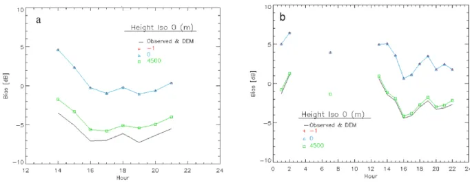
Figure 6. Temporal evolution of the hourly average bias of the SRI-extremes products for the episodes of the days: a) 02.1.08 and b) 12.7.08. The sections without data of figure b) are caused by the absence of precipitation in those hours.
In order to evaluate the merits of the various radar prod-ucts analyzed, their measurements were compared with the values recorded by the rain gauges of the network of auto-matic meteorological stations of the SMC (Prohom and Her-rero, 2008). It was considered fitting to select the rain gauges located at distances under 100 km of the radar in order to avoid errors caused by the increase of the volume of the radar beam at a distance. Similarly, with respect to the radar, the ones that presented an orographic blocking lesser than 10% were chosen. This selection led to the usage of 81 rain gauges out of a total of 161 available rain gauges (see Figure 1). The study was carried out using hourly and 24-hour accumula-tions, comparing rain accumulations with the precipitation integrations of the pixel that occupies the position of the rain gauge. Rain gauge measurements greater than 0.5 mm with a radar estimate larger than 0.2 mm were considered to be valid.
The statistical indexes used to evaluate the different products related with the rain gauges are the following: the biasB, measured in dB, that makes it possible to find the dif-ference of the average values between a radar estimate and a rain gauge estimate:
B =10
N N X
i
10 logPradar(i)
Ppluvio(i)
(2)
the average squared error (RMSE), measured in mm, in order to evaluate the magnitude of the average error between both samples. The use of the normalized square root of the differ-ences prevents cancellations that can occur when getting, at times, positive difference values and in other cases negative difference values:
RM SE=
v u u t1
N N X
i
[Pradar(i)−Ppluvio(i)]2 (3)
Figure 7.Representation of the VPR considered for positive freez-ing level heights (thick dark curve) and the VPR considered for freezing level heights under 0 m SRI-0m (fine grey curve). The ice (Si) and rain (Sr) VPR slopes are indicated; the intermediate peak, that begins under the freezing level (in this case at 2200 m), corresponds to the bright band with a thickness of 1000 m. The ar-row shows that at low levels -where most rain gauges are located-the reflectivity value registered by located-the SRI-0m exceeds located-the observed one and, therefore, produces an overestimate. The abcisas axis rep-resents the growing reflectivity to the right and the ordinate axis represents height.
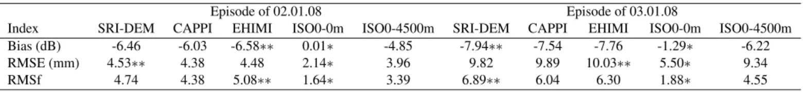
Table 3. Summary of the statistical products for the winter episodes. Minimum values are indicated with the symbol “∗” and maximum
values with “∗∗”.
Episode of 02.01.08 Episode of 03.01.08
Index SRI-DEM CAPPI EHIMI ISO0-0m ISO0-4500m SRI-DEM CAPPI EHIMI ISO0-0m ISO0-4500m Bias (dB) -6.46 -6.03 -6.58∗∗ 0.01∗ -4.85 -7.94∗∗ -7.54 -7.76 -1.29∗ -6.22
RMSE (mm) 4.53∗∗ 4.38 4.48 2.14∗ 3.96 9.82 9.89 10.03∗∗ 5.50∗ 9.34
RMSf 4.74 4.38 5.08∗∗ 1.64∗ 3.39 6.89∗∗ 6.04 6.30 1.88∗ 4.55
Figure 8.Image of the reflectivity (scale in dBZ) obtained with the radar from la Panadella on 2 January 2008 at 17:30 Z. A gradient of precipitation intensity with an approximately circular symmetry is appreciated, which indicates the presence of bright band. The time of this observation corresponds to the hour of the secondary peak in the representations of the temporal evolution of the average bias of this episode.
RM Sf = exp
v u u t1
N N X
i
ln
Pradar(i) Ppluvio(i)
2
(4)
whereNis the number of valid precipitation data,Ppluvio(i) refers to the hourly/24-hour accumulation in the rain gaugei (mm) and Pradar(i)to the hourly/24-hour accumulation by the radar in the position of the rain gaugei(mm).
The analyses carried out and their importance for the evaluation of the studied product have been organized as fol-lowing:
• Carrying out a study of the temporal evolution of the average bias in order to see if the sample is very biased and/or if there are marked variations of its value over time.
• Studying the bias distribution in relation with the dis-tance in order to investigate whether its behavior fol-lows the same pattern in all different products and dif-ferent episodes.
• Representing the frequency distribution of the bias for the hourly and 24-hour values in order to determine the dispersion and homogeneity of the sample and, conse-quently, the consistency of the analyzed product. • Creating scatter diagrams with the main products
(CAPPI, EHIMI and SRI-DEM). These diagrams rep-resented, on the one hand, all hourly values of precipi-tation, and on the other hand all the 24-hour accumula-tion values. This way, by using an adjustment for square minima the average bias and the linearity of the sample can be qualitatively and quantitatively visualized. • Analyzing the indexes discussed in the previous
sec-tion in order to have quantitative results and to compare them with other works that have been published on the same theme.
3 Results
This section presents a selection of results for each episode based on the previous list.
3.1 Temporal evolution of the average bias
3.1.1 SRI-DEM regarding CAPPI
In three of the five episodes analyzed, the SRI-DEM product was less biased with regard to the rain gauges than the CAPPI, except at some specific hours (Figures 5a, 5b and 5d). Regarding the other episodes, the estimates made by CAPPI are slightly less biased than the ones by SRI-DEM (Figure 5c).
3.1.2 SRI-extremes
Figure 9. Temporal evolution of the hourly average bias of the SRI-climatic products for the days: a) 2.1.08 and b) 20.4.08. There are 12 months and only 6 curves. The months with the same climatic height as the freezing level are in the same color.
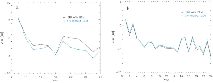
Figure 10.Temporal evolution of the hourly average bias of the SRI-DEM and SRI-without DEM products for the days: a) 22.3.08 and b) 20.4.08.
width of a bright band of about 1 km, the VPR slope corre-sponding to the height of the largest part of the rain gauges (between 0 and 1000 m) corresponds to liquid precipitation. On the other hand, the SRI-0m slope corresponds to solid precipitation, which causes the estimated values to be over-estimation (Figure 7). As the freezing level becomes lower, it goes from an overestimate to underestimate. Figure 8 shows the increase in reflectivity caused by the bright band effect (clear ring structure around the radar) at the hour when there is a slight increase of the overestimate by the SRI-0m.
In the summer convective episode (Figure 6b), the SRI-4500m together with the SRI-DEM get the least bi-ased results. The fact that throughout the episode both SRI-DEM and the SRI-4500m get the same average bias values, and therefore of estimated precipitation, shows that
the leakage by convective rain of the SRI product works properly.
Figure 6 also represents the estimate if the freezing level is below sea level, called “-1”. In this case the extrapolation is entirely performed using the gradient of reflectivity of re-gion 4, considering all the solid precipitation. For the studied area, as the whole surface is above sea level, the results are identical as in the case of SRI-0m. However, for places such as the Netherlands, where part of its land is below sea level, this option is highly relevant.
3.1.3 SRI-climatic
freez-Figure 11.Distribution of the 24-hour average bias for the day 2.1.08: a) SRI-DEM, SRI-0m and SRI-4500m products and b) SRI-without DEM, CAPPI and EHIMI products for the day 20.4.08. c) SRI-DEM, SRI-0m and SRI-4500m products and d) SRI-without DEM, CAPPI and EHIMI products. The lines indicate the average eased value of the symbols in the same color.
ing level of the months that coincide with the month of the episode (e.g. Figure 9a). For the case of 20 April 2008 (Fig-ure 9b), the month that minimizes the bias is May instead of April. This fact is associated with the fact that on that day the freezing level height was higher than the climatic average in April.
3.1.4 SRI-DEM regarding SRI-withoutDEM
After analyzing the various episodes considered, it was verified that the implementation of a DEM in the SRI prod-uct does not vary the estimate of precipitation excessively (Figure 10). However, the extrapolation down to the surface given by a digital terrain model does not increase the bias in any of the cases, and it is therefore always advisable to implement it in order to get the most accurate estimates of precipitation possible.
3.2 Distribution of bias with distance
Figure 12. Histograms of the average bias for 24-hour accumulations of 2.1.08: a) SRI-DEM, SRI-0m and SRI-4500m products and b) SRI-DEM, CAPPI and EHIMI products, and of 12.7.08: c) SRI-DEM, SRI-0m and SRI-4500m products and d) SRI-DEM, CAPPI and EHIMI products.
3.3 Quantitative Analysis
Tables 3 to 5 show the average values for each episode of the statistical indexes evaluated in this study. For purposes of clarity the minimum values are indicated with the symbol “∗” and the maximum with “∗∗”.
Although it is worth noting that the gentle curve may lead to erroneous conclusions, it should be interpreted only as a trend and not as an absolute value of the bias regarding the distance. The use of symbols is necessary for absolute values.
3.4 Histograms of the bias
Performing these types of representations, has made it possible to see the dispersion of the bias values for 24-hour accumulations and therefore evaluate the consistency of the studied products. All products were found to be consistent with the default settings, that is to say, the dispersion of their bias values is small. It is observed that in the winter cases
the less biased setting is again the one that implements the freezing level at 0 m, showing a very focused peak at 0 dB and a maximum frequency value of 25 values (Figure 12a). In comparison with Figure 12b, it shows that the SRI-0m is the one that obtains less biased estimates, also with regard to SRI-DEM, CAPPI and EHIMI.
In the summer convective case the less biased settings have been those that used the freezing level at 4500 m (Fig-ure 12c). Compared with the operating products, the SRI-DEM shows a more pronounced and centered peak at 0 dB than the CAPPI or the EHIMI (Figure 12d).
3.5 Scatter diagrams
Table 4. Summary of the statistical products of the spring episodes. Minimum values are indicated with the symbol “∗” and maximum
values with “∗∗”.
Episode of 22.03.08 Episode of 20.04.08
Index SRI-DEM CAPPI EHIMI ISO0-0m ISO0-4500m SRI-DEM CAPPI EHIMI ISO0-0m ISO0-4500m Bias (dB) -0.57∗ -3.83∗∗ -3.07 3.04 -2.61 -3.61 -2.76 -3.69∗∗ 3.44 -1.93∗
RMSE (mm) 3.41∗ 5.06 4.93 13.88∗∗ 3.84 9.91 8.59 9.57 23.65∗∗ 7.52∗
RMSf 1.96∗ 2.85∗∗ 2.41 2.62 2.33 2.54 2.14 2.58∗∗ 2.54 1.90∗
Table 5. Summary of the statistical products of the summer episode of 12.7.08. Minimum values are indicated with the symbol “∗” and
maximum values with “∗∗”.
Index SRI-DEM CAPPI EHIMI ISO0-0m ISO0-4500m Bias (dB) -1.77 -2.66 -4.44∗∗ 3.64 -1.44∗
RMSE (mm) 8.18 8.97 11.01 28.69∗∗ 7.94∗
RMSf 2.01 2.26 3.52∗∗ 2.81 1.94∗
line; a slope above the diagonal shows an underestimate of the radar in relation with the rain gauges, while the opposite situation shows an overestimate of the radar measurements. This analysis used the values of 24-hour accumulations for all cases. The number of points in the diagrams of Figure 13 indicate the number of valid points used in the calculation.
The case of 22 March 2008 shows how the correction of SRI-DEM (Figure 13a) does reduce the bias of both the CAPPI (Figure 13b) and the EHIMI (Figure 13c). However, the highest correlation is the one presented by the EHIMI system, with a value of 0.89, while the SRIDEM gets a low-est correlation, of 0.83. The CAPPI correlation is 0.87 and lies between the two previously discussed cases. As we can observe, the correlations are very high in the three cases, with the EHIMI product that gets the highest correlation in every case. A systematic underestimate was observed both with the CAPPI and the EHIMI, which could indicate a possible error in radar calibration. The same situation is observed in Figures 13d and 13f, where the underestimate slope of the SRI-DEM is lower (Figure 13d) while the larger correlation coefficient is the one of the EHIMI system (Figure 13f).
We can see that the configurations of the SRI product with the freezing level height at 0 presented the values with less error in the winter cases (Table 3), obtaining a bias of nearly 0 dB and very low RMSE and RMSf. The products with the highest errors in these cases are the SRI-DEM and the EHIMI.
In the spring cases (Table 4), the variability of the freez-ing level caused more dispersed results. The products that got the highest errors were the CAPPI and the EHIMI; how-ever, the fact that the SRI-0m product presented such a high RMSE shows that the value of its bias is not significant be-cause of the high number of cancellations, causing the result to be masked with a lower value than it should be.
In the case of the summer episode (Table 5) the result of the SRI-4500m is the most satisfactory, as it obtained a
bias of -1.44 dB. We can observe that the SRIDEM also ob-tains reasonable values, with a bias of -1.77 dB. In this case the SRI-0 and the EHIMI showed the greatest errors. Re-garding the SRI-0m, it obtained a RMSE of 28.69 mm, in-dicating that the absolute error was considerable and that the effect of the cancellations masked the bias again. On the other hand, the results of the EHIMI showed that its filter-ing softens the convective precipitation peaks in excess, and therefore, in such episodes, its precipitation measurement is quite underestimated.
For clarity and simplicity, the products that obtained lower RMSE and bias for each episode are marked in Ta-ble 6. It is confirmed that the different configurations of the SRI are those that got lower statistical errors in all cases.
4 Conclusions
Table 6.Products that carried out the estimation with the least bias and the least RMSE in each episode.
Episode CAPPI EHIMI SRI-DEM SRI-0m SRI-4500m
02-01-08 X
03-01-08 X
22-03-08 X
20-04-08 X
12-07-08 X X
(SRI-DEM) implemented does not get the best results in all episodes.
Focusing attention on the representations in which there is a comparison between SRI with observed freezing levels with and without DEM, we could see that, in such episodes, the usefulness of DEM is rather low. However, the results are always positive and therefore it is always recommendable to implement it. An important consideration for possible operative uses of the SRI product are the good results obtained with the SRI-climatic. Despite the fact that it estimates precipitation less carefully than the specific SRI for each episode, it is a good first approach to an operational use of the SRI product. However, in order to minimize statistical errors, the implementation of the height of the freezing level by meteorological output models is recommended. Doing this makes it possible to take into account, in a more effective way, freezing level variability and the VPR used in the extrapolation will be closer to the real one.
The precipitation estimates made with the CAPPI product are not the most accurate in any case; this confirms that in order to make quantitative estimates of precipitation it is really necessary to apply corrections to the values directly recorded by the radar.
When using the EHIMI system, estimation of precipita-tion is not the one with the least bias in any case. This result suggests that there may be some part within the EHIMI system that filters in excess, as the maximum precipitation values are excessively eased. However, we must add that in two of the five cases analyzed the value of the correlation coefficient R2
obtained by the EHIMI in the 24-hourly accumulations are the highest of the three products analyzed. This result could lead us to believe that possible errors in the radar calibration would have increased the errors obtained in the EHIMI estimate of precipitation, given its particular sensitivity to such problems.
The scatter diagrams of all episodes, confirm that the linearity of the estimated precipitation values regarding those observed by the rain gauges is generally higher in the 24-hour accumulations than in the hourly accumulations. This fact is caused by the strong irregularity of rainfall both in space and in time; so as the local observations are integrated, the values of the accumulations are increasingly homogeneous. This result, together with the histograms shown, that have a narrow base and high peaks in general,
bring us to the conclusion that the products analyzed are consistent with their respective configurations.
Another point in favor of the SRI product is its fast processing. The application of the correction takes longer than that generated by a CAPPI, and is therefore very im-portant for operational purposes. However, for operative use it would be suitable to implement more than two daily data of the freezing level height, for example using numerical model outputs as well.
At any rate, it must be clear that these results are preliminary. The correction of the vertical profile of reflec-tivity is subject to many variables that make it an extremely difficult and delicate task. Therefore, in order to increase the reliability of these conclusions it would be necessary, on the one hand, to carry out this study with other values of the theoretical VPR parameters that have remained invariable for all the cases, such as the intensity of the peak of the melting layer, its thickness or reflectivity gradients above and below the melting layer. Alternative values can be extracted from the bibliography, such as those used by the UK Met-Office (Scovell et al., 2008). On the other hand, it is necessary to add more precipitation episodes for each season to the study and see the evolution of the different products that are evaluated.
Acknowledgements. This study was conducted in the framework of the EU European concerted action COST-731 Propagation of Uncertainty in Advanced Hydro-meteorological Systems. The first author has benefited from a grant from the SMC during the years 2007-2008, during which most of this work was developed. We also appreciate the comments of Oriol Argem´ı (SMC) and two anony-mous reviewers who contributed to improve the final version of this work.
References
Andrieu, H. and Creutin, J. D., 1995:Identification of vertical pro-files of radar reflectivity for hydrological applications using an inverse method. Part I: Formulation, J Appl Meteorol,34, 240– 258.
Bech, J., Gjertsen, U., and Haase, G., 2007: Modelling weather radar beam propagation and topographical blockage at northern high latitudes, Q J R Meteorol Soc,133, 1191–1204.
Bech, J., Rigo, T., Pineda, N., Argem´ı, O., Bordoy, R., and Vi-laclara, E., 2008: An updated description of the radar network of the Meteorological Service of Catalonia, 5th Eur. Radar Conf. ERAD2008, Finland.
Browning, K. A., 1980: Structure, mechanism and prediction of orographically enhanced rain in Britain. Orographic Effects in Planetary Flows, World Meteorological Organization, 85-114. Collier, C. G., 1986:Accuracy of rainfall estimates by radar, Part 1:
Calibration by telemetering raingauges, J Hydrol,93, 207–223. Cotton, W. R., George, R. L., Wetzel, P. J., and McAnelly, R. L., 1983: A long-lived mesoscale convective complex. Part I: The
mountain-generated component, Mon Wea Rev, 111, 1983–
1918.
Cunningham, R. M., 1947: A different explanation of the “bright line”, Journal of Meteorology,4, 163.
Dinku, T., Anagnostou, E. N., and Borga, M., 2002: Improving radar-based estimation of rainfall over complex terrain, J Appl Meteorol,41, 1163–1178.
Fabry, F. and Zawadzki, I., 1994: Long-term radar observations of the melting layer of precipitation and their interpretation, J Atmos Sci,52, 838–851.
Franco, M., S´anchez-Diezma, R., and Sempere-Torres, D., 2006:
Improvements in weather radar rain rate estimates using a method for identifying the vertical profile of reflectivity from vol-ume radar scans, Meteorologische Zeitschrift,15, 521–536. Germann, U., Galli, G., Boscacci, M., and Bolliger, M., 2006:
Radar precipitation measurement in a mountainous region, Q J R Meteorol Soc,132, 1669–1692.
Gjertsen, U., Sˆalek, M., and Michelson, D. B., 2004:
Gauge-adjustment of radar-based precipitation estimates, COST Action 717, ISBN-92-898-0000-3.
Joss, J. and Lee, R., 1995: The application of radar-gauge com-parisons to operational precipitation profile corrections, J Appl Meteorol,34, 2612–2630.
Joss, J. and Waldvogel, A., 1990: Precipitation measurements and hydrology, Amer Meteorol Soc, Battan memorial and 40th an-niversary of the radar meteorology, pp. 577-606.
Koistinen, J., 1991: Operational correction of rainfall errors due to the vertical reflectivity profile, Amer Meteorol Soc, Preprints, 25th Int. Conf. on Radar Meteorology, Paris, France, 91-96. Marshall, J. and Palmer, W., 1948: The distribution of raindrops
with size, Journal of Meteorology,5, 165–166.
Mittermaier, M. and Illingworth, A., 2003: Comparison of model-derived and radar-observed freezing-level heights: Implications for vertical reflectivity profile-correction schemes, Q J R Meteo-rol Soc,129, 83–95.
Prohom, M. and Herrero, M., 2008: Cap a la creaci d’una base de dades climtica de Catalunya (segles XVIII a XXI), Tethys,5, 3–11.
Rigo, T. and Llasat, M. C., 2004:A methodology for the classifica-tion of convective structures using meteorological radar: Appli-cation to heavy rainfall events on the Mediterranean coast of the Iberian Peninsula, Nat Hazards Earth Syst Sci,4, 59–68. Rinehart, R. E., 1997: Radar for Meteorologists, Rinehart
Publica-tions, Grand Forks, USA, 428pp.
S´anchez-Diezma, R., 2001: Optimizaci´on de la medida de lluvia por radar meteorol´ogico para su aplicaci´on hidrol´ogica, PhD the-sis, Universitat Polit`ecnica de Catalunya.
S´anchez-Diezma, R., Sempere-Torres, D., Bech, J., and Velasco, E., 2002: Development of a hydrometeorological flood warning system (EHIMI) based on radar data, 2nd Eur. Radar Conf. Eu-ropean Meteorological Society. Copernicus Gesellschat, Delft, Holland.
Scovell, R., Lewis, H., Harrison, D., and Kitchen, M., 2008: Local vertical profile corrections using data from multiple scan eleva-tions, Proceedings 5th Eur. Radar Conf. ERAD2008, Finland. Sigmet, 2006: Iris Product and Display Manual. Chapter 2.14. SRI:
Surface Rainfall Intensity, Sigmet, Inc., Westford, Boston, MA, USA.
Ulbrich, C. W. and Lee, L. G., 1998: Rainfall measurement error by WSR-88D radars due to variations in Z-R law parameters and the radar constant, J Atmos Ocean Technol,16, 1017–1024. Vignal, B., Andrieu, H., and Creutin, J., 1998:Identification of
ver-tical profiles of reflectivity from volume scan radar data, J Appl Meteorol,38, 1214–1228.
Vignal, B., Galli, G., and Joss, J., 2000: Three methods to deter-mine profiles of reflectivity from volumetric radar data to correct precipitation, J Appl Meteorol,39, 1715–1726.