Making Sense of the Experimental Evidence on
Endogenous Timing in Duopoly Markets
†Luís Santos-Pinto
Universidade Nova de Lisboa, Departamento de Economia Campus de Campolide, PT-1099-032, Lisboa, Portugal
Email address: [email protected]
September 5, 2006
Abstract
The prediction of asymmetric equilibria with Stackelberg outcomes is clearly the most frequent result in the endogenous timing literature. Several experi-ments have tried to validate this prediction empirically, but failed tofind support for it. By contrast, the experimentsfind that simultaneous-move outcomes are modal and that behavior in endogenous timing games is quite heterogeneous. This paper generalizes Saloner’s (1987) and Hamilton and Slutsky’s (1990) en-dogenous timing games by assuming that players are averse to inequality in payoffs. We explore the theoretical implications of inequity aversion and com-pare them to the empirical evidence. Wefind that this explanation is able to organize most of the experimental evidence on endogenous timing games. How-ever, inequity aversion is not able to explain delay in Hamilton and Slutsky’s endogenous timing games.
JEL Classification Numbers: C72, D43, D63, L13.
Keywords: Endogenous Timing; Cournot; Stackelberg; Inequity Aversion.
†I gratefully acknowledgefinancial support from an INOVA grant. I am also thankful
1
Introduction
The theoretical literature on endogenous timing started with Saloner (1987), Hamilton and Slutsky (1990), and Robson (1990). This literature tries to iden-tify factors that might lead to the endogenous emergence of sequential or simul-taneous play in oligopolistic markets.
Saloner (1987) analyzes a duopoly with two periods wherefirms can produce inboth periods before the market clears. In thefirst periodfirms simultaneously choose initial production levels. The choices of thefirst period are observed and then additional non-negative second period outputs are chosen simultaneously. Saloner shows that if production costs are the same across both periods, then there is a continuum of equilibria: any point on the outer envelope of the reaction functions between thefirm’s Stackelberg outputs is attainable with a subgame perfect Nash equilibrium (SPNE). Additionally, in all of these equilibria pro-duction takes place only in the first period. However, Ellingsen (1995) shows that only the two Stackelberg equilibria in Saloner’s game survive elimination of weakly dominated strategies.1
In Hamilton and Slutsky (1990)’s action commitment game, twofirms must decide a quantity to be produced inoneof two periods before the market clears. If afirm commits to a quantity in thefirst period, it acts as the leader but it does not know whether the otherfirm has chosen to commit early or not. If a firm commits to a quantity in the second period, then it observes thefirst period production of the opponent (or its decision to wait). Hamilton and Slutsky show that this game has three SPNE: bothfirms committing in the first period to the simultaneous-move Cournot-Nash equilibrium quantities, and each waiting and the other playing its Stackelberg leader quantity in thefirst period. They also show that only the Stackelberg equilibria survive elimination of weakly dominated strategies.2
Observed behavior in experiments on these two canonical models of endoge-nous timing is at odds with the theory. For example, Huck et al. (2002) test experimentally the predictions of Hamilton and Slutsky (1990)’s action commitment game. They find that: (i) Stackelberg outcomes are rare, (ii) simultaneous-move Cournot outcomes are modal, (iii) simultaneous-move out-comes are often played in the second production period, and (iv) behavior is quite heterogeneous—in some cases followers punish leaders, in other cases col-lusive outcomes are played, and in other cases Stackelberg warfare is observed.3 Müller (2006) tests the predictions of Saloner’s game extended by Ellingson. He finds that: (i) Stackelberg outcomes are extremely rare, (ii) simultaneous-move 1Several papers have suggested ways to reduce the set of equilibria in Saloner’s model
by modifying the structure of the game. For example, Robson (1990) introduces discount-ing between periods, Pal (1991) introduces cost asymmetries between periods, Maggi (1996) introduces uncertainty about demand.
2A model where the price is chosen was considered by Robson (1990), and a Stackelberg
outcome is also obtained.
symmetric outcomes are the most frequent outcomes, (iii) sometimes collusive outcomes are observed, (iv) there is production in both periods with 84% of production taking place in thefirst period, (v) subjects seem to attempt to bal-ance market shares in the second production period, and (vi) subjects do not produce more than the Stackelberg follower’s quantity in thefirst production period.4
The questions that the endogenous timing literature tries to address are par-ticularly relevant in terms of new markets, where two or morefirms will enter. The experimental evidence suggests that simultaneous-move play may a better predictor of behavior in markets for new goods than sequential play.5 It also suggests that there may be substantial heterogeneity in behavior in these mar-kets. In some cases collusive outcomes may emerge, in other cases Stackelberg warfare, and in others still sequential play with Stackelberg like outcomes.6
Why does the theory perform poorly in the experiments? One possibility is that subjects are not able to iteratively rule out dominated strategies and stop after one or two rounds of reasoning. There is substantial experimental evidence that supports this view. Even if subjects are able to do eliminate dom-inated strategies the two Stackelberg equilibria involve large payoffdifferences and this creates a coordination problem. This implies that playing the Stack-elberg leader’s quantity is risky by comparison with playing the Cournot-Nash quantity.7
It is possible to think of explanations for some aspects of the empirical evidence. However, it is much harder to explain all of the experimentalfi nd-ings. For example, the risk-payoffequilibrium selection argument may explain why simultaneous-move outcomes are more frequently played than Stackelberg outcomes. However, it cannot explain the emergence of collusive outcomes or Stackelberg warfare. It is also not clear how this explanation can account for the fact that simultaneous-move play can take place in the second production period in Hamilton and Slutsky’s action commitment game.
The gap between the theory and the experimental evidence is the main mo-tivation behind this paper. To bridge this gap the paper assumes that players in endogenous timing games have social preferences. The paper derives the predictions of this explanation for both Saloner’s and Hamilton and Slutsky’s endogenous timing games and compares the predictions to the empirical evi-dence.
Social preferences have been shown to explain a broad range of data for many different games. The clearest evidence for these type of preferences comes from bargaining and trust games. For example, in ultimatum games offers are usually much more generous than predicted by equilibrium and low offers are
4Section 2 discusses the experimental evidence on endogenous timing games.
5As we have seen the prediction of Stackelberg equilibria rests on equilibrium selection
argumens. Simultaneous-move Cournot-Nash equilibria typically exist, however, they do not survive the application of equilibrium refinements.
6Bagwell (1995) points out that the theoretical prediction of Stackelberg outcomes
cru-cially depends on the perfect observability of the Stackelberg leader’s action. However, the experiments assume perfect observability which rules out this explanation.
often rejected. According to the social preferences explanation, these offers are consistent with an equilibrium in which players make offers knowing that other players may reject allocations that appear unfair. Huck et al. (2002), Müller (2006), and Fonseca et al. (2005b) suggest that inequity aversion may also explain behavior in endogenous timing games. However, these papers do not formalize this explanation.
The paper starts by generalizing Saloner’s (1987) game and Hamilton and Slutsky’s (1990) action commitment game by assuming that players are averse to inequality in payoffs. To incorporate inequity aversion in endogenous timing games we make use of Fehr and Schmidt’s (1999) approach. That is, we as-sume that an inequity averse player dislikes advantageous inequity—i.e. it feels compassion towards the opponent if the opponent has lower profits—and also dislikes disadvantageous inequity—i.e. it feels envy towards the opponent if the opponent has higher profits.
The paper shows that relatively high levels of inequity aversion rule out asymmetric equilibria in both Saloner’s game as well as in Hamilton and Slut-sky’s action commitment game. In other words, relatively high levels of inequity aversion favor simultaneous-move play over sequential play. The intuition for this result is straightforward. For relatively high levels of inequity aversion, playing leader type outcomes leads to inequity costs which are larger than the material benefits of leadership.8
The paper also shows that inequity aversion gives rise to a continuum of symmetric equilibria in both Saloner’s game as well as in Hamilton and Slutsky’s action commitment game. The intuition for this result is as follows. Suppose that a player knows that his opponent will produce the Cournot-Nash quantity. If this player is averse to inequity, then his best response is to produce also the Cournot-Nash quantity. Producing an output different from the Cournot-Nash quantity reduces the player’s material payoffand increases inequity costs. Now, suppose that a player knows that his opponent will produce somewhat less than the Cournot-Nash quantity. If this player is averse to advantageous inequity, then his best response is to produce exactly the same quantity as the opponent. Producing a higher quantity than the opponent increases the player’s material payoffby less than the cost from advantageous inequity. Similarly, if a player knows that his opponent will produce somewhat more than the Cournot-Nash quantity, then his best response is also to produce the same quantity as the opponent. Producing a lower quantity than the opponent increases the player’s material payoffby less than the cost from disadvantageous inequity.
The previous paragraph shows us that inequity aversion may lead both play-ers to produce less than the Cournot-Nash quantity. This happens whenever players have a relatively high level of compassion and are able to coordinate on a “collusive outcome.” Similarly, inequity aversion may lead both players to produce more than the Cournot-Nash quantity. This happens whenever play-ers have a relatively high level of envy and are unable to coordinate on the 8Relatively low levels of inequity aversion do not rule out asymmetric equilibria. In fact, as
Cournot-Nash equilibrium. Thus, if a population is composed of players with heterogeneous social preferences and these individuals are matched in pairs to play endogenous timing games, then heterogeneity in behavior is to be expected. It turns out that inequity aversion is able to explain most of the experi-mental evidence on Saloner’s game. As we have seen, inequity aversion can rule out asymmetric equilibria and generates a continuum of simultaneous-move symmetric equilibria. Inequity aversion can also explain the fact that subjects produce in both periods. This happens because inequity aversion gives rise to a multiplicity of symmetric equilibria in the game and subjects have to coordi-nate on one of them. If subjects are unable to coordicoordi-nate in one of the multiple symmetric equilibria in thefirst production period, then they have an incentive to produce in the second production period to attain coordination before the market clears. The lack of coordination on a symmetric outcome in thefirst period also explains why players act as if they wish to balance market shares in the second production period.
Inequity aversion is also able to explain most experimentalfindings on Hamil-ton and Slutsky’s action commitment game. Inequity aversion can rule out se-quential play and gives rise to a continuum of simultaneous-move symmetric outcomes.9 Heterogeneity in social preferences across players can explain the diversity of behavior in Hamilton and Slutsky’s action commitment game. As we have seen inequity aversion may lead to collusive outcomes and can also generate Stackelberg warfare. Additionally, inequity aversion also explains why followers seem to punish leaders. If inequity aversion is relatively low and there is sequential play, then the leader will feel compassion towards the follower and the follower will feel envious of the leader. A compassionate leader will produce less than a selfish leader and an envious follower will produce more than a selfish follower. This is exactly what the data shows in Huck et al.’s (2002) experiment. The remainder of this paper is organized as follows. Section 2 reviews the ev-idence. Section 3 describes Saloner’s (1987) and Hamilton and Slutsky’s (1990) models and their results. Section 4 extends the models by assuming that play-ers can be avplay-erse to inequity and studies the consequences of this assumption. Section 5 summarizes the predictions of the inequity aversion explanation and compares them to the empirical evidence. Section 6 concludes the paper. Proofs of Propositions are in the Appendix.
2
Experimental Evidence
Müller (2006) tests the predictions of Saloner’s game extended by Ellingson. In the experiment, fixed pairs of subjects are repeatedly matched to play the game. Upon entering a lab 40 subjects were assigned to a computer and received 9Like in Saloner’s game with inequity averse plyers, among all the symmetric equilibria in
written instructions. Subjects could choose quantities from afinite grid between 0 and 100 with .01 as the smallest step. There were two treatments. Treatment “ONE” was a standard one-period Cournot duopoly. Treatment “TWO” was the two-period duopoly game by Saloner. For each treatment 10 markets were conducted. Subjects had all the information about costs and demand and had a profit calculator to try out the consequences of their choices.
For each market there were 25 rounds. After each round was completed subjects were informed about their own quantities and their profits and the quantities of the opponent. The total earnings of each subject were determined by the sum of earnings per round. The earnings of each round were measured in ECU and were determined as the difference between the market price, given by the linear inverse demand functionP = 100−(qi+qj),and marginal cost,
equal to 1, times total quantity produced,qi.10
It is straightforward to show that in the standard Cournot game with only one production period a unique Nash equilibrium exists and the Cournot-Nash quantity is given by N = 33. The Stackelberg leader’s quantity is given by
S = 49.50 and the Stackelberg follower’s quantity by R(S) = 24.75. The collusive outcome is given by ¡C1, C2¢ = (24.75,24.75). Table I—taken from
Müller (2006)—displays average individual quantities in the two production pe-riods along with total individual quantities in both pepe-riods again for blocks of rounds separately.
Table I
1st bloc 2nd bloc 3rd bloc last rd. all rds. rds. 1-8 rds. 9-16 rds. 17-24 rd. 25
1st period 26.27 25.71 24.86 26.90 25.66
(52.54) (51.41) (49.71) (53.80) (51.32)
2nd period 6.31 4.76 4.91 6.30 5.37
(12.63) (9.51) (9.82) (12.60) (10.73)
Both periods 32.58 30.46 29.77 33.20 31.03
(65.16) (60.93) (59.54) (66.40) (62.06) Individual quantities in treatment TWO
Total quantities in parentheses
We see from Table I that a subject produces on average a quantity of 25.66 in thefirst period. This quantity is very close to the Stackelberg follower’s quan-tity or the collusive quanquan-tity of 24.75. We also see that, on average, a subject produces a quantity of 5.37 in the second production period. Thus, there is pro-duction in both periods with the bulk of propro-duction—namely 83%—taking place in thefirst production period. We also see that total output is decreasing with experience. This may happen because experience increases collusive outcomes. 1 0At the start of the experiment subjects received a one-time endowment of 500 ECU. At
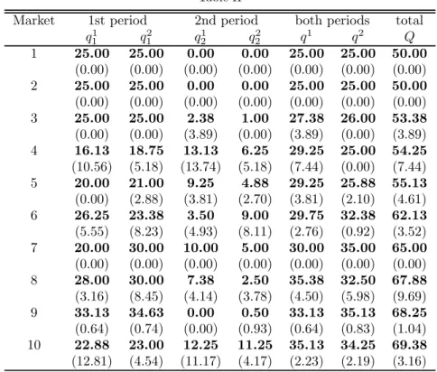
To have a better picture of behavior let us now consider disaggregate data for each of the 10 markets. Table II—taken from Müller (2006)—displays average individual quantities as observed in rounds 17 to 24 in each individual market (ordered according to increasing total output).
Table II
Market 1st period 2nd period both periods total
q1
1 q12 q12 q22 q1 q2 Q
1 25.00 25.00 0.00 0.00 25.00 25.00 50.00 (0.00) (0.00) (0.00) (0.00) (0.00) (0.00) (0.00) 2 25.00 25.00 0.00 0.00 25.00 25.00 50.00 (0.00) (0.00) (0.00) (0.00) (0.00) (0.00) (0.00) 3 25.00 25.00 2.38 1.00 27.38 26.00 53.38 (0.00) (0.00) (3.89) (0.00) (3.89) (0.00) (3.89) 4 16.13 18.75 13.13 6.25 29.25 25.00 54.25 (10.56) (5.18) (13.74) (5.18) (7.44) (0.00) (7.44) 5 20.00 21.00 9.25 4.88 29.25 25.88 55.13 (0.00) (2.88) (3.81) (2.70) (3.81) (2.10) (4.61) 6 26.25 23.38 3.50 9.00 29.75 32.38 62.13 (5.55) (8.23) (4.93) (8.11) (2.76) (0.92) (3.52) 7 20.00 30.00 10.00 5.00 30.00 35.00 65.00 (0.00) (0.00) (0.00) (0.00) (0.00) (0.00) (0.00) 8 28.00 30.00 7.38 2.50 35.38 32.50 67.88 (3.16) (8.45) (4.14) (3.78) (4.50) (5.98) (9.69) 9 33.13 34.63 0.00 0.50 33.13 35.13 68.25 (0.64) (0.74) (0.00) (0.93) (0.64) (0.83) (1.04) 10 22.88 23.00 12.25 11.25 35.13 34.25 69.38 (12.81) (4.54) (11.17) (4.17) (2.23) (2.19) (3.16) Average quantities in each market in rounds 17-24
Standard deviations in parentheses
Inspection of the last three columns in Table II reveals that, on average, roughly equal market shares are obtained and that there are almost no outcomes that resemble Stackelberg market shares. We also see that markets 1 to 5 display collusive behavior and markets 6 to 10 display Cournot-Nash behavior in the last third of the experiment.
Columns 2 and 3 in Table II show that the average (across 8 rounds)first period quantities produced in the 10 markets are smaller than or equal to the Stackelberg follower’s quantity in 14 out of 20 cases, are between the Stack-elberg follower’s quantity and the Cournot-Nash quantity in 5 out of 20 cases, and are greater than the Cournot-Nash quantity (but not significantly) in only 1 out of 20 cases. Thus, in most cases subjects produce up to the Stackelberg fol-lower’s quantity (which is equal to the collusive quantity) in thefirst production period.11
Columns 4 and 5 in Table II show thatfirms do not produce an incremental amount in the second period so that total production is equal to the Cournot-Nash quantities. Also, subjects seem to attempt to balance market shares in the second production period. Subjects who produced more in thefirst production period produce less in the second production period than subjects who produced more in the first production period. We also see that overproduction, that is, producing outside the outer envelope of the reaction functions, is rarely observed.
Huck et al. (2002) test experimentally the predictions of Hamilton and Slutsky (1990)’s action commitment game. In the experiment they use the linear inverse demand function
P(q1+q2) = max©30−(q1+q2),0ª,
and they assume that costs of production are linear and given by Ci(qi) =
6qi, i = 1,2. According to this speci
fication, the predictions of Hamilton and Slutsky (1990) are as follows. The Stackelberg leader produces in period one the quantityS = 12 and the Stackelberg follower produces in period two the quantityR(S) = 6.The simultaneous-move Cournot-Nash quantities are played in period one and are given by ¡N1, N2¢= (8,8). The collusive quantities are
(C1, C2) = (6,6). Huck et al. (2002) run an experiment with a large payoff
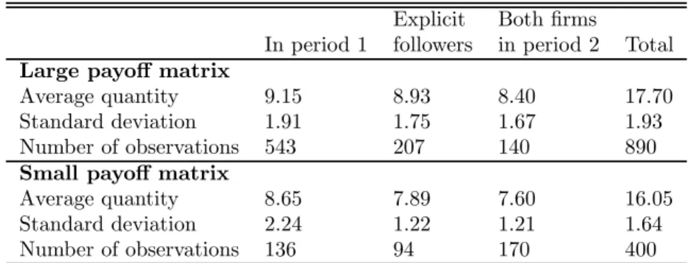
matrix where subjects could pick an integer quantity from 3 to 15 units. They also run an experiment with a small payoffmatrix where subjects could select a quantity from the set {6,8,12}. Table III—taken from Huck et al. (2002)— displays the experimental results on an aggregate level for both the large and the small payoffmatrices.
Table III
Explicit Bothfirms
In period 1 followers in period 2 Total Large payoff matrix
Average quantity 9.15 8.93 8.40 17.70
Standard deviation 1.91 1.75 1.67 1.93
Number of observations 543 207 140 890
Small payoff matrix
Average quantity 8.65 7.89 7.60 16.05
Standard deviation 2.24 1.22 1.21 1.64
Number of observations 136 94 170 400
Table III shows us that, in the experiment with the large payoff matrix, in 543 out of 890 cases (61%) subjects committed themselves in period 1. In the remaining cases subjects decided to wait. Those who decided to produce in the first period produce on average 9.15 units, which is less than the Stackelberg leader’s quantity of 12 units. Those who decided to wait and produce in the
second period after having observed that the opponent produced in the first period produce an average output of 8.93 units which is larger than the Stackel-berg follower’s output of 6 units. This seems to imply that StackelStackel-berg followers exhibit aversion to disadvantageous inequity since they are willing to produce more than the material best response to reduce the payoff of the Stackelberg leader. When both subjects decided to wait, 140 out of 890 cases (18%), their average output is 8.40 units, which is similar to the Cournot-Nash quantity. Table III also shows us that, in the experiment with the small payoffmatrix, only in 136 out of 400 cases (34%) did subjects commit themselves in thefirst period. Both subjects decided to wait in 170 out of 400 cases (42%). Average outputs are slightly smaller than those observed with the large payoffmatrix.
Huck et al. (2002) alsofind that explicit followers observed responses in the experiment with the large payoffmatrix have a curious pattern. The continuous theoretical best reply function is given by qF = 12
−0.5qL. On average, the
observed responses of followers have a negative slope when the leaders produce less than 7 units or more than 12 units. However, when leaders produces between 7 and 12 units the responses of followers have a positive slope.12 Table IV summarizes market outcomes in terms of absolute and relative frequencies for the experiment with the large payoffmatrix.
Table IV
Number Number of cases
Market outcome Type of cases incl. quant. 9 and 11
Cournot Equilibrium 64 14.4% 93 20.9%
Stackelberg Equilibrium 24 5.4% 33 7.4%
Stackelberg/Cournot Coord. failure 27 6.1% 41 9.2% Stackelberg warfare Coord. failure 21 4.7% 30 6.7%
Stackelberg punished Other 43 9.7% 55 12.4%
Collusion (successful) Other 25 5.6% 25 5.6%
Collusion (exploited) Other 19 4.3% 19 4.3%
Collusion (failed) Coord. failure 34 7.6% 41 9.2%
Others 188 42.2% 108 24.3%
Sum 445 100% 445 100%
We see from Table IV that the Cournot equilibrium is the most frequent outcome since it represents 14.4% of all outcomes—20.9% of all outcomes when the quantity 9 is counted as a Cournot action. The Stackelberg equilibria oc-cur only rarely since they represent 5.4% of all outcomes—7.4% of all outcomes when the quantity 11 is counted as a Stackelberg leader action. Coordination failure occurs in 10.8% of all outcomes—15.9% when 9 is counted as Cournot and 11 as Stackelberg leader actions. In the experiment with the small pay-off matrix Cournot outcomes become much more frequent (45% vs. 20.9%). 1 2See Fig. 2 in Huck et al. (2002). Thisfinding is replicated in Huck et al. (2001) in a
The frequencies of successful and unsuccessful collusion are similar than the ones with the large payoffmatrix. Coordination failure becomes less important (4.5% vs. 15.9%). Endogenous Stackelberg equilibria occur even less frequently (5% vs. 7.4%) than with the large matrix. The results with the small payoff
matrix rule out the possibility that complexity was responsible for the results obtained with the large payoff matrix. Thus, the results with the small payoff matrix reinforce the idea that subjects prefer symmetric Cournot outcomes to asymmetric outcomes.
Fonseca et al. (2005a) show that Huck et al. (2002)’sfindings are robust to cost asymmetries.13 Theyfind that low costfirms are not able to use their cost advantage to become Stackelberg leaders and that Cournot play is modal.14 Fonseca et al. (2005b) test experimentally Hamilton and Slutsky (1990)’ s observable delay game. In this game twofirms bindingly announce a production period (one out of two periods) and then produce in the announced sequence. Hamilton and Slutsky show that this game has a unique symmetric equilibrium where firms produce only in thefirst period. Fonseca et al. (2005b) find that there is delay in players’ production decisions.
3
The Model
Following Saloner (1987), consider a symmetric duopoly with two production periods, where the market clears at the end of the second period. In thefirst production period, firms 1 and 2 simultaneously produce outputs q1
1 and q21,
respectively. These outputs become common knowledge and, in the second production period, the firms simultaneously produce nonnegative outputs q1 2
and q2
2. After the second period, price is determined according to the inverse
demand functionP(q11+q12+q21+q22). Thefirms choose outputs to maximize expected profits. Thefirms have the same constant marginal cost of production each period,c >0.
Forfirmi, define the single-period reaction function15
Ri(qj) = arg qimax
£
P¡qi+qj¢
−c¤qi, i6=j= 1,2.
We assume that these reaction functions are well behaved.16 Let ¡N1, N2¢
be the unique single-period Cournot-Nash equilibrium outcome. When firm i
producesqiin the
first period andfirmjproduces its best response in the second 1 3We are not aware of any experiment with Saloner’s game that allows for cost asymmetries. 1 4Van Damme and Hurkens (1999, 2004) analyze a timing game with cost differences
be-tween firms. In their models a unique Stackelberg equilibrium is selected with the most efficientfirm being the Stackelberg leader.
1 5The reaction function corrresponding to a standard single production period Cournot
model.
1 6By this we mean, −1 ≤ ∂Ri(qj)/∂qi < 0.The second condition ensures the existence
of a unique single-period Cournot-Nash equilibrium. A set of sufficient conditions for Ri
functions to be “well-behaved” is thatP(qi+qj)is strictly positive on some bounded interval
period the profit function offirm iis given by
πiL=
£
P¡qi+Rj(qi)¢−c¤qi, i6=j= 1,2.
For simplicity, we assume that only one Stackelberg point exists for eachfirm. Denote these points bySi, i= 1,2,with
Si= arg qimax
£
P¡qi+Rj(qi)¢
−c¤qi, i6=j = 1,2.
Denote the outer envelope of the firms’ reaction functions, R1 and R2, by R,
and define the set
ES=
©¡
q1, q2¢:¡q1, q2¢∈R, q1≤S1, andq2≤S2ª.
Saloner (1987) shows that the following strategies for each firm constitute a subgame perfect Nash equilibrium:
q1i =ai, where ¡a1, a2¢ is a point inES
and
qi2=
⎧ ⎪ ⎪ ⎨ ⎪ ⎪ ⎩
Ni−qi
1 if qi1≤Ni andqj1≤Nj
0 if qi
1≥Ni andq j
1≤Rj(qi1)
0 if qi
1≥Ri(q1j)andq j
1≥Rj(qi1)
Ri(qj
1)−qi1 if qi1≤Ni, Nj ≤q j
1, andqi1≤Ri(q j 1)
(1)
This result says that any pair of total outputs ¡q1
1+q12, q12+q22 ¢
which lies in the outer envelope of the reaction functions between (and including) thefirms’ Stackelberg outputs is attainable with a SPNE. Furthermore, it also tells us that all production takes place in the first production period. The intuition behind this result is as follows. Let¡a¯1,¯a2¢ be a point inE
S. Without loss of
generality, let¡¯a1,¯a2¢be on R2(q1). That is, at ¡¯a1,¯a2¢ firm 1’s total output
is more than it’s single-period Cournot output andfirm 2’s total output equal it’s single-period best response toa¯1.According to the above result ¡¯a1,a¯2¢is
a SPNE and the timing of production is©¡q1
1= ¯a1, q21= 0 ¢
;¡q2
1 = ¯a2, q22= 0 ¢ª
.
The point ¡¯a1,¯a2¢ is not an equilibrium of the single-period Cournot game
since whenfirm 2 produces¯a2,firm 1 would do better to produce less than ¯a1.
However, in Saloner’s game,firm 1 cannot gain by producing less than¯a1in the
first production period, say by choosing q1
1 <¯a1. If it does, thenfirm 2 would
produce an additional amount in the second period,q2
2=R2(q11)−¯a2>0,and
this would lowerfirm 1’s profits below what it gets at ¡¯a1,¯a2¢.
firm 2 would choose the Stackelberg leadership quantity. Elimination of weakly dominated strategies also implies that in the Stackelberg equilibria the leader produces only in thefirst production period and the follower may produce only in the second period.
In Hamilton and Slutsky’s (1990) action commitment gamefirms can only produce in one of two production periods. In thefirst period firms can either produce some quantity or decide to wait. If, and only if, a firm decides to wait it is informed about the opponent’sfirst period action and after that can choose it’s second-period production. Hamilton and Slutsky show that this game has three subgame perfect Nash equilibria. One simultaneous-move Cournot equilibrium where bothfirms produce the Cournot-Nash quantities in thefirst production period.17 Two sequential-move Stackelberg equilibria where onefirm produces the Stackelberg leader’s quantity in thefirst production period and the otherfirm produces the Stackelberg follower’s quantity in the second production period.18 Thus, the set of equilibria in Hamilton and Slutsky’s game is given by
EHS=
©¡
q1 1, q21
¢
= (N, N)ª∪©¡q1 1, q22
¢
= (S, R(S))ª∪©¡q1 2, q12
¢
= (R(S), S)ª.
The Stackelberg equilibria are in undominated strategies. The simultaneous-move equilibrium uses weakly dominated strategies since playing the Cournot-Nash quantity in the first production period is dominated by waiting to play after one’s rival.
4
Inequity Aversion
Many experiments indicate that individuals are not only motivated by material self-interest, but also care about the well-being of others. We incorporate this possibility in Saloner’s game by assuming thatfirms are averse to inequality in profits. To model this, we make use of Fehr and Schmidt’s (1999) approach. Thus, we assume thatfirmi’s payoffis given by
Ui(πi,πj) =πi
−£αimax¡πj
−πi,0¢+β imax
¡
πi
−πj,0¢¤, i6=j= 1,2.
The terms in the square bracket are the payoffeffects of disadvantageous and advantageous inequity, respectively. Whenπj >πi firm i feels envy of firm j,
this is the disadvantageous inequity term. Whenπj<πifirmifeels compassion
forfirmj,this is the advantageous inequity term. Fehr and Schmidt assume that
αi andβi are nonnegative, that αi >βi,that is, the dislike of disadvantageous
1 7Both firms producing the Cournot-Nash quantities in the second production period is
not an equilibrium since eachfirm would do better by unilaterally deviate and produce the Stackelberg leader’s quantity in thefirst production period.
1 8Afirm producing the Stackelberg leader’s quantity,Si,in thefirst production period and
the opponent producing the Stackelberg follower’s quantity,Rj(Si),in the first production
inequity is stronger than that of advantageous inequity, and thatβi is smaller
than 1. We assume thatαi is nonnegative and thatβi∈[0,1/2].19
Santos-Pinto (2006) shows that the single-period reaction function offirmi, i6=j= 1,2,in the presence of inequity aversion is defined by
Ri(qj) =
⎧ ⎨ ⎩
si(qj), 0≤qj ≤q(β i)
qj, q(β
i)≤qj ≤q(αi)
ti(qj), q(αi)≤qj
,
where
si(qj) = arg
qimax (1−β i)
£
P¡qi+qj¢
−ci
¤
qi+β i
£
P¡qi+qj¢
−cj
¤
qj, (2)
ti(qj) = arg
qimax (1 +αi)
£
P¡qi+qj¢
−ci
¤
qi
−αi£P¡qi+qj¢
−cj
¤
qj, (3)
q(βi)is the solution to
(1−βi) [P(2q)−ci] +P0(2q)q= 0, (4)
andq(αi)is the solution to
(1 +αi) [P(2q)−ci] +P0(2q)q= 0. (5)
The main difference between these reaction function and the standard reaction functions is that with inequity aversion there is a range of an opponent’s output levels for which the best response of afirm is to produce the same quantity as the opponent. That happens around the Cournot-Nash equilibrium quantity of the standard simultaneous-move game. In other words, the best response has a positive slope for output levels of the opponent close to the Cournot-Nash level and a negative slope for the remaining output levels of the opponent. As we have seen, Huck et al.’s (2002) experiment on Hamilton and Slutsky’s action commitment gamefind evidence for this type of reaction function.
Santos-Pinto (2006) also shows that the set of Nash equilibria of the single-period symmetric Cournot duopoly game whenfirms are averse to inequity is given by
EIA=©¡q1, q2¢:q1=q2, andN(β1,β2)≤qi≤N(α1,α2), i= 1,2ª,
whereN(β1,β2) = max [q(β1), q(β2)],andN(α1,α2) = min [q(α1), q(α2)].
This result tells us that inequity aversion betweenfirms gives rise to a con-tinuum of symmetric equilibria in the single-period Cournot duopoly game. The intuition for this result is as follows. Suppose that afirm knows it’s opponent will produce an output level that is close to the Nash equilibrium of the stan-dard single-period Cournot game. If thatfirm dislikes inequity aversion, then
1 9The assumption thatβ
iis smaller than1/2implies that afirm never cares more about the
there is a cost in advantageous inequity associated with producing a higher level of output than the opponent. Similarly, there is also a cost in disadvantageous inequity associated with producing a smaller output level than the opponent. For a range of output levels close to the Nash equilibrium of the standard single-period Cournot game the profits lost from not matching the opponent’s output are small while the inequity costs are large. If that is the case then thefirm is better offby producing the same level of output as the opponent.
The result also shows that the smallest Nash equilibria of the single-period Cournot game is determined by the lowest level of compassion of the twofirms and that the largest Nash equilibria is determined by the lowest level of envy of the twofirms. We see from (2) that if bothfirms have a level of compassion equal to 1/2, then the lowest Nash equilibrium of the single-period Cournot duopoly game with inequity aversefirms corresponds to the collusive outcome. We will now show that inequity aversion between firms also gives rise to a continuum of symmetric equilibria in Saloner’s two-period Cournot duopoly game. We start our analysis by stating a lemma that characterizes a firm’s second-period equilibrium output in Saloner’s game with inequity aversefirms. Saloner (1987) proved this lemma in the standard two-period Cournot duopoly game with selfish firms. To prove our lemma we assume, without loss of gen-erality, that there is symmetry in the inequity aversion parameters, that is, we take α1 = α2 = α and β1 = β2 = β.20 Given this assumption, we let N(β)
denote N(β1,β2)and N(α) denote N(α1,α2). We are now ready to state the
lemma.
Lemma 1 Given thefirst-period outputs (q1
1, q21), the second-period equilibrium
outputs forfirm i,i= 1,2,are as follows:
qi 2= ⎧ ⎪ ⎪ ⎪ ⎪ ⎪ ⎪ ⎪ ⎨ ⎪ ⎪ ⎪ ⎪ ⎪ ⎪ ⎪ ⎩
0 if qi
1≥ti(qj1), andq j
1≥tj(qi1)
N(β)−qi
1 if q1i ≤N(β), andq j
1≤N(β)
qj1−qi
1 if q1i ≤q1j, andN(β)≤q j
1≤N(α)
0 if N(β)≤qi
1≤N(α), andq j 1≤qi1
0 if qi
1≥N(α), andq1j≤tj(q1i)
ti(qj
1)−q1i if q1i ≤N(α), N(α)≤q j
1, andq1i ≤ti(q j 1)
, (6)
where ti is given by (3).
This lemma says if ¡q1 1, q12
¢
lies on or outside the outer-envelope of t1(q2)
and t2(q1), then neither firm produces in the second period. If ¡q1 1, q12
¢
lies inside the outer-envelope oft1(q2)and t2(q1), then there are three cases to be
considered. If bothfirms have produced less thanN(β)in thefirst period,then each produces up toN(β)in the second period. Iffirmjhas producedq1j,where
q1j is more thanN(β)but less thanN(α),andfirmihas produced less thanq1j,
thenfirm i produces it’s best response tofirm j’s first period output and firm
j does not produce at all. In this case, both firms end up producing the same 2 0If we assume that β
1 6=β2 and/orα1 6=α2 the game becomes asymmetric andfirms’
amount since inequity aversion implies that firm i’s best response tofirm j’s first period output is to produce as much as firm j. If one firm has exceeded
N(α)but the other has not, then the latter produces it’s best response to the former’s first period output and the former does not produce at all. In this case, the firm that has exceeded N(α) produces more than the firm that has not exceededN(α).
By comparing (1) to (6) we can see that inequity aversion between firms changes the second-period equilibrium outputs in two ways. First, there is a range of first-period output levels for which the best response of a firm is to produce the same level of output as the opponent. This happens because producing the same level of output as the opponent implies afirst order gain in reduction of inequity costs and a second order loss in material payoff. Second, there is another range offirst period outputs for which the best response of a firm is shifted by comparison with the best response in the absence of inequity aversion. This happens because, for this other range offirst period output levels, thefirm that produces the smallest output level in thefirst production end ups feeling envy towards the opponent. This implies that the second-period output of thefirm that feels envy is larger than the output it would have produced in the second period if it felt no envy.
We will use lemma 1 to characterize the set of equilibria of Saloner’s game with inequity aversefirms. Before doing that we need to introduce some nota-tion. Let the Stackelberg leader’s quantity in the presence of inequity aversion be denoted by Si(α,β), i = 1,2 and the Stackelberg follower’s quantity by
Rj(Si(α,β)), j 6=i. If firm i is the Stackelberg leader, then it picks the point
inRj(qi)that maximizes its payoff. The existence of inequity aversion implies
that the Stackelberg leader’s quantity is defined as
Si(α,β) =
½
N(β), if Ui(Li(α,β), tj(Li(α,β)))≤Ui(N(β), N(β))
Li(α,β), otherwise ,
(7) and the Stackelberg follower’s quantity by
Rj¡Si(α,β)¢=
½
N(β), if Ui(Li(α,β), tj(Li(α,β)))≤Ui(N(β), N(β))
tj¡Li(α,β)¢, otherwise ,
(8) where
Li(α,β) = argqi
≥N(α)max (1−β) £
P¡qi+tj(qi¢)−ci
¤
qi +β£P¡qi+tj(qi¢)
−cj
¤
tj(qi),
j6=i= 1,2.We see from (7) and (8) that the presence of inequity aversion im-plies that the Stackelberg point is either point(N(β), N(β)),the smallest Nash equilibrium of the simultaneous-move game, or point ¡Li(α,β), tj¡Li(α,β)¢¢.
is the Stackelberg point. If the payoffof the smallest Nash equilibrium of the si-multaneous move game is smaller than the payoffof point¡Li(α,β), tj¡Li(α,β)¢¢,
then point¡Li(α,β), tj¡Li(α,β)¢¢ is the Stackelberg point. In this case, firm
i produces more than firm j since Li(α,β) < tj¡Li(α,β)¢. This implies that
the material payoff of firm i is larger than the material payoff of firm j and thereforefirm i feels compassion towards firm j whereasfirm j feels envy to-wardsfirmi. We also see from (7) and (8) that if the Stackelberg point is point
¡
Li(α,β), tj¡Li(α,β)¢¢,then it a function of αand ofβ. An increase in envy
reduces Li(α,β) and so does an increase in compassion. If the degree of envy
increases, this leads the follower to raise production and this in turn implies a lower quantity for the leader. Also, if the degree of compassion of the leader increases, then the leader reduces its output to reduce inequity aversion.
Proposition 1 characterizes the set of equilibria of Saloner’s game for rela-tively high levels of inequity aversion betweenfirms.
Proposition 1 If Ui(N(β), N(β))> Ui(Si(α,β), tj(Si(α,β))),i= 1,2, then the set of equilibria of Saloner’s game with inequity aversefirms is given by
EIA S =
©¡
q1, q2¢:q1=q2,and N(β)≤qi
≤N(α), i= 1,2ª.
This result tells us that if the degree of inequity aversion between firms is relatively high, then Saloner’s game has a continuum of symmetric SPNE. The set of equilibria is any pair of total outputs wherefirms produce the same quantity, that isq1
1+q21=q12+q22,and where the quantities produced by the two
firms are between the smallest and the largest Nash equilibrium of the single-period Cournot duopoly game with inequity averse firms. Thus, if the degree of inequity aversion between firms is relatively high, then the set of SPNE of Saloner’s game coincides with the set of Nash equilibria of the single-period Cournot duopoly game.
The intuition for this result is straightforward. Inequity aversion between firms, no matter if it is high or low, gives rise to a continuum of symmetric equilibria both in the single-period Cournot game as well as in Saloner’s duopoly game. Inequity aversion between firms makes symmetric outcomes in the set
EIA
S more desirable tofirms than unilateral deviations to asymmetric outcomes.
This happens because any unilateral deviation away from a symmetric outcome inEIA
S with N ≤ qi ≤N(α), i = 1,2, leads to an inequity cost and a loss in
material payoffand any unilateral deviation from a symmetric outcome inEIA S
withN(β)≤qi ≤N, i= 1,2,leads to afirst order inequity cost and a second
order gain in material payoff.
Relatively high levels of inequity aversion rule out asymmetric equilibria. If
choosing afirst period production that leads to asymmetric quantities and so the game has no asymmetric equilibria.21
Our next result characterizes the set of equilibria of Saloner’s game for rel-atively low levels of inequity aversion betweenfirms.
Proposition 2 If α and β are such that the Stackelberg point exists and
Ui(Si(α,β), Rj(Si(α,β)))> Ui(N(β), N(β)),i= 1,2,then the set of equilibria of Saloner’s game with inequity aversefirms is given by
EIA S =
©¡
q1, q2¢:q1=q2,and N(β)≤qi
≤N(α), i= 1,2ª
∪n¡q1, q2¢:t2(L1(α,β))≤q2≤q(ˆα,β), q1=¡t2¢−1(q2)o
∪n¡q1, q2¢:t1(L2(α,β))≤q1≤q(ˆα,β), q2=¡t2¢−1(q1)o,
where q(ˆα,β)is the solution toUi(N(β), N(β)) =Ui(qi, tj(qi)).
This result tells us that if the degree of inequity aversion betweenfirms is rel-atively low, then Saloner’s game has a continuum of symmetric and asymmetric SPNE. Like in Proposition 1, the set of equilibria is any pair of total outputs where firms produce the same quantity and where the quantities produced by the twofirms are between the smallest and the largest Nash equilibrium of si-multaneous move game. Additionally, the set of equilibria is also composed of any point on the outer envelope of the reaction function offirm ibetweenfirm
i’s Stackelberg leader’s output and output levelq(ˆα,β), i= 1,2.
This result is not surprising. If the level of inequity aversion is relatively low, then unilateral deviations from asymmetric outcomes to symmetric outcomes may no longer be desirable. This happens because as inequity aversion decreases the gains in inequity costs from playing symmetric outcomes become smaller than the losses in material payoffs. If that is the case there must be sufficiently low levels of inequity aversion for which Saloner’s game has asymmetric equilib-ria. Proposition 2 states the conditions for this to happen and characterizes the set of asymmetric equilibria. It tells us that ifαandβ are relatively low, then 2 1To characterize the condition that defines what we call relatively high levels of
in-equity aversion consider a linear demand: P =a−bQ.In this case we have that N(β) =
1−β
3−2β
a−c
b and S
i(α,β) = (1−2β)(1+α)2
(1+2α)(2+2α−3β−2αβ) a−c
b . The condition U
i(N(β), N(β))
≥
Ui(Si(α,β), tj(Si(α,β)))becomes
(1−β) (3−2β)2
(a−c)2
b ≥
(1 +α−β)2
4 (1 + 2α) (2 + 2α−3β−2αβ) (a−c)2
b , or
4 (1−β) (1 + 2α) (2 + 2α−3β−2βα)≥(3−2β)2(1 +α−β)2. Solving the condition as an equality with respect toαwe have
α= 1 2 (6β−7)
µ
−4β2−2β+ 6−4q¡4β4−16β3+ 25β2−17β+ 4¢
¶
.
the Stackelberg point is given by¡Li(α,β), tj¡Li(α,β)¢¢.This point is an
equi-librium of the two-period game since the conditionUi(Si(α,β), tj(Si(α,β)))≥
Ui(N(β), N(β)) implies that the Stackelberg leader does not wish to deviate
from the Stackelberg quantity to N(β), the best symmetric equilibrium quan-tity. It also follows that there is a set of points ontj(·)such thatq(ˆα,β)< qi <
Li(α,β) which are also asymmetric equilibria since the payoff at these points
is larger than the payoffof the smallest Nash equilibrium of the simultaneous move game.
Santos-Pinto (2006) shows that the point(N(β), N(β))is decreasing withβ,
that is, the smallest symmetric equilibrium of the single-period Cournot duopoly game with inequity aversefirms is decreasing with an increase in compassion. This means, that an decrease in compassion moves the set of symmetric equi-librium outcomes closer to the collusive outcome (the outcome obtained when
β= 1/2). By contrast, the largest symmetric equilibrium of the single-period Cournot duopoly game with inequity aversefirms is increasing with an increase in envy.
Obviously, these results also apply to the set of symmetric equilibria of Saloner’s game with inequity aversefirms. As α and β converge to zero the impact of inequity aversion vanishes. As the impact of inequity aversion vanishes the set of symmetric equilibria in Saloner’s game with inequity aversion collapses to the Nash equilibria of the single-period Cournot game.22 By contrast, as the impact of inequity aversion vanishes the set of asymmetric equilibria in Saloner’s game with inequity aversion expands.23
Let us now consider the impact of inequity aversion on the set of equilibria in Hamilton and Slutsky’s action commitment game. The next result characterizes the set of equilibria of this game for relatively high levels of inequity aversion. Proposition 3 If Ui(N(β), N(β))> Ui(Si(α,β), tj(Si(α,β))), i= 1,2,then the set of equilibria of Hamilton and Slutsky’s action commitment game with inequity aversefirms is given by
EIA HS=
©¡
q11, q21¢:q11=q21,and N(β)≤qi
1≤N(α), i= 1,2 ª
∪©¡q21, q22¢= (N(β), N(β))ª.
This result tells us that if the degree of inequity aversion between firms is relatively high, then Hamilton and Slutsky’s action commitment game has a continuum of symmetric SPNE. The set of equilibria is any pair of outputs wherefirms produce the same quantity, they do it in thefirst production period, and where the quantities produced by the twofirms are between the smallest and the largest Nash equilibrium of the single-period Cournot duopoly game with inequity averse firms. Thus, if the degree of inequity aversion between firms is relatively high, then the set of SPNE of Hamilton and Slutsky’s action 2 2Asαconverges to zero the point(N(α), N(α))converges to(N, N)and asβconverges to
zero the point(N(β), N(β))converges to(N, N).
2 3Asαandβconverge to zero the point¡Si(α,β), tj(Si(α,β))¢converges to¡Si;Rj(Si)¢,
commitment game coincides with the set of Nash equilibria of the single-period Cournot duopoly game.24
The intuition for this result is as follows. Inequity aversion betweenfirms, no matter if it is high or low, gives rise to a continuum of symmetric equilibria both in the single-period Cournot game as well as in Hamilton and Slutsky’s game. Additionally, if inequity aversion is relatively high, that is,αandβare such that eachfirm prefers the smallest Nash equilibrium payoffof the simultaneous move game, Ui(N(β), N(β)) to its payoff as the Stackelberg leader, then there are
no Stackelberg equilibria. Thus, the only equilibria of Hamilton and Slutsky’s action commitment game with relatively high levels of inequity aversion between firms are the simultaneous-move equilibria. The fact that in Hamilton and Slutsky’s action commitment game firms can only produce in one of the two periods implies that production in any simultaneous move-equilibria takes place in thefirst period.
The fact that there exists a continuum of symmetric equilibria and that firms must coordinate by moving simultaneously in the first production period is consistent with the empiricalfinding that there is more coordination failure in Hamilton and Slutsky’s action commitment game than in Saloner’s game.
The next result characterizes the set of equilibria in Hamilton and Slutsky’s action commitment game for relatively low levels of inequity aversion.
Proposition 4 If α and β are such that the Stackelberg point exists and
Ui(Si(α,β), Rj(Si(α,β)))> Ui(N(β), N(β)),i= 1,2,then the set of equilibria of Hamilton and Slutsky’s action commitment game with inequity aversefirms is given by
EHSIA =
©¡
q11, q21¢:q11=q21,and N(β)≤qi1≤N(α), i= 1,2ª
∪©¡q11, q22¢= (L1(α,β), t2(L1(α,β)))ª∪©¡q21, q21¢= (t1(L2(α,β)), L2(α,β))ª.
This result tells us that if the degree of inequity aversion between firms is relatively low, then Hamilton and Slutsky’s action commitment game has a continuum of symmetric SPNE and two asymmetric SPNE. In any symmet-ric equilibria both firms produce in the first period and eachfirm produces a quantity between the smallest and the largest Nash equilibrium quantity of the single-period Cournot duopoly game with inequity averse firms. The asym-metric equilibria are of the leader follower type with one firm producing the Stackelberg leader’s quantity in thefirst production period and the other firm producing the Stackelberg follower’s quantity in the second period. The dif-ference here, by comparison with Hamilton and Slutsky’s action commitment game with selfish firms, is that a compassionate leader produces less than a selfish leader and a envious follower produces more than a selfish follower.
2 4This is true for any symmetric equilibria inEIA
HS,except the lowest Nash equilibrium of
the simultanous-move Cournot game,(N(β), N(β)). Suppose that bothfirms produceN(β)
in the second production period. In this case ,eachfirm is indifferent between producingN(β)
5
Summary and Comparison
In this section we summarize the predictions of the inequity aversion explanation for Saloner’s game and for Hamilton and Slutsky’s action commitment game. We also compare the predictions to the experimental evidence. Table V below summarizes the predictions for Saloner’s game.
Table V
Saloner’s Duopoly Game
Sym. Asym Coll. Stack. Time Balance Prod.
eq. eq. out. warf. prod. shares P1
Ineq. Av.
High Many - Yes Yes P1&P2 Yes No
Low Many - No No P1&P2 Yes No
- Many - - P1&P2 - No
Recall that the experimental evidence on Saloner’s game tells us that: (i) Stackelberg outcomes are extremely rare, (ii) simultaneous-move symmetric out-comes are the most frequent outout-comes, (iii) sometimes collusive outout-comes are observed, (iv) there is production in both periods with 84% of production taking place in thefirst period, (v) subjects seem to attempt to balance market shares in the second production period, and (vi) subjects do not produce more than the Stackelberg follower’s quantity in thefirst production period.
Table V shows us that the predictions of the inequity aversion explanation are consistent with most of the experimental evidence on Saloner’s game. First, relatively high levels of inequity aversion imply that Saloner’s game has a con-tinuum of simultaneous-move symmetric equilibria. Among all the symmetric equilibria the Cournot-Nash equilibrium may be the one that is more frequently played because it is always a subgame perfect Nash equilibrium of the game no matter if there is inequity aversion or not. This is no longer true for other symmetric equilibria. When inequity aversion is low there is still a continuum of simultaneous-move symmetric equilibria but there is also a continuum of asymmetric equilibria where play may be sequential.
Second, inequity aversion is also able to explain the fact that in some games “collusive outcomes” are played. This can happen whenever two subjects with a high degree of compassion are matched to play the game and are able to coordinate on the collusive outcome. Similarly, inequity aversion is also able to explain the fact that in some games there is Stackelberg warfare. This can happen whenever two subjects with a high degree of envy are matched to play the game and both produce more than the Cournot-Nash quantities.
Third, relatively high levels of inequity aversion rule out Stackelberg out-comes. However, relatively low levels of inequity aversion do not. Thus, when-ever two subjects with a relatively low level of inequity aversion are matched to play the game we may have Stackelberg equilibria.
gives rise to a multiplicity of symmetric equilibria in the game and subjects have to coordinate on one of them. If subjects are unable to coordinate in one of the multiple symmetric equilibria in thefirst production period, then they have an incentive to produce in the second production period to attain coordination before the market clears.
Fifth, inequity aversion also predicts that subjects attempt to balance mar-ket shares. This happens whenever subjects fail to coordinate on a symmetric equilibrium in thefirst production period. In those cases, the subject who pro-duced less in thefirst production period will produce a positive amount in the second period whereas the subject who produced more in the first production period will not produce in the second production period.
The only empiricalfinding in Saloner’s game that the inequity aversion ex-planation seems unable to account for is the fact thatfirms do not produce more than the Stackelberg follower’s quantity in thefirst production period.
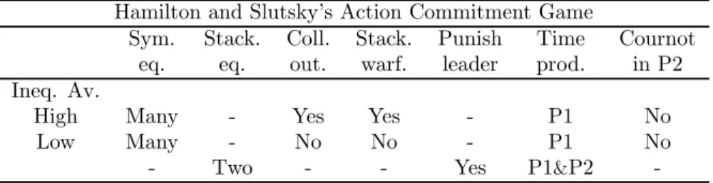
Table VI below summarizes the predictions for Hamilton and Slutsky’s action commitment game.
Table VI
Hamilton and Slutsky’s Action Commitment Game
Sym. Stack. Coll. Stack. Punish Time Cournot
eq. eq. out. warf. leader prod. in P2
Ineq. Av.
High Many - Yes Yes - P1 No
Low Many - No No - P1 No
- Two - - Yes P1&P2
-Recall that the experimental evidence on Hamilton and Slutsky’s action com-mitment game tells us that: (i) Stackelberg outcomes are rare, (ii) move Cournot outcomes are the most frequent outcomes, (iii) simultaneous-move outcomes are often played in the second production period, and (iv) be-havior is quite heterogeneous—in some cases followers punish leaders, in other cases collusive outcomes are played, and in other cases Stackelberg warfare is observed.
Table VI shows us that inequity aversion is also able to explain most of the experimental evidence on Hamilton and Slutsky’s action commitment game. First, relatively high levels of inequity aversion imply that Hamilton and Slut-sky’s action commitment game only has simultaneous-move symmetric outcomes where bothfirms produce in thefirst production period.25 When inequity aver-sion is low there is a continuum of simultaneous-move symmetric equilibria but there are also two Stackelberg equilibria with sequential play.
2 5Like in Saloner’s game with inequity aversefirms, among all the symmetric equilibria in
Second, inequity aversion can explain collusive outcomes in Hamilton and Slutsky’s action commitment game. This happens whenever both players have a relatively high level of inequity aversion and they are able to coordinate on the collusive outcome.
Third, if inequity aversion is relatively high there are no Stackelberg out-comes in Hamilton and Slutsky’s action commitment game. So, for Stackelberg outcomes to be played players must have relatively low levels of inequity aver-sion.
Fourth, if inequity aversion is relatively low and players play the Stackelberg outcome, then the model predicts that the Stackelberg leader will feel compas-sion towards the follower and that the Stackelberg follower will feel envy towards the leader. This implies that a compassionate leader produces less than a selfish leader and that an envious follower produces more than a selfish follower. This pattern is consistent with the evidence in Huck et al. (2002). Table III shows that in the experiment with the large payoffmatrix, explicit followers produce on average 8.93 units. This is significantly higher than the Stackelberg follower’s quantity of 6 units.26
The only empirical finding in Hamilton and Slutsky’s action commitment game that inequity aversion is unable to explain is simultaneous-move Cournot-Nash outcomes in the second production period.27
6
Extensions
As we have seen, Fehr and Schmidt’s (1999) model of inequity aversion is able to explain several experimentalfindings in endogenous timing games. However, Fehr and Schmidt’s specification is a particular functional form of inequity aver-sion (it is piecewise linear and non-differentiable). Could it be that the results obtained extend to more general preferences?
2 6The same happens in the experiment with the small payoffmatrix. On average, explicit
followers in the experiment with the small payoffmatrix produce 7.89. Huck et al. (2002) do not display data for explicit leaders. However, we can use the data in the small payoffmatrix to have an idea of the average quantity of explicit leaders (in the small payoffmatrix most players who produce in thefirst period are explicit leaders, this is not the case in the large payoff matrix). In the experiment with the small payoff matrix there are 136 players who produce in thefirst period, of which 94 are explicit leaders and 42 are players who produce simultaneously. If the 94 explicit leaders produced the leader’s quantity, 12 units, and the other 42 players the Cournot-Nash quantity, the average output of these 136 players should be equal to 10.76. By contrast, the data shows that the average output of these 136 players is significantly lower: 8.65 units. This tells us that, on average, explicit leaders produce substantially less than the Stackelberg quantity.
2 7Fonseca et al. (2005b) test experimentally Hamilton and Slutsky (1990)’ s observable
Santos-Pinto (2006) studies the impact of general forms of inequity aver-sion on Cournot competition. He shows that for differentiable forms of inequity aversion the best reply of a firm is always negatively sloped. However, the best reply of an inequity averse firm is smaller than the best reply of a self-ish firm when the rival produces low output levels (the inequity averse firms fells compassion for the rival) and the best reply of an inequity averse firm is larger than that of a selfish firm when the rival produces high output levels (the inequity averse firm feels envy towards the rival). This implies that the set of SPNE of Saloner’s game with differentiable inequity aversion is closer to the 45odegree line, than the set of SPNE of Saloner’s game with selfish firms.
The same happens in Hamilton and Slutsky’s (1990) endogenous timing game. The Stackelberg equilibria of Hamilton and Slutsky’s action commitment game withfirms with differentiable inequity aversion are much less asymmetric than the Stackelberg equilibria obtained with selfish firms. Thus, inequity aversion either rules out asymmetric outcomes completely (high levels of piecewise linear inequity aversion) or reduces the degree of asymmetry substantially (high levels of differentiable inequity aversion).
The fact that differentiable inequity aversion does not lead to positively sloped best replies for intermediate output levels of the rival implies that the continuum of equilibria result obtained with piecewise linear aversion is no longer valid. This in turn implies that differentiable inequity aversion can no longer explain production in both periods in Saloner’s game as well as thefinding that players try to balance market shares in the second production period.
Besides inequity aversion, reciprocity, is another common type of other-regarding preferences. A reciprocal agent cares about the intentions of his rivals. He responds to actions that he perceives to be harmful in a harmful manner and he responds to actions that he perceives to be kind in a kind manner. Santos-Pinto (2006) shows that the impact of reciprocity on Cournot competition is similar to that of inequity aversion. Thus, the results in this paper also extend to players with reciprocal preferences.
7
Conclusion
of the experimental evidence on endogenous timing games.
References
Bagwell, K (1995). “Commitment and Observability in Games,” Games and Economic Behavior, 8, 271-280.
Ellingsen, T. (1995). “On Flexibility in Oligopoly,”Economic Letters, 48, 83-89. Fehr, E. and K. Schmidt (1999). “A Theory of Fairness, Competition, and Cooperation,”Quarterly Journal of Economics, 114, 817-868.
Fonseca, M, S. Huck, and H.-T. Normann (2005a). “Playing Cournot Although they Shouldn’t: Endogenous Timing in Experimental Duopolies with Asymmet-ric Cost,”Economic Theory, 25, 669-677.
Fonseca, M, S. Huck, and H.-T. Normann (2005b). “Endogenous Timing in Duopoly: Experimental Evidence,” Discussion Paper No. 2005-77, Tilburg Uni-versity.
Hamilton, J, and S. Slutsky (1990). “Endogenous Timing in Duopoly Games: Stackelberg or Cournot Equilibria,”Games and Economic Behavior, 2, 29-46. Harsanyi, J., and R. Selten (1988). A General Theory of Equilibrium Selection in Games, Cambridge, MA: MIT Press.
Huck, S., W. Müller, and H.-T. Normann (2001). “Stackelberg Beats Cournot-On Collusion and Efficiency in Experimental Markets,”Economic Journal, Vol. 111, 749-765.
Huck, S., W. Müller, and H.-T. Normann (2002). “To Commit or Not to Com-mit: Endogenous Timing in Experimental Duopoly Markets,”Games and Eco-nomic Behavior, 38, 240-264.
Maggi, G. (1996). “Endogenous Leadership in a New Market,” Rand Journal of Economics, 27(4), 641-659.
Müller, W. (2006). “Allowing for Two Production Periods in the Cournot Duopoly: Experimental Evidence,”Journal of Economic Behavior and Organi-zation, 60(1), 100-111.
Robson, A. (1990). “Duopoly with Endogenous Strategic Timing: Stackelberg Regained,”International Economic Review, 31(2), 263-274.
Saloner, G. (1987). “Cournot Duopoly with Two Production Periods,”Journal of Economic Theory, 42, 183-187.
Santos-Pinto, L. (2006). “Reciprocity, Inequity Aversion, and Oligopolistic Competition,” Working Paper, Universidade Nova de Lisboa.