Essays on the role of contagion and integration in international issues of South America

(1)

UNIVERSIDADE FEDERAL DO CEARÁ

FACULDADE DE ECONOMIA, ADMINITRAÇÃO, ATÚARIA E ECONOMIA PROGRAMA DE PÓS-GRADUAÇÃO EM ECONOMIA - CAEN

FELIPE ALVES REIS

ESSAYS ON THE ROLE OF CONTAGION AND INTEGRATION IN INTERNATIONAL ISSUES OF SOUTH AMERICA

(2)

Tese apresentada ao Programa de Pós-Graduação em Economia - CAEN, da Faculdade de Economia, Administração, Atuária e Contabilidade da Universidade Federal do Ceará, como requisito parcial à obtenção do título de Doutor em Ciências Econômicas. Área de concentração: Finanças Internacionais Aplicadas.

Orientador: Prof. Dr. Paulo Rogério Faustino de Matos.

(3)

Dados Internacionais de Catalogação na Publicação Universidade Federal do Ceará

Biblioteca Universitária

Gerada automaticamente pelo módulo Catalog, mediante os dados fornecidos pelo(a) autor(a)

R31e Reis, Felipe Alves.

ESSAYS ON THE ROLE OF CONTAGION AND INTEGRATION IN INTERNATIONAL ISSUES OF SOUTH AMERICA / Felipe Alves Reis. – 2017.

94 f. : il. color.

Tese (doutorado) – Universidade Federal do Ceará, Faculdade de Economia, Administração, Atuária e Contabilidade, Programa de Pós-Graduação em Economia, Fortaleza, 2017. Orientação: Prof. Dr. Paulo Rogério Faustino Matos.

(4)

Tese submetida à coordenação do programa de Pós-Graduação em Economia - CAEN da Faculdade de Economia, Administração, Atú aria e Contabilidade da Universidade Federal do Ceará, como requisito parcial à obtenção do título de Doutor em Ciências Econômicas. Área de concentração: Finanças Internacionais Aplicadas.

Aprovada em: ___/___/______.

BANCA EXAMINADORA

________________________________________________ Prof. Dr. Paulo Rogério Faustino de Matos (Orientador)

Universidade Federal do Ceará (UFC)

________________________________________________ Prof. Ricardo Antônio de Castro Pereira

________________________________________________ Prof. Dr. Sérgio Aquino de Souza

________________________________________________ Prof. Dr. Nicolino Trompieri Neto

Instituto de Pesquisa e Estratégia Econômica do Ceará (IPECE)

________________________________________________ Prof. Dr. Leonardo Andrade Rocha

(5)

A Deus.

(6)

AGRADECIMENTOS

Nesse momento tão especial da minha vida, não poderia deixar de agradecer as pessoas que de alguma forma contribuíram para que eu alcançasse o meu objetivo.

Agradeço a Deus, em primeiro lugar, por ter me concedido o dom da vida, força, saúde e principalmente determinação para que eu pudesse finalizar este trabalho.

Agradeço aos meus pais, José Barbosa Reis e Maria Gerileuza Alves Reis, pelo grande amor,

apoio, compreensão e solidariedade em todos os momentos de minha vida, me ensinando sempre a caminhar, mas deixando-me tropeçar por horas para aprender a não mais cair e ainda acreditar que eu seria capaz de conseguir o que desejaria nesta grande batalha que é a vida. Obrigado! Em especial a minha esposa, Kellvia que durante os nossos quase 17 anos juntos, sempre tem me dado apoio, amor, carinho nos momentos difíceis e uma filha maravilhosa. Sem esses incentivos, com certeza, não teria conseguido. Te amo e obrigado!

Ao professor Paulo Rogério Faustino de Matos, com quem tenho aprendido bastante em que temos trabalhado juntos e cujos ensinamentos levarei para a vida toda, pelo grande apoio, compreensão e solidariedade em todos os momentos de minha vida, me ensinando sempre a caminhar, mas deixando-me tropeçar por horas para aprender a não mais cair e ainda acreditar que eu seria capaz de conseguir o que desejaria nesta grande batalha que é a vida.

Aos professores Ricardo Antônio de Castro Pereira, Sérgio Aquino de Souza, Nicolino Trompieri Neto e Leonardo Andrade Rocha por disponibilizarem seu tempo para participar da banca de avaliação e por suas contribuições ao trabalho.

Aos demais professores do CAEN por suas contribuições à minha formação académica. A todos os funcionários do CAEN.

Agradeço também a todos os colegas de Mestrado e Doutorado do CAEN. Por _ﬁm, agradeço ao CAEN por disponibilizar sua estrutura para a realização deste trabalho e a CAPES pela bolsa concedida.

(7)

RESUMO

As economias emergentes da América do Sul atraem comumente a atenção de pesquisadores, mesmo que por razões pontualmente distintas entre as economias em questão. Dentre essas economias pode-se destacar o sólido mercado financeiro chileno, a consolidada demanda interna da população brasileira, a convergência antidemocrática argentina, o processo de pacificação interna colombiana, ou mesmo as elevadas taxas de crescimento da economia

peruana. Adicionalmente a isso, ressaltamos os resultados de Matos, Siqueira & Trompieri (2014) que evidenciam a existência de um elevado nível de integração e o contágio financeiro entre os índices do Brasil, Argentina, Colômbia, Chile, Peru e Venezuela. À luz dessas evidências, essa tese faz três ensaios acerca de dados financeiros e econômicos do Brasil, Argentina, Colômbia, Chile e Peru. No primeiro ensaio faz-se a análise do mercado de risco dessas economias através da metodologia Value at Risck - VaR condicional, onde o valor crítico que caracteriza o VaR foi associado à distribuição que apresentar melhor fitting e incorporamos os efeitos da média e da volatilidade, ambas condicionais, obtidas pelo arcabouço ARMA-GARCH mais bem especificado. Onde observa-se que os modelos condicionais best fitting tem uma menor quantidade de violações. No segundo ensaio, buscou a análise das reservas internacionais seguindo conceitualmente noções da metodologia Buffer

Stock, porém considerando os efeitos cruzados significativos das volatilidades condicionais, dos respectivos spreads e das importações intrablocos. Os resultados apontam uma melhoria significativa no poder explicação do modelo e que as reservas brasileiras são a menos afetadas pelas economias da América do Sul. No último ensaio foi analisado as opções de carteiras diversificadas disponíveis para um investidor brasileiro, que enfrenta um cenário livre de oportunidades no mercado financeiro, com o objetivo de mensurar ganhos com diversificação da posição adquirida nos índices de mercado da América do Sul vis-à-vis um carteira doméstica. Os resultados mostram a possibilidade que estratégias de composição de carteira simples e não dinâmica, composta somente de índices dos mercados dos países vizinhos do

Brasil, se traduzam em resultados muito satisfatórios em termos de ganho e risco esperados.

(8)

ABSTRACT

The emerging economies of South America commonly attract the attention of researchers, even if for punctually different reasons among the economies in question. These economies include the strong Chilean financial market, the consolidated domestic demand of the Brazilian population, the Argentine anti-democratic convergence, the process of internal pacification in Colombia, or even the high growth rates of the Peruvian economy. In addition

to this, we highlight the results of Matos, Siqueira & Trompieri (2014) that show the existence of a high level of integration and the financial contagion among the indices of Brazil, Argentina, Colombia, Chile, Peru and Venezuela. In light of these evidences, this thesis presents three essays on financial and economic data from Brazil, Argentina, Colombia, Chile and Peru. In the first essay, we analyze the risk market of these economies using the Value at Risck - VaR conditional methodology, in which the critical value that characterizes the VaR is associated to the distribution that presents the best fitting, and we incorporate the effects of the mean and the volatility, both conditional, obtained by the best-specified ARMA-GARCH model, showing that the best fitting conditional models have a smaller number of violations. The second essay presents the analysis of international reserves, conceptually following the notions of the Buffer Stock methodology, but considering the significant cross-effects of conditional volatilities, their respective spreads and intra-block importation.The results point to both a significant improvement in the explanatory power of the model and that the Brazilian reserves are the least affected by South American economies. In the last essay, we analyze some diversified portfolio options available to a Brazilian investor, who faces a scenario with no opportunities in the financial market, with the purpose of measuring gains with diversification of the position acquired in the South American market indices vis-à-vis the domestic portfolio.The results show the possibility that simple and non-dynamic portfolio composition strategies, composed only of indexes of the markets of the neighboring countries of Brazil, translate into very satisfactory results in terms of expected gain and risk.

(9)

LIST OF FIGURES

Figure 2.1 - Cumulative daily return on South American stock market indices... 28

Figure 2.2 - Nominal net returns on South American major Market indices... 31

Figure 2.3 - Conditional volatility of returns on South American stock market indices………... 35

Figure 2.4 - Laplace-based absolute VaR (99%, 01 day) of South American stock market indices………... 36

Figure 3.1 - Total reserves excluding gold (U$$ million)………... 48

Figure 3.2 - Total reserves excluding gold (U$$ million)………. 49

Figure 3.3 - Total reserves excluding gold (percentage of gdp)………... 50

Figure 3.4 - Total reserves excluding gold (percentage of 3 months of imports)……. 51

Figure 3.5 - Spread of interest from South American countries………... 57

Figure 3.6 - Conditional volatility of reserves variation (02/2004 – 12/2015)………. 59

Figure 3.7 - Monthly realized and fitted total reserves (U$$ billion) for the South American Economies……… 63

Figure 3.8 - Impulse and responses of the total reserves (U$$ billion) for the South American Economies……… 66

Figure 4.1 - Mean-variance frontier based on the major South American Stock market indices………... 77

(10)

LIST OF TABLES

Table 1.1 - Descriptive statistics: social, demographic, financial and macroeconomic

variables of the countries of South America... 17

Table 2.1 - Summary statistics and violation tests applied to returns on South American stock Market indices………..……….. 29

Table 2.2 - Identification of the best fitting probability distribution function….……….. 32

Table 2.3 - Estimation ARMA-GARCH model……….……… 33

Table 2.4 - Backtesting methods applied to VaR of returns on South American stock market indices……….……. 40

Table 3.1 - Unit root test……….…... 56

Table 3.2 - Estimation of the buffer stock model with cross-effects……….… 61

Table 4.1 - South American stock market indices: summary statistics……….… 77

(11)

LIST OF ABBREVIATIONS AND ACRONYMS

AGDCC Asymmetric Generalized Dynamic Conditional Correlation

ALADI Latin American Integration Association

ARMA Autoregressive Moving Avarege

CAN Andean Community of Nations

CASA South American Community of Nations

CEPAL Economic Commission for Latin America and Caribbean

FOCEM Mercosur Structural Convergence Fund

FRED Federal Reserve Economic Data

GARCH Generalized Autoregressive Conditional Heteroskedasticity

GDP Gross Domestic Product

IBOVESPA Index of the São Paulo Stock Exchange

IFS International Fund Statistic

IGBC Colombia Stock Exchange General Index

IGBVL Lima Stock Exchange General Index

IPSA Santiago Stock Exchange Index

LAFTA Latin American Free Trade Association

MERCOSUR Common Market of the South

MERVAL Buenos Aires Stock Exchange Index

OECD Organization for Economic Co-operation and Development

UNDP United Nations Development Program

VaR Value at Risk

VAR Vector Autoregressive

VEC Vector Error Correction

(12)

CONTENTS

1 GENERAL INTRODUCTION... 12

2 ON THE RISK MANAGEMENT OF SOUTH AMERICAN FINANCIAL MARKETS: DO INTEGRATION AND CONTAGION MATTER?... 21

2.1 Introduction ... 21

2.2 Related literature ... 22

2.3 Methodology... 24

2.3.1 VaR...24

2.3.2 Validating backtesting framework...26

2.4 Empirical exercises...27

2.4.1 Database... 27

2.4.2 Summary statistics...27

2.4.3 Results: ARMA-GARCH………. 32

2.4.4 Results: joint estimation……….………..34

2.4.5 Results: validation of models through backtesting………...……….. 36

2.5 Conclusion……….. 43

References……….………... 43

3 ON THE ROLE OF CONTAGION EFFECTS IN TOTAL RESERVES IN SOUTH AMERICA... 46

3.1 Introduction... 46

3.2 South American reserves... 47

3.3 Related literature... 51

3.4 Methodology... 53

3.5 Empirical exercise... 55

3.6 Discussion...65

3.7 Conclusion...68

References... 69

4 ON THE RELATIONSHIP BETWEEN HOME BIAS IN BRAZIL AND FINANCIAL INTEGRATION ON SOUTH……….74

4.1 Introduction………. 74

4.2 Literature review……….………75

4.3 Empirical exercise………...……… 76

4.3.1 Database and summary statistics……….76

4.3.2 Methodology: portfolio Composition………...79

4.3.3 Results………...79

4.4 Conclusion………..………..81

(13)

GENERAL REFERENCES………...……… 84

(14)

1 GENERAL INTRODUCTION

South America has been the subject of a vast amount of literature since its discovery in the early fifteenth century, but there is a broad consensus in this literature that the colonization of South American was done on the basis of exploitation, in which Spain and Portugal stand out. According to Simões (2011), their discovery created a navigation route that produced an economic and social transformation in the world, by moving the focus of the

world economy from the Mediterranean to the Atlantic, from Italy to Spain and Portugal, which ascended to great wealth in the following centuries.

According to Ferrer (1998), between the sixteenth and nineteenth centuries, Portugal and Spain instituted the massive exploitation of slave labor of Africans and indigenous peoples of the region. It is estimated that about ten million slaves from Africa were taken to South America, with the vast majority being exploited in industries related to metals, sugar cane and other tropical crops.Indigenous enslavement, caused by encomienda1

and mita2, gave the Spaniards a supply of labor for mining, but it had disastrous consequences for indigenous populations. It caused the abandonment of subsistence crops, widespread famine, mass mortality of these workers in the mines, either because of the excess work or unhealthy conditions to which these Indians were subjected.

The exploitation of the mines gave impetus to agriculture, cattle raising and weaving in several Hispano-American colonies, whose main function was to supply the mining areas. Regions such as northern Argentina produced agricultural crops, draft animals and coarse cloth. Júnior (1945) states that in this period Brazil was totally subordinated to the Portuguese metropolis. Its economy was based only on the passage of profits to Portugal, leaving Brazil dominated by monoculture, export and slave labor with a small domestic market.

The process of independence of the South American countries began in the late eighteenth and early nineteenth centuries, when the first major anti-Spanish revolts, the

so-called First War of Independence, the transfer of D. João and his entire court to Brazil in 1808 and other events culminated in the independence of the principal countries of the Americas. Although these movements of political freedom were a reality, the colonial socioeconomic

1

The system of exploitation of indigenous labor for the extraction and beneficiation of ores.

2_{The indigenous slave labor system used by the Spaniards, for the development of agricultural activities or the}

(15)

structures did not undergo any major alteration, maintaining a strong economic dependence of the metropolis.

Colonization and independence generated some similarities and differences between the countries of South America. The greatest and most visible diversity was the territorial extension of its geographical units. It can be seen that Brazil, the only Portuguese colony, has become the largest territory of the continent in extent (48% of the continent). In the case of colonies of Spanish origin, the territories were divided into smaller countries like

Paraguay, Ecuador and Argentina, which experienced early urbanization and has been marked by European influence.

In the period of colonization there was an intense influx of international immigrants, such as the significant entry of the African population as slaves and also the large number of natives from the colonizing countries. In Brazil, this led to a great cultural diversity in some regions. In the nineteenth century, with independence and labor shortages in the Latin American countries, and given the socio-political crises and unprecedented demographic growth of Europe there was a new wave of immigration to the region, the so-called “great immigration.” According to Patarra (2002), Argentina, Brazil, Uruguay and Chile were the main countries to receive these immigrants, mostly from Italy, whose cultural, social and economic influence was quite significant.

Despite this diversity in terms of population and territory, after World War II, regionalism in the Americas persisted and the potential gains from free trade at the regional level, based on the utilization of productivity and allocation of production factors in the region, were clear. In 1948 the Economic Commission for Latin America and the Caribbean (CEPAL) was created, which created studies on industrialization, trade and the possibility of expanding markets for Latin products, inspiring future attempts at integration of Latin America. These studies served as the basis for various processes of economic integration in South America.

One of the first integration processes in South America was the Latin American

(16)

In May 1969, the CAN-Andean Community of Nations (CAN) was created with the signing of the “Cartagena Agreement,” which was initially composed of Bolivia, Colombia, Chile, Ecuador and Peru, and later incorporated Venezuela in 1974, followed by Chile in 1976. The treaty had projects for the implementation of agricultural programs, a better vision for foreign investment, among other things, the main one being the common trade program. Recognizing the smaller economies with their specific vulnerabilities and the existence of sensitive products, the liberalization program proposed a complex framework of

tariff exemption between regions, as well as the adhesion of a Common External Fee (PINTO; BRAGA, 2006).

However, none of these processes were able to effectively form an integrated market for the region. As highlighted by Braga (2002), the main causes of the failure were the difficulties in distributing the benefits and costs of integration in a group of countries with different degrees of industrial development and the instability in the macroeconomic conditions of the countries involved during the 1970’s.

The 1980’s were marked by the resumption of integration between the two most important nations of South America, when Brazil and Argentina signed cooperation, development and integration treaties. This movement originated in 1991, the Common Market of the South known as MERCOSUR, with the signing of the Treaty of Asunción, between Argentina, Brazil, Paraguay and Uruguay, and, in 2012, Venezuela.

Dathein (2004) found that the integration coefficient grew considerably after the creation of MERCOSUR, where the participation of Argentina, Brazil, Uruguay and Paraguay in trade in MERCOSUR rose substantially, positively influencing the GDP growth rates of the four countries between 1991 and 1998. However, in the late 1990’s and early 2000’s, the integration coefficient narrowed sharply for Argentina, Brazil, and Uruguay, repeating previous experiences of economic crises negatively affecting integration. In 2003 and 2004, this relationship stopped reducing to Brazil and Argentina, but has not yet recovered substantially.

(17)

structural investment, thus stabilizing the integration process by reducing the dissatisfaction of smaller members (TESSARI, 2012).

With the objective of bringing the countries closer to the Andean community and the common market of the South, an agreement was signed in April 1998 to create a free trade area and in 2004 the South American Community of Nations CASA. According to Gomes (2005), CASA had the initial objective of increasing political and diplomatic coordination to strengthen relations between MERCOSUR, the Andean Community and Chile through

infrastructure integration and the improvement of the free trade zone between countries. Costa and Gonzales (2015) report that in Brasilia in September 2000, during the First Meeting of South American Presidents, another program was created for the Integration of Southern Regional Infrastructure - American (IILRSA). Its main objective was to overcome the infrastructure deficit in the areas of transport, energy and communication, which would increase regional integration, offering better conditions for the region to enter the global market. This agreement proposed 335 projects, of which 97% were in the area of transport (286) and energy (40). However, only 20 projects were completed by 2014.

Given this major attempt to integrate the South American countries, the continent has attracted the attention of researchers, investors and policy makers alike, even for reasons that are distinct between the economies in question. Carvalho (2010) argued that the improvement in international reserves coupled with the success of the economic policies adopted in some Latin American countries has allowed a greater resilience to crises in some Latin American economies. Hecq (2001) studied the existence of common cycles among Latin American economies based on three types of cyclical resource models, concluding that Brazil, Argentina, Mexico, Peru and Chile have similar movements in the long and short term, based on macroeconomic variables.

Our research aims at integrating the empirical evidence of Matos, Siqueira and Trompieri (2014) according to which there is both contagion and financial integration in the economies of this continent, focusing on Brazil, Argentina, Colombia, Chile and Peru. And

for a better reflection of this whole framework of economic integration, it is necessary to analyze current data on the recent productive and socioeconomic character of these countries, with a view to a better conjunctures view of the integration of productive factors, land, labor and capital.

(18)

On the one hand, this boom drew the attention of the world to the solid Chilean financial market, to the consolidated Brazilian domestic demand, to the degree of investment obtained by Colombian public bonds, to the Argentine wave of privatizations and reforms in the 1990s, to the Venezuelan oil deposits or to the high growth rates of the Peruvian economy, which reached 9.8% and 8.8% in 2008 and 2010 respectively.

On the other hand, this “euphoria” may have obscured the difficulties and especially the heterogeneity in social and economic terms in these countries.

Taking into account the already specified sample of economies, it is possible to identify common patterns of time evolution in the series of GDP growth rates, caused by some of the fundamentals of these economies. Argentina and Peru appear with more volatile trajectories, characterized by extreme upper and lower values throughout most of the time, while the Chilean economy behaves more moderately.

In political terms, despite the increasingly frequent Argentine state interventions that have been set against the rest of the world, these economies are all classified as democratic according to the scale proposed in Cheibub, Gandhi & Vreeland (2010). However, the historical or political and growth similarities are not consensual in other areas, which is important, since several aspects should be analyzed when building economic blocs.

Table 1.1 shows relevant indicators of the United Nations Development Program (UNDP) Human Development Report for the years 2010 and 2011.

In economic terms, while Argentina and Chile have GDP per capita at levels above $14,000, in Peru and Colombia it is less than $9,000.

When compared in absolute terms, the Brazilian economy has a GDP of more than $2trillion, a size well above all others, more than three times the Argentine GDP of almost $600 billion, and a level higher than those observed for the Chilean and Peru, whose aggregate wealth is around $250 billion. Chile's trade liberalization, driven more by exports, is higher than the levels of the main Asian countries, with almost 60% of GDP, while China, for example, has a 44% opening economics. This level is much higher than those observed for

(19)

Table 1.1 – Descriptive statistics: social, demographic, financial and macroeconomic variables of the countries of South America a, b, c, d, e, f, g, h, j, k, l, m ,n

Chile Argentina Peru Brazil Colombia

Variables associated with human capital

Average years of schooling a 9,70 9,30 9,60 7,20 7,40

Population with secondary

education b 51,80% 44,60% 50,50% 21,90% 31,30%

Adult literacy rate c 98,60% 97,70% 89,60% 90,00% 93,20%

Social variables

HDI 2010 d 0,78 0,78 0,72 0,70 0,69

Ranking of HDI 45º 46º 63º 73º 79º

Annual average growth rate of

HDI 0,65% 0,55% 0,69% 0,73% 0,79%

Gini e 52,00 48,80 50,50 55,00 58,50

Population below poverty line f 15,10% x 34,80% 21,40% 46,50%

Demographic variables and the labor market

Total population g 17,10 40,70 29,50 195,40 46,30

Percentage of urban population h 89,00% 92,40% 76,90% 86,50% 75,10%

Employed population i 49,60% 56,50% 53,40% 63,90% 62,00%

Financial variables Foreign direct investment (% of

GDP) j 7,80 1,30 3,70 1,60 3,10

International Reserves k $25,20 $46,04 $31,97 $236,64 $24,68

International Reserves (% of

GDP) 15,67% 14,91% 25,21% 14,86% 10,58%

Macroeconomic variables

GDP per capita (US$) l $14.311,00 $14.538,00 $8.629,00 $10.367,00 $8.959,00

GDP (bilhões of US$) $244,72 $591,70 $254,56 $2.025,71 $414,80

Exportation F.O.B. (% PIB) m 32,30% 18,16% 21,20% 9,61% 14,06%

Importation C.I.F. (% PIB) n 25,71% 12,67% 16,52% 8,39% 14,11%

Notes: a Period: 2010. Source: Barro e Lee (2010). b Percentage of population aged 25 or over, with at least secondary education. Period: 2010. Source: UNESCO Institute for Statistics (2010). c Adult literacy rate: Percentage of the population aged 15 and over who can read and write, with full understanding, a short and simple statement in their daily lives. Period: 2010. Source: UNESCO Institute for Statistics (2011).d Human development Index. Source: DAESNU (2009), Barro and Lee (2010), UNESCO Institute for Statistics (2010), World Bank (2010b) and IMF (2010). e Gini coefficient of income inequality. Period: 2000 to 2010. Source: World Bank (2010a). f Percentage of the population living below the national poverty line (considered appropriate for a country by its authorities). National estimates are based on weighted estimates of population subgroups obtained from household surveys. Period: 2010. Source: World Bank (2011). g_{Total population in}

millions of people. Period 2010. Source: DAESNU (2009). h Percentage of total population residing in urban area. Since the data were based on national definitions of what constitutes a city or metropolitan area, comparisons between countries should be made with caution. Period: 2010. Source: DAESNU (2009). i Population rate between 15 and 64 years old employed. Period: 2008. ILO (2010). j Sum of social capital, reinvested earnings, other long-term capital and short-term capital, expressed as a percentage of gross domestic product (GDP). Period: 2009. Source: World Bank (2011). k Total international reserves, including gold, in billions of US $. Period: 2010. Source: IFS / IMF. l Gross domestic product (GDP) expressed in US $ under purchasing power parity, divided by the population in the middle of the year. Period: 2009. Source: World Bank (2011). m Export of goods and services (free on board). Period: 2010. Source: IFS / IMF. N Import of goods and services (cost, insurance and freight). Period: 2010. Source: IFS / IMF.

(20)

of schooling on average, followed by Peru and Argentina, which have levels close to Chile’s. This evidence is robust when the metric is adult literacy or when the proportion of the population with secondary education is observed. Almost 52% of Chileans have this level of education, much higher than the level of approximately 22% and 28% respectively for the Brazilian and Venezuelan populations.

The heterogeneity remains under a social prism, except for the Human Development Index (HDI), whose amplitude is not so high. Colombia has the lowest HDI,

0.69, while Chile and Argentina have a level of 0.78, which are the 45th and 46th places in the world ranking respectively. The growth rates of this social indicator already show marked differences, with Venezuela, 75th in the ranking, growing at a stronger pace, at around 0.9% per year on average between 2000 and 2010. The Colombian economy, followed by Brazil, appears as the most unequal of all, with a Gini Coefficient of 58.5, and having the highest percentage of the population below the poverty line, over 45%, a much higher level than observed in Chile, for instance, where approximately 15% of the population are considered poor.

Demographically, despite Brazilian superiority in absolute terms as the largest country in territory and in population, with approximately 200 million inhabitants, while the others have populations between 17 and 46 million people, these economies have approximate levels in terms of urban population, with the lowest levels in Colombia and Venezuela. There is still some homogeneity in the employed population between 15 and 64 years old, with Chile having the lowest level, with almost 50%, while in Brazil this indicator reaches 64%. From a financial point of view, Chile stands out with 7.8% of GDP in foreign direct investments, whereas Brazil has total international reserves, including gold, in excess of $230 billion and Peru with more than 25% of its GDP in this type of reserves.

In short, despite the diversity in the macroeconomic fundamentals of this continent, the results reported by Hecq (2002) and Matos, Siqueira and Trompieri (2014) suggest that the financial systems of these countries should not be analyzed individually, since

(21)

version, aiming to accommodate exactly the contagion effects and financial integration of the continent.

Chapter two is titled “On the Risk Management of South American Financial Markets: Do Integration and Contagion Matter?” This first essay of the dissertation was published with Professor Paulo Rogério Faustino de Matos in Journal of International and

Global Economic Studiesand presented at the Universidade Federal do Ceará- CAEN. In this study, we add to the discussion about risk management by testing different specifications of

Value at Risk (VaR) measures for the main stock market indices in South America: MERVAL (Argentina), IBOVESPA (Brazil), IPSA (Chile), IGBC (Colombia), and IGBVL (Peru). As a benchmark VAR, we rely on the hypotheses of unconditional moments of a Gaussian probability distribution. We relax these assumptions by allowing for time-varying specifications for the moments of a well-specified probability distribution in terms of fitting. Finally, we take into account the evidence reported in Matos, Siqueira and Trompieri (2014) by measuring the effects of contagion and integration on risk management, based on the conditional time-varying moments of the best-fitting distribution, which are extracted from a multivariate GARCH approach. We compare all these specifications based on relevant backtesting models.

Chapter three is titled “On the role of contagion effects in total reserves in South America.” This second essay of the dissertation was published with Professor Paulo Rogério Faustino de Matos in Journal of Applied Economics and Business and presented at the Universidade Federal do Ceará- CAEN. We add to the international reserve literature using the Frenkel and Jovanovic (1981) buffer stock model. Our fundamental innovations are the consideration of the cross-effects of conditional volatilities, spreads and imports on the model. The joint estimation of this framework allows a considerable increase in the explanatory power in addition to detecting the relevant role of the volatility of the Colombian reserves, Argentine spreads and imports from Brazil and Chile in the modeling of reserves in other countries. In this period, too, one can see oscillation between a more daring and a

conservative stance on the accumulation of international reserves in these countries.

(22)

Siqueira and Trompieri (2014). Based on unleveraged strategies of portfolio composition using five of the most relevant South American stock market indices, we find that simple strategies as equal- or value-weighted portfolios and optimization-based portfolios – minimization of risk, maximization of performance and principal component analysis – were able to reach higher levels of cumulative return between January 1999 and December 2013. Another common feature of these international portfolios is a lower level of risk than the IBOVESPA, even based on the most sophisticated measures, such as semivariance or

(23)

2 ON THE RISK MANAGEMENT OF SOUTH AMERICAN FINANCIAL MARKETS: DO INTEGRATION AND CONTAGION MATTER?

2.1 Introduction

Kose et al. (2009) provide evidence that emerging countries have received growing capital flows during the past decade. Regions such as Latin America and eastern

Europe have experienced financial liberalization from the 1990s onwards, and have moved towards an open, market-based development model in place of one that relied on the state and was closed regarding capital flows and foreign trade, as emphasized by Stallings (2006).

However, over the last decades, the financial markets have been characterized by the incessant search for better returns and lower risks, and this has led to a continuing race for the international markets. In this context, one should also mention that the main stock markets of the emerging economies are able to offer higher levels of expected return, even if these are accompanied by higher levels of risk.

Another relevant issue is that the emerging economies are more likely to experience periods of turmoil due to economic crises, not only local ones but also global crises or crises occurring in other economies. According to Fidrmuc and Korhonend (2010) and Ozkan and Unsal (2012), one possible reason is the greater intensity of contagion effects among emerging economies, for which there is robust empirical evidence. Within this context, we address risk management modelling that considers the cross-effects for the main South American stock market indices, because of their relevance for domestic and foreign investors.

More specifically, South American economies have commonly come to the attention of researchers, investors and policy makers, although for quite distinct reasons. One can highlight the solid Chilean financial market, the internal demand of the Brazilian population as a whole, the antidemocratic convergence in Argentina, the Colombian process of internal peace-making, and even the elevated growth rates of the Peruvian economy. To

summarize, one can see great differences between these countries, with their similarities most commonly identified under an historical prism.

(24)

statistical framework that is based on some unreliable assumptions. Unconditional Gaussian VaR – used by the Basel Committee as the legal framework for its signatory countries – depends on the premise that one should not reject the null hypothesis that the net return on financial assets follows a normal probability distribution function (pdf), with moments fixed over time.

A promising route of related research has discussed the suitability of an unconditional normal distribution rather than a more appropriate distribution function.

Another step relates to deal with the issue of conditional moments and, specifically, the mean and standard deviation used to measure VaR, by extracting both as time-varying series.

Our main contribution is to provide an empirical exercise that can be used to answer the question of whether these current risk measures are able to capture cross-effects and thus to provide good predictions. In other words, we aim to discover whether or not the cross-effects are second order effects. In South American financial markets, this issue is relevant, since there is robust evidence of contagion and integration effects, as recently reported by Matos, Siqueira and Trompieri (2014). Aligned to our main issue, we also mention the research of Hegerty (2014), which uses multivariate conditional volatility models to verify the contagion effect between South American countries.

Here, we aim to address these effects on risk management for the main South American stock market indices, by employing an innovative VaR suggested by Matos, Fonseca and de Jesus Filho (2016), which depends on the time-varying moments of a best-fitting distribution that is derived to capture the cross-effects associated with common risk drivers.

We apply three different specifications of VaR (Basel VaR, and conditional best-fitting VaR in its univariate and multivariate versions) to daily series of nominal returns on the main stock market indices of Argentina, Brazil, Chile, Colombia and Peru during the period from January 07, 1998 to December 31, 2013.

This paper is structured so that in section 2 we offer a brief review of related

literature. In section 3 we detail the methodology proposed, while in Section 4 we present the empirical exercise and discuss the results. The final considerations are in the fifth section.

2.2 Related literature

(25)

to the evaluation of ratings and the Basel agreements. When J.P. Morgan proposed RiskMetrics by defining VaR as a simple and unique metric for the risk, assuming normality in the returns and modeling the volatility as the standard deviation using an exponential smoothing, this science has evolved. In practice, even financial market procedures have changed to a point at which this metric had been widely used, so that the Basel Committee established it as a standard for risk calculations, making it part of the legal framework in its signatory countries.

Nonetheless, inherent to the evolution of this science is the necessity to achieve a better accommodation of the basic violations that are characteristic of the series of net returns of financial assets. First, as can be seen in several samples of returns over the course of time, one can evidence heteroscedasticity and leptokurtosis, making it impossible to use the unconditional Gaussian VaR. Danielsson and de Vries (2000) showed the importance of incorporating this point in VaR.

A second step in this literature was taken by Lee and Lee (2011) and Jánský and Rippel (2011) that suggested innovation through using Autoregressive Moving Average (ARMA) modeling for return on the asset in association with the use of Generalized Autoregressive Heteroscedasticity (GARCH) for volatility and thus created the VaR ARMA-GARCH family. On the other hand, Berkowitz and O’Brien (2002) analyzed the VaR models of large North American banks and compared them with the VaRs measured by the ARMA-GARCH models of conditional volatility, concluding that the VaRs of the analyzed banks do not capture the changes.

Within this context, West and Cho (1995) demonstrated that, in the short run, models using the GARCH family framework, which was initially developed by Engle (1982) and then generalized by Bollerslev (1986), are more precise and better at predicting volatility than models with the constant standard deviation alone or even other frameworks of conditional volatility.

In Cappielo, Engle, and Sheppard (2006), this model was improved by the

inclusion of the crossed effects of one asset into another by the use of the GARCH multivariate model, obtaining multivariate volatilities. These extensions, although very robust, still suffer from the same problem: the probability distribution function is not adequate. Actually, another research stream aims to deal with this by incorporating the statistical benefits of modeling the fitting correctly through non-normal distributions such as the hyperbolic secant, in Vaughan (2002) and Klein and Fischer (2003).

(26)

(2015), who analyzed the returns series for BRIC countries, and Hegerty (2014), who used a multivariate GARCH to analyze product volatility in a set of Latin American countries. Here we aim to build on the literature, not only by applying the techniques used in these empirical works, but also by suggesting innovation, using the empirical evidence for the Latin American economies obtained in Matos Siqueira, and Trompieri (2014), who analyzed integration and financial contagion in South America. We also follow Mejías-Reyes (2000), who showed that Latin American business cycles are modeled from macroeconomic variables, through the

frameworks of Markovian chains and using real GDP per capita, for a sample containing data from Argentina, Bolivia, Brazil, Chile, Colombia, Mexico, Peru, and Venezuela between 1950 and 1995.

Given this literature overview, our main intention is to measure the conditional risk of the main South American financial markets by considering the crossed effects between the conditional volatility series of these economies through the GARCH multivariate framework. Another related contribution is that by Silva et al. (2010), who applied the VaR metric for the stock exchange indices of Latin American countries using the volatility forecasting models EWMA and EQMA.

2.3 Methodology

2.3.1 VaR

Taking the Gaussian distribution as an example, the relation of the unconditional

VaR to a determined level of confidence, % (which is usually 95% or 99%), is simply given by:

, _%

% , (1)

Where is the population mean parameter, is the parameter that measures the

population standard deviation, and _% is the characteristic critical alpha in a standard

normal distribution, assuming the value 2.32630 for a 1% accumulated probability and 1.64485 for a 5% accumulated probability, for example.

(27)

note that the insertion of the time-varying moments is trivial, since the mean and standard deviation, which are both no longer obtained from the sampling but are obtained by means of

the ARMA-GARCH modeling and are given, respectively, by and , will replace the

constant population parameters, producing the following relation for the VaR ARMA-GARCH univariate Gaussian:

, _%

% (2)

The extension to the multivariate framework consists only in using, in relation (2), the mean and standard deviation of the time series now obtained via the ARMA-GARCH multivariate model of the AGDCC (Asymmetric Generalized Dynamic Conditional Correlation) type, whose specification meets the best Schwarz criterion and does not have the unwanted violations of this type of model.

The question then becomes is how to obtain the analogous relation to this conditional Gaussian VaR, incorporating the information that the most appropriate distribution in terms of fitting is not the normal distribution. In this case, the search for the distribution needs to impose a certain limitation on the range of continuous distribution families, for the only distributions that can be used are those in which the standard deviation and the mean are given by univariate bijective functions (functions that have as their argument only one of the respective distribution parameters). In short, it is necessary to identify exactly which

parameter is time-varying so that the mean can also be time-varying; the same applies for the standard deviation. Otherwise, the evidence that the mean and the deviation are both time-varying does not have an exact counterpart, on the assumption that the distribution parameters will also be exactly time-varying. A better way of putting this, assuming that the mean is conditional but depends on two or more parameters of the distribution in question, is to consider how to carry out the necessary bijection so that the parameter can be substituted by the mean in the quantile function formula.

For example, in the Dagun function (4p), which is well suited to banks’ returns in Brazil, the standard deviation function has, as its arguments, all four parameters of the distribution; these parameters also appear in the quantile function, making it impossible to establish a relation between the inverse of the accumulated function and the standard deviation, which is replaced by the conditional standard deviation.

(28)

Therefore, it is necessary to obtain a bijection such that the parameters become a function of the mean and the deviation, respectively, and allow the inverse cumulative function to be expressed by the mean and the standard deviation and, finally, to insert them as time-varying.

The ultimate goal is therefore to obtain two relations at the same level of

confidence %, both based on a probability distribution with a proper fitting. Consider the

parametric quantile, the VaR best-fitting unconditional univariate, , % , given by:

, _% _| _{, (3)}

The ARMA-GARCH univariate conditional best-fitting VaR will be given by a quantile function, but it is no longer a function of the parameter vector itself; it has as arguments the time-varying mean and standard deviation, according to the following relation:

, _% _{| ,} ₍₄₎

Using the Laplace probability distribution function as the best-fitting distribution,

whose parameters are and , in which the standard deviation is given by √ / , and incorporating the extracted conditional moments of an ARMA-GARCH multivariate,

can be generated and is given by:

% ._√ % (5)

2.3.2 Validating backtesting framework

Finally, for each VaR specification used herein, predictions are made one step forward in the sample for each return series, so they can be compared. The methods of Basel backtesting and those set out in Lopez (1999), Kupiec (1995), and Christoffersen (1998) are used to compare the series, each of these having certain features that will help in verifying whether the effects of financial interconnection incorporated into the VaR influence the risk calculation and with what magnitude.

(29)

types of testing methodologies and explains how all of them have weaknesses and that more than one should therefore be applied to find a diagnosis closer to reality.

2.4 Empirical exercise

2.4.1 Database

In an attempt to analyze the risk of the major financial indices of Latin America, it is necessary to use a long and consistent time series of returns of these indices. For this reason, the financial markets suggests that, because of their transaction volume and composition, the major indices are: i) IBOVESPA (Index of the São Paulo Stock Exchange, Brazil), ii) IGBC (Colombia Stock Exchange General Index, Colombia), iii) MERVAL (Buenos Aires Stock Exchange Merval Index, Argentina), iv) IGBVL (Lima Stock Exchange General Index, Peru), and v) IPSA (Santiago Stock Exchange IPSA Index, Chile). In terms of time series, 4,118 observations of nominal daily net returns on these indices from January 07, 1998 to December 31, 2013 were extracted from the CMA Trade.

The use of this set of indices is aligned with the research of Matos, Siqueira and Trompieri (2014), where the presence of integration and financial contagion was detected. The indices differ in their maturity. The most traditional is the IBOVESPA, which began in 1968 and underwent a change in its calculation methodology in 2013; on the other hand, the IGBC’s calculation methodology only became official in 2001, but there are data available at Economática from 1991. The Argentinian index is composed from the stock price and thus differs from the others, which have a methodology in common that includes a rebalancing on the basis of composition weighted by the capitalization of the stock markets.

2.4.2 Summary statistics

(30)

Figure 2.1 – Cumulative daily return on South American stock market indices a

Source: CMA Trade.

Note: a Cumulative daily return on South American major market indices, during the period from January 07, 1998 to December 31, 2013, 4118 observations.

The Peruvian index shows a much higher growth trend than the others between the second half of 2006 and the second half of 2007; this growth reflects foreign capital inflows for investment in the mining sector as a result of a new policy in relation to international trade agreements.

The Argentinian index had a very similar performance to the Chilean index, until December 2012; however, from January 2013, an opposite shift to the others can be observed, particularly in the second half of 2013, when it started to show greater gains, reaching a cumulative return of 676.79%, while the others showed a downward trend. During 2008, there was, overall, a declining trend in the South American indices, especially in the second half of

that year. This period of decline had a greater effect on the Peruvian stock exchange, where there was a drop of approximately 74.62% due to strong economic dependence on foreign capital, whereas the maximum loss for the IBOVESPA was 61.3%.

After this period of a general fall in the South American indices, it is clear that the Peruvian index recovered more strongly, achieving an average daily gain, from the beginning of January 2009 until the end of the sample period, of around 0.073%; this is second only to the Argentinian index, which recovered to show an average daily gain of 0.141% as a result of the almost exponential growth seen in 2013. The presence of clusters of volatility in the daily

0 2 4 6 8 10 12 14

jan-98 jan-99 jan-00 jan-01 jan-02 jan-03 jan-04 jan-05 jan-06 jan-07 jan-08 jan-09 jan-10 jan-11 jan-12 jan-13

(31)

return series would be expected, for observations of returns show several non-linear patterns, according to Gourieroux and Jasiak (2001).

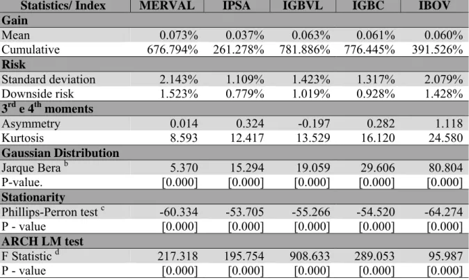
Table 1 shows the main descriptive statistics for the indices. Throughout the sample period, the Argentinian index accumulated a net gain of 676.79%, while the IPSA showed a gain of only 261.28%. The MERVAL had the highest standard deviation and the highest average daily return among the analyzed indices, but its performance, according to the Sharpe ratio, was similar to that of the Chilean index.

Table 2.1 – Summary statistics and violation tests applied to returns on South American stock market indices a

Statistics/ Index MERVAL IPSA IGBVL IGBC IBOV

Gain

Mean 0.073% 0.037% 0.063% 0.061% 0.060%

Cumulative 676.794% 261.278% 781.886% 776.445% 391.526%

Risk

Standard deviation 2.143% 1.109% 1.423% 1.317% 2.079%

Downside risk 1.523% 0.779% 1.019% 0.928% 1.428%

3rd e 4th moments

Asymmetry 0.014 0.324 -0.197 0.282 1.118

Kurtosis 8.593 12.417 13.529 16.120 24.580

Gaussian Distribution

Jarque Bera b 5.370 15.294 19.059 29.606 80.804

P-value. [0.000] [0.000] [0.000] [0.000] [0.000]

Stationarity

Phillips-Perron test c -60.334 -53.705 -55.266 -54.520 -64.274

P - value [0.000] [0.000] [0.000] [0.000] [0.000]

ARCH LM test

F Statistic d 217.318 195.754 908.633 289.053 95.987

P - value [0.000] [0.000] [0.000] [0.000] [0.000]

Notes: a Panel containing daily time series of nominal net returns on major stock exchanges in Latin America countries from 1998 to 2013. (4118 observations); b Jarque-Bera test for series normality, the test statistics measure the difference between skewness and kurtosis of the series with a normal distribution under the null hypothesis that the series follows a normal distribution; c_{Phillips-Perron unit root test, at a level with constant}

and trend, spectral estimation method Default (Bartlett Kernel); d Engle’s ARCH LM Test, the "Lagrange multiplier" type, for the hypothesis of residuals from ARMA models returns having an ARCH structure, under the null hypothesis that there is no ARCH with a lag. Null Hypothesis: There is no ARCH effect.

(32)

All the indices, except for the IGBVL, showed asymmetry to the right, with this being more pronounced for the IBOVESPA and less pronounced for the MERVAL.

All the indices feature leptokurtosis, since they show a kurtosis greater than the normal distribution, which is 3, and the magnitude is greatest for the Brazilian index and lowest for the Chilean one. This evidence suggests a priori the non-normality of the index return series. In this sense, with the aim of verifying the Gaussian nature more properly, the Jarque-Bera test was used; the result of this test indicates the rejection of the null hypothesis

of normality for all the series at a 1% level of significance. According to Mahadeva and Robinson (2004), the biggest problem of using regression models when there are non-stationary variables is that the standard error obtained is biased. Non-non-stationary series are not suitable if the final purpose is to make predictions, as they have little practical value because the behavior of the series is conditional on time. To examine whether the series are stationary, the Dickey and Fuller (1979) unit root test, in its augmented version, also known as the ADF test, was performed, and also the Phillips and Perron (1988) test. According to Mahadeva and Robinson (2004), the Phillips and Perron test (1988) is used as an alternative to the ADF test because, being a non-parametric test, it has advantages in various applications.

Thus, it was verified that for all the series, at a 1% significance level in both tests, the null hypothesis of the presence of a unit root is rejected; this is expected in returns seriesAlso, in order to determine whether or not there is heteroscedasticity to be modeled in the residues, Engle’s ARCHLM test was performed, and the results are shown in Table 1. It can be seen that for all series, at a 99% confidence level, the null hypothesis of the homoscedasticity of the residues is rejected. According to Engle (2001), in the presence of heteroscedasticity the regression coefficients estimated by the ordinary least squares method remain unbiased, but they give a false sense of precision. Engle (2001) argues that the autoregressive conditional heteroskedasticity (ARCH) and Generalized Autoregressive Heteroskedasticity (GARCH) models treat heteroscedasticity as a variance to be modeled, instead of considering it as a problem to be fixed.

(33)

Figure 2.2 – Nominal net returns on South American major market indices a

a. IBOVESPA b. MERVAL

c. IPSA d. IGBVL

e. IGBC Source: CMA Trade

Notes: a Daily series of nominal net return obtained from the time series closing price (end-of-day) of the indices in question during the period from January 07, 1998 to December 31, 2013, 4,118 observations.

It can also be seen that the Colombian index shows turbulence even before the crisis, with the largest negative peaks in June 2006. The Argentinian index has its most turbulent period in 2002.

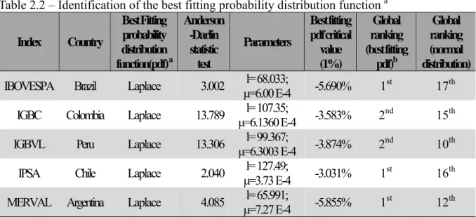
Finally, Table 2 reports the initial ranking positions in terms of the fitting of a wide range of distribution functions for the probability present, using the EasyFit software. It

-20% -10% 0% 10% 20% 30%

jan-98 jan-00 jan-02 jan-04 jan-06 jan-08 jan-10 jan-12

-15% -10% -5% 0% 5% 10% 15% 20%

-10% -5% 0% 5% 10% 15%

-15% -10% -5% 0% 5% 10% 15%

-15% -10% -5% 0% 5% 10% 15% 20%

(34)

is not exactly surprising that the normal distribution does not perform very well in the fitting rankings reported in this table. It can be observed that, in the aggregate ranking that considers the more than 50 continuous distributions that make up the Easy database, the normal distribution occupies positions like 10th and 17th, with the best distributions being identified as the Laplace for the Brazilian, Chilean and Argentinian indices. The best distribution for the Peruvian and Colombian indices is the Johnson SU.

Table 2.2 – Identification of the best fitting probability distribution function a

Index Country

Best Fitting probability distribution function(pdf) a

Anderson -Darlin statistic test Parameters Best fitting pdf critical value (1%) Global ranking (best fitting

pdf) b

Global ranking (normal distribution)

IBOVESPA Brazil Laplace 3.002 _μl= 68.033;

=6.00 E-4 -5.690% 1

st

17th

IGBC Colombia Laplace 13.789 _μl= 107.35;

=6.1360 E-4 -3.583% 2

nd

15th

IGBVL Peru Laplace 13.306 l= 99.367;

μ=6.3003 E-4 -3.874% 2

nd

10th

IPSA Chile Laplace 2.040 _μl= 127.49;

=3.73 E-4 -3.031% 1

st

16th

MERVAL Argentina Laplace 4.085 _μl= 65.991;

=7.27 E-4 -5.855% 1

st

12th

Notes: a The best-fitting pdf is identified and the ranking is done based on Anderson and Darling (1952) statistic. Our search for this specific and idiosyncratic distribution needs to impose a limitation on the range of continuous distribution families, because we can only use pdf's in which the standard deviation and the mean are given by univariate bijection, i.e., each moment depends on only one pdf parameter. b This is an unrestricted ranking, considering all continuous timing distributions.

Thus, for only these two indices, among the subset of distributions that can establish the bijection necessary for the quantile function to have a time-varying mean and standard deviation as arguments, it is noted that the Laplace function, which occupies second place in the overall ranking, presents the most appropriate fitting. Other distributions that satisfy this condition and have adequate fitting for the sector indices and for shares in the Brazilian capital markets are the logistic distribution and the secant hyperbolic distribution, among others.

2.4.3 Results: ARMA-GARCH

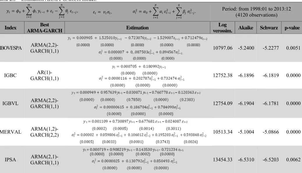
Based on Table 3, the series have different specifications, both in terms of the

(35)

Table 2.3 – Estimation ARMA-GARCH model.

Period: from 1998:01 to 2013:12 (4120 observations)

Index Best

ARMA-GARCH Estimation

Log

verossim. Akaike Schwarz p-value

IBOVESPA

ARMA(2,2)-GARCH(1,1) 10797.06 -5.2400 -5.2277 0.0051

IGBC

AR(1)-GARCH(1,1)

12752.38 -6.1896 -6.1819 0.0000

IGBVL

ARMA(2,2)-GARCH(1,1)

12754.09 -6.1904 -6.1781 0.0000

MERVAL

10513.34 -5.1004 -5.0866 0.0000

IPSA

13454.33 -6.5310 -6.5203 0.0062

Notes: a_{ARMA models estimated via OLS using the Newey-West coefficient for heteroscedasticity.}b_{ARMA-GARCH models estimated via ARCH, with normal errors}

distribution (Gaussian), using the Bollerslev-Wooldridge covariance coefficient for heteroscedasticity.

(36)

The parameters of the models estimated for the IBOVESPA, IGBC and IPSA indices are individually significant, even at the 1% level, both in the ARMA specification and in the GARCH framework. The IGBVL index obtained some parameters that were individually insignificant even at the 10% significance level in the ARMA specification, but the estimated GARCH parameters showed no problem with individual significance, even at the 1% level. However, the estimated model for the MERVAL presented a problem of individual significance in some parameters, for both the ARMA specification and the GARCH

framework.

Still considering Table 3, the p-value of the F statistic for the estimated ARMA-GARCH models is reported. The results demonstrate, in all the models estimated, that the null hypothesis that the slope coefficients of the estimated equations are jointly statistically insignificant is rejected at a 99% confidence level. Thus, the F-test confirms that the estimated models can be used to represent the return series of the South American indices for both the models estimated for the IGBVL and MERVAL indices, which showed some individual insignificant parameters, as well as for the other indices. The GARCH models obtained, except for the Argentinian index, are aligned with the results of Ferreira (2013), who states that “financial series are often better adjusted to low order GARCH models, with GARCH (1.1) being a very popular choice.”

2.4.4 Results: joint estimation

As a result of the contagion and financial integration for the main market indices in South America highlighted in Matos, Siqueira, and Trompieri (2014), it is intuitively clear that there can be benefits in risk modeling when considering the cross-effects in estimating the ARMA-GARCH frameworks. This happens through the joint estimation of this framework, that is, by using a multivariate GARCH of the AGDCC type (Asymmetric Generalized Dynamic Conditional Correlation). Theoretically, this framework accommodates

all the major criticism of the unconditional Gaussian VaR used in most parametric approaches to risk management.

(37)

greatly within the univariate and multivariate frameworks. In short, it is possible to observe a pattern of an inferior envelope being provided by the Laplace Multivariate Conditional VaR, with more extremes, that is, with an excess of conservatism that apparently provides a model with fewer exceptions.

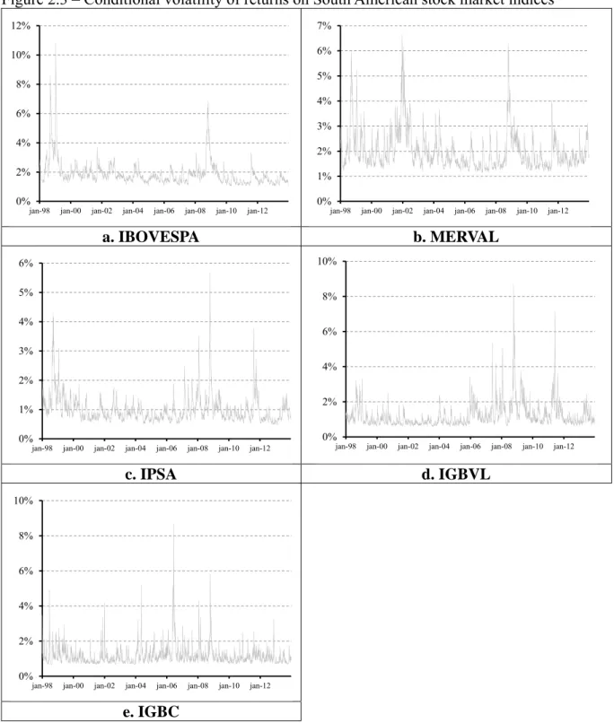
Figure 2.3 – Conditional volatility of returns on South American stock market indices a,b

a. IBOVESPA b. MERVAL

c. IPSA d. IGBVL

e. IGBC Source: CMA Trade.

Notes:a Daily series of nominal net return obtained from the time series closing price (end-of-day) of the indices in question during the period from January 07, 1998 to December 31, 2013, 4,118 observations. b One-step-ahead prediction performed using the ARMA-GARCH models estimated jointly.

0% 2% 4% 6% 8% 10% 12%

0% 1% 2% 3% 4% 5% 6% 7%

0% 1% 2% 3% 4% 5% 6%

0% 2% 4% 6% 8% 10%

(38)

2.4.5 Results: validation of models through backtesting

Aiming to analyzing cross-effects due to contagion and integration, in Graph 4 we plot the time evolution of the VaR series generated by following the multivariate metric, with a confidence level of 99% and a horizon of one day, as well as the daily return series for each banking index. Visual analysis allows us to suggest that, for all series, the maximum expected losses predicted by the multivariate VaR are closer to the realized losses than those predicted

by the base VaR.

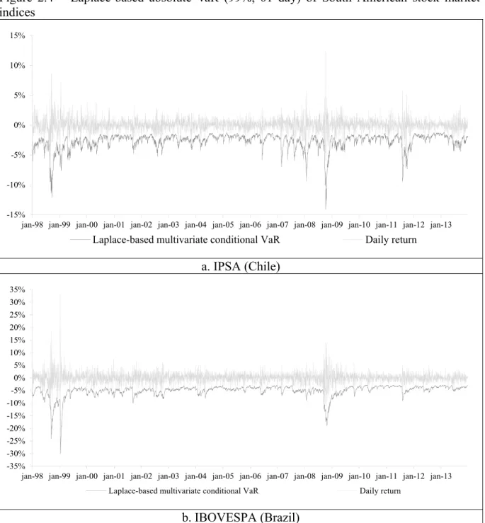
Figure 2.4 – Laplace-based absolute VaR (99%, 01 day) of South American stock market indices

a. IPSA (Chile)

b. IBOVESPA (Brazil)

Continue -15%

-10% -5% 0% 5% 10% 15%

Laplace-based multivariate conditional VaR Daily return

-35% -30% -25% -20% -15% -10% -5% 0% 5% 10% 15% 20% 25% 30% 35%

(39)

Continuation Figure 2.4 – Laplace-based absolute VaR (99%, 01 day) of South American stock market indices

c. IGBC (Colombia)

d. MERVAL (Argentina)

Continue -25%

-20% -15% -10% -5% 0% 5% 10% 15% 20%

Laplace-based multivariate conditional VaR Daily return

-20% -15% -10% -5% 0% 5% 10% 15% 20%

(40)

Conclusion Figure 2.4 – Laplace-based absolute VaR (99%, 01 day) of South American stock market indices

e. IGBVL (Peru)

Source: CMA Trade

According to Graph 4, there are three moments for all the South American markets when the highest values of VaR are seen, and these match the times of greatest volatility: i) the first half of 2009, still reflecting the subprime crisis in the United States; ii) the first half of 2010, as a result of a time of instability in the euro zone due to the first signs of the sovereign debt crisis; and iii) the second half of 2011, with the emergence of the same crisis signaling the possibility of some government defaults. Our purpose is to draw inferences about the relevance of contagion and financial integration effects between the South American stock market indices, and therefore multivariate conditional best-fitting VaR, which incorporates these cross-effects, is compared with the corresponding univariate version.

These models are similar in all aspects, except for the conditional moments incorporated into the distribution with the better fitting, which, in the latter VaR, are estimated from a univariate ARMA-GARCH, instead of a multivariate framework. To continue this comparison we must use the backtesting methods defined in the previous section. We report the results of the proposed backtesting in Table 4.

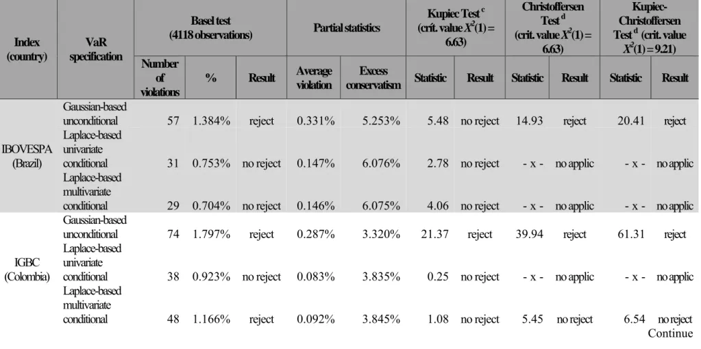
Using Basel backtesting, which takes into account violations in the absolute or relative amounts over the 4,118 daily observations, we reject Basel VaR for all economies, while univariate VaR is rejected for Argentina. Multivariate VaR fails for Colombia, Argentina, and Peru. For all the economies, the number of violations is higher for Basel VaR than for

-25% -20% -15% -10% -5% 0% 5% 10% 15%

(41)

univariate or multivariate VaR. Using backtesting that takes into account the frequency and conditionality of losses exceeding the VaR (the tests proposed by Kupiec (1995) or Christoffersen (1998) or the joint test proposed by these authors), while Basel VaR is rejected for all five economies, we fail to reject univariate conditional best-fitting VaR for all markets, while the multivariate version is rejected only for Peru and Chile. Since for most of the indices there are no successive violations when we use the univariate or multivariate VaR measures, we cannot measure a value for the statistical test proposed by Christoffersen (1998)

or for the joint test.

(42)

Table 2.4 – Backtesting methods applied to VaR of returns on South American stock market indices

Index (country)

VaR specification

Basel test

(4118 observations) Partial statistics

Kupiec Test c (crít. value X2(1) =

6.63)

Christoffersen Test d (crit. value X2(1) =

6.63)

Kupiec-Christoffersen Test d (crit. value

X2(1) = 9.21) Number

of violations

% Result Average violation

Excess

conservatism Statistic Result Statistic Result Statistic Result

IBOVESPA (Brazil)

Gaussian-based

unconditional 57 1.384% reject 0.331% 5.253% 5.48 no reject 14.93 reject 20.41 reject

Laplace-based univariate

conditional 31 0.753% no reject 0.147% 6.076% 2.78 no reject - x - no applic - x - no applic

Laplace-based multivariate

IGBC (Colombia)

Gaussian-based

unconditional 74 1.797% reject 0.287% 3.320% 21.37 reject 39.94 reject 61.31 reject

conditional 48 1.166% reject 0.092% 3.845% 1.08 no reject 5.45 no reject 6.54 no reject

(43)

Continuation Table 2.4 – Backtesting methods applied to VaR of returns on South American stock market indices a,b

Index (country)

VaR specification

Basel test

(4118 observations) Partial statistics

Kupiec Test c (crít. value X2(1) =

6.63)

Christoffersen Test d (crit. value X2(1) =

6.63)

Kupiec-Christoffersen Test d (crit. value

X2(1) = 9.21) Number

of violations

% Result Average violation

Excess

conservatism Statistic Result Statistic Result Statistic Result

MERVAL (Argentina)

Gaussian-based

unconditional 74 1.797% reject 0.383% 5.414% 21.37 reject 6.28 no reject 27.65 reject

conditional 46 1.117%

reject

0.170% 6.276% 0.55

no reject 0.37 no reject 0.92 no reject Laplace-based multivariate

reject

0.183% 6.271% 0.19

no reject 0.46 no reject 0.65 no reject IGBVL (Peru) Gaussian-based

unconditional 78 1.894% reject 0.348% 3.587% 26.34 reject 47.62 reject 73.96 reject

no reject

0.104% 4.134% 0.25

no reject

x

-no applic

- x -

no applic

reject

0.131% 4.139% 0.35