A self-adaptive evolutionary fuzzy model for load forecasting problems
on smart grid environment
Vitor N. Coelho
a,f,⇑, Igor M. Coelho
d,f, Bruno N. Coelho
f, Agnaldo J.R. Reis
a,c, Rasul Enayatifar
a,
Marcone J.F. Souza
e, Frederico G. Guimarães
baGraduate Program in Electrical Engineering, Universidade Federal de Minas Gerais, Belo Horizonte, Brazil bDepartment of Electrical Engineering, Universidade Federal de Minas Gerais, Belo Horizonte, Brazil cDepartment of Control Engineering and Automation, Universidade Federal de Ouro Preto, Ouro Preto, Brazil dDepartment of Computer Science, State University of Rio de Janeiro, Rio de Janeiro, Brazil
eDepartment of Computer Science, Universidade Federal de Ouro Preto, Ouro Preto, Brazil fInstituto de Pesquisa e Desenvolvimento de Tecnologias, Ouro Preto, Brazil
h i g h l i g h t s
Novel hybrid self-adaptive forecasting model optimized using meta-heuristics. Real-time parameter optimization during the learning process.
GRASP solution generator guided by values from feature extraction techniques. An expert mechanism for refining model’s inputs using a neighborhood structures. Results point out efficient MG load forecasting with low variability over MAPE.
a r t i c l e
i n f o
Article history:
Received 20 October 2015
Received in revised form 25 January 2016 Accepted 6 February 2016
Available online 23 February 2016
Keywords: Load forecasting Smart grids Microgrids Fuzzy logics
Hybrid forecasting model Parameter optimization
a b s t r a c t
The importance of load forecasting has been increasing lately and improving the use of energy resources remains a great challenge. The amount of data collected from Microgrid (MG) systems is growing while systems are becoming more sensitive, depending on small changes in the daily routine. The need for flex-ible and adaptive models has been increased for dealing with these problems. In this paper, a novel hybrid evolutionary fuzzy model with parameter optimization is proposed. Since finding optimal values for the fuzzy rules and weights is a highly combinatorial task, the parameter optimization of the model is tackled by a bio-inspired optimizer, so-called GES, which stems from a combination between two heuris-tic approaches, namely the Evolution Strategies and the GRASP procedure. Real data from electric utilities extracted from the literature are used to validate the proposed methodology. Computational results show that the proposed framework is suitable for short-term forecasting over microgrids and large-grids, being able to accurately predict data in short computational time. Compared to other hybrid model from the literature, our hybrid metaheuristic model obtained better forecasts for load forecasting in a MG scenario, reporting solutions with low variability of its forecasting errors.
Ó2016 Elsevier Ltd. All rights reserved.
1. Introduction
Electric grids are evolving from a centralized single supply model towards a decentralized bidirectional grid of suppliers and consumers. In this new environment, so-called Smart Grid (SG), the reality becomes a more dynamic scenario involving
uncer-tainty in energy production, consumption and distribution. The development of efficient algorithmic techniques that deal with these scenarios is crucial for supporting this important economical activity.
Rogers et al. [1] highlighted that the demand side, the con-sumers, will have to adapt to the available resources, in contrast to the current model in which the supply should always match the demand. In most countries, the starting point in the migration to this new business model and the implementation of the SG is the installation of smart meters[2]and sensors in residences and commercial buildings. The need for reducing environmental
http://dx.doi.org/10.1016/j.apenergy.2016.02.045 0306-2619/Ó2016 Elsevier Ltd. All rights reserved.
⇑ Corresponding author at: Department of Electrical Engineering, Federal Univer-sity of Minas Gerais, Belo Horizonte, MG 31270-010, Brazil. Tel./fax: +55 31 35514407.
E-mail addresses:[email protected],[email protected](V.N. Coelho).
Contents lists available atScienceDirect
Applied Energy
impacts, as emissions of greenhouse gases, lead to an increasing use of renewable energy systems (primarily wind and photovoltaic units)[3].
Considering measurement systems with high sampling rates over years of data acquisition[4], one can expect a large amount of detailed data. In case of electrical network metering, this data can be converted into valuable and useful information, which is crucial for the success of a wide range of SG applications. A task that has been left to the researchers is the one related to the selec-tion and analysis of parts of these datasets. From such data treat-ment, those huge datasets become available in different ways in order to allow researchers from distinct areas to develop smart solutions for multifunctional and highly complex problems.
Lee and Tong[5] underscore the importance of energy con-sumption forecasting in the context of economic development of a country due to the large and rapid changes in the industry, which have strongly affected energy consumption. Taylor and McSharry [6] emphasized that electricity demand forecasting is of great importance for the management of power systems. Nowadays, it is a consensuses that electrical load forecasting assisted by Artifi-cial Intelligence method plays a vital role for an effective success of the SG[7].
The need for Short-Term Load Forecasting (STLF) for controlling and scheduling of power systems is increasing, a task that is also required by transmission companies when a self-dispatching mar-ket is in operation. Commonly, in STLF studies one is interested in predictions for the next 1–24 h ahead samples in basis of half-an hour or one-hour[8]. Nowadays it is also possible to find research reporting shorter time periods, such as Guangui et al. [9], who studied wind power energy forecasting with 15 min of forecasting horizon. Furthermore, real-time forecasts will not be useful only for wind or solar forecasts, as it is already a need when considering Microgrids control and efficient management[10].
In terms of STLF, MG should be taken into account, since they are more difficult to be monitored and predicted than large power grids due to their higher randomness and lower autocorrelation factors[11]. MG had become a basic and fundamental infrastruc-ture in the SG environment and have been receiving attention in recent literature work. For instance, Zhi-Chao et al. [12] used a backpropagation neural network to perform forecasts over a MG environment, however, the accuracy of their results had been com-promised due to large load variations in the small office building that they had analyzed. A problem that generally does not happen in Large-Grid and Medium-Grid environments, as can be verified in Taylor and McSharry[6], where STLF was performed over a huge European data set from 10 different countries. As emphasized by Coelho et al.[13], forecasts and, in special, probabilistic forecasts will assist decision making in MG, guiding and assisting suitable and profitable energy storage. Forecasts of load and prices are also being considered for auction-based market, where the length of a market period has been modeled as an interval between 15 min and one hour, which is included in the category of STLF [14]. Hernández et al.[15] focus on Artificial Neural Networks (ANN) approach for STLF in order to provide useful information for MG intelligent elements, in case they can adapt their behavior depend-ing on the future generation and consumption conditions.
Recent works have proposed artificial intelligence techniques for dealing with load forecasting problems in applications where traditional forecasting methods have many limitations to tackle big data and higher load fluctuation[16], such as ANN[17], fuzzy inference systems (FIS) [18,19] and Fuzzy Times Series (FTS) [20,21], support vector machines (SVM)[22]and hybrid heuristic models[23,24].
Most forecasting models require feature extraction techniques in order to select good quality inputs[25]. Different works in the literature had already tried feature extraction for improving
fore-casting performance, specially for ANN[26]. Enayatifar et al.[21] obtained the Fuzzy Logical Relationships (FLRs) by analyzing the Autocorrelation Function (ACF). Recently, Lahouar and Slama[27] proposed the use of ACF to assist a mechanism for input selection of a random forecasting model. However, feature extraction from the time series is not the only viable solution to selecting possible sets of model’s inputs, this problem has been also approached with the use of bagging[28].
Driven by theoretical and real world applications, extracted from the literature and envisioned by the authors of this work, the purpose of our current paper is to use a class of bio-inspired metaheuristics for calibrating the parameters of a model based onif–thenfuzzy rules. We incorporated the power of the evolution-ary algorithms for optimizing the fuzzy rules and calibrating their parameters, while Neighborhood Strucutures – NS are used for searching for a prominent set of lags. The expert input selection done by the NS, along with the evolution process, modify and adjust the model inputs during the training phase. In this context,
Evolution Strategies– ES [29] stand out as a robust and flexible framework, which has been effectively applied for solving many combinatorial optimization problems[30,31], however, up to the moment, with only sparse/none results reported over forecasting problems. A hybrid heuristic algorithm based on Greedy Random-ized Adaptive Search Procedures – GRASP[32]and ES is proposed. The GRASP is used to generate the initial population of the ES pro-cedure. Each solution, initialized as a different forecasting model, is generated according to a randomized solution generator in connec-tion with a feature extracconnec-tion technique.
The need to develop high accurate models for energy consump-tion forecasting is imminent, starting from simple data mining and noise suppression methods to more complete and efficient machine learning algorithms. Grosman and Lewin[33]use an algo-rithm based on the concept of Genetic Programming – GP[34]to generate a prediction model for dynamic control with nonlinear assumptions. Kashid and Maity[35]proposes a model based on GP for summer monsoon rains forecasting across India territory. Vladislavleva et al.[36]perform a forecasting model for predicting power output of wind farms based on meteorological data, using a hybrid method, integrating symbolic regression with GP. Recently, Çelekli et al.[37]propose a hybrid model, combining ANN with Gene Expression Programming (GEP) [38], to a manufacturing metallurgy problem, involving the forecasting of sorption of an azo-metal.
However, MG can reveal additional problems and requirements for forecasting systems[11]: (1) compared to large power grid, the load of micro-grid is more difficult to forecast given the smaller capacity and higher randomness; (2) complex forecasting models would increase the requirement and cost on computational resources, leading to difficulty in application and promotion among users; (3) the relationship between load characteristics and the cor-responding forecasting accuracy lacks analysis and summary.
In addition, for ensuring forecasting accuracy of the proposed framework in real time systems, the use of metaheuristics based models offers flexibility for using the methodology on normal com-puters or embedded terminal devices. In view of the short demand of computational resources during the learning process, a real time update strategy is proposed, which represents an important advance for microgrid forecasts.
Dealing with load forecasting in different real databases, involving short-term forecasts on large grids and MG poses a great challenge. Thus, this paper tackles this issue by proposing a flexible open-source framework. The major contributions of this current work are:
Introduce a GRASP solution generator that selects inputs based on values from feature extraction techniques.
An expert mechanism for refining model’s inputs during the supervised learning phase using neighborhood structures, which can add, remove and adapt model’s input.
Minor contributions are related to:
Consider the use of different exogenous variables as input of the forecasting model, adapted or included during the evolutionary process.
Use of a bio-inspired optimizer based in the concepts of the ES. Apply the model over real load databases composed of different
typical MG consumers and large grids.
Quick training strategy for forecasting in online MG scenarios. Use of a metaheuristic based framework suitable to be applied
for different forecasting horizons, generating h-steps-ahead forecasting.
The remainder of this paper is organized as follows. Section2 provides a generic description of the load forecasting problems. Section 3 describes the proposed framework to tackle STLF. Section 4 presents the computational experiments, and, finally, Section5draws the final considerations and future work.
2. Load forecasting problems
The class of forecasting problems sought to be solved in this paper may be formulated as follows:
a set of time seriesTS¼ fy;z1;. . .;zeg, composed ofeþ1 differ-ent historical time series, including the variable of interest y
and, optional, exogenous variableszi8i2 ½1;e,
The target time seriesy¼y1;. . .;ytcomprises a set oft observa-tions; The optional set ofeexogenous time series is represented byzi¼ fzi
1;. . .zit;. . .ztþki eg;8i2 ½1;e.
The goal is to estimate the forecasts of a finite sequence f^ytþ1;. . .;^ytþkg, with kindicating the number of steps to be pre-dicted, namely forecasting horizon.
These steps ahead to be predicted are precisely following the sample timet, that is, the forecast are theksteps ahead starting fromtþ1 totþk. The vector of exogenous variables include infor-mation prior to time t and might also include predicted future pointstþh. It is even possible to haveke>k.
Finally, each predictable pointptcan be composed of combina-tions of lags from the target time seriesytand variableszit.
In this current study, we tackle load forecasting, which is a time series. Forecasting models are required to estimate its future evo-lution in terms of past samples and, eventually, being assisted by the use of some exogenous variables that affect the future load [27]. As an example of a time-series,Fig. 1depicts an hourly load historical data.
3. Methodology
In order to develop a flexible framework that could be applied to the different types of datasets, a new adaptive model is designed and described in this section. Section3.1 presents the proposed fuzzy model. Section 3.2 introduces how to represent the fuzzy rules into matrices, examples are given in Section3.1.2. Section3.3 describes the procedure of solution evaluation. Lastly, Section3.4 details the proposed algorithm for calibration of the fuzzy model rules and weights.
3.1. Fuzzy model
Initial ideas regarding to this proposed fuzzy model can be found in Coelho et al.[40,41]. This current work presents a more complete and general mathematical formulation of it.
Each input of the model ui;i¼1;. . .;r, with ui¼yðt xÞ;
ui¼zðt xÞorui¼zðtþxÞ, represents a choice for the composi-tion of lags that will be used to obtain the forecast, the backshift operators. For simplicity of the didactic description of the model, only lags from the target time seriesywill be stated in the math-ematical description of the fuzzy model. Thus, the model will only use lags provided by the historical time series y, being
ui¼yðt xÞ ¼yt x¼B x
yðtÞ, beingBthe lag operator or backshift for lagsxprior to timet.
For instance, two different lags can be selected as inputs,
u1¼yðt 24Þandu2¼yðt 1Þ, for forecasting a specific horizon
from the previously described sequence pðtÞ, with t 24 and
t 1, respectively.
Based on these inputs of the model, or even combination of them, the fuzzy rules are generated and described as follows:
if ui>~ai then fðtÞ ¼
v
i if ui<~bi then fðtÞ ¼wið1Þ
fori¼1;. . .;r. Each inputuiis associated with up to 2 inequalities. The rules are based on fuzzy inequality relations<~and>, which are~
described by fuzzy membership functions, and the parametersai andbi. The forecast value suggested by each rule is given by the parameters
v
iandwi. The main idea behind this model is to divide, in a fuzzy sense, each input into intervals. Whenever the input value is within a given interval, then the consequent of the rule con-tributes to the forecast value. New rules create new intervals and consequently more complex relationships between the inputs and the forecast output.Fig. 2exemplifies the effects of the rules. The first one,Fig. 2a, shows the effects of one rule for one input andFig. 2b introduces the notion of the fuzzy space when a new rule is added. These examples consider the use of a backshift operator yt x¼B
x
yðtÞ, for the input lagxprior to timet. Each fuzzy interval provides a dif-ferent weight for forecasting a given pointyt, given by the combi-nations of the weights
v
1;v
2;w1andw2.The fuzzy setAi¼ fx;
l
Ai>0jx2Xgrepresents the set of values that satisfy the inequalityui>~ai. The membership degree to this set is modeled by fuzzy membership functions, such as:l
Aiðui;ai;iÞ0; if ui6ai
i1þðui aiÞ
i ; if ai
i<ui6ai1; if ui>ai
8 > <
> :
ð2Þ
with
iP0.In a similar way, the fuzzy setBi¼ fx;
l
Bi>0jx2Xgrepresents the set of values that satisfy the inequalityui<~bi. The membership degree to this set is modeled by fuzzy membership functions, such as:l
Biðui;bi;
iÞ1; if uiPbi
1þðbi uiÞ
i ; if bi<ui6biþ
i0; if ui>biþ
i8 > <
> :
ð3Þ
with
iP0.The weight of each rule in the final forecast value depends on the membership degree of the inputuito the fuzzy set associated with that rule. The overall output of the model proposed in this paper is given by Eq.(4).
fðtÞ ¼X
r
i¼1 ^
l
AiðuiÞv
iþl
^BiðuiÞwi ð4Þwhere the parameters ai;bi;
i were omitted in the membership functions just to simplify the notation. Additionally:^
l
AiðuiÞ ¼l
AiðuiÞPr
i¼1
l
AiðuiÞ þl
BiðuiÞð5Þ ^
l
BiðuiÞ ¼l
BiðuiÞPr
i¼1
l
AiðuiÞ þl
BiðuiÞð6Þ
^
l
AiðuiÞandl
^BiðuiÞrepresent the strength of the rules in the forecast.Fig. 3exemplifies the effects of two pairs of rules with linear or sigmoid fuzzy rules. The same position depicted inFig. 2was kept for this example. As can be noticed, when a non-linear membership function was used the regression became smoother.
3.1.1. What’s the rationale?
The correlation between past lags and current observations has been studied for decades. Several models and analyses try to extract characteristics from the old lags and correlate them in order to achieve efficient forecasting models. For instance, the triv-ial random-walk[42], proposed more than 100 years ago, tries to face time series that show irregular growth by calculating the first differences. Plotting efficient and well-designed ACF and Partial Autocorrelation Function – PACF is still being researched, as can be checked in Hyndman[43].
Fig. 4shows a typical microgrid residence with maximum load of 273 KW, composed by the historical load time series and forecasts provided by an Autoregressive Integrated Moving Average – ARIMA[44]and Random Walk forecasting models.
The relationship between the lags and the output can provide useful information for designing the inputs that will be used by the forecasting model. The ACF describes the tendency for observa-tions made at adjacent time points to be related to one another.
a1 b1
v1 w1
input y t-x
f(y
t
)
(a) Effects of one rule for one input
a1 b2 b1 a2
w2 v1 w1 v2
input y t-x
f(y
t
)
(b) Effects of adding a new rule
a1 b2 b1 a2 w2
v1 w2 v2
input y t-x
f(y
t
)
(a) Rules with linear membership function
a1 b2 b1 a2
w2 v1 w2 v2
input y t-x
f(y
t
)
(b) Rules with sigmoid membership function
Fig. 3.Rules effects with linear and non-linear membership functions.
Forecasts from ARIMA(3,1,4) with drift
Time horizon
Microgr
id load (KW)
0 500 1000 1500 2000
50
100
150
200
250
(a) ARIMA
Forecasts from Random walk
0 500 1000 1500 2000
0
5
0
1
00
150
200
250
300
(b) Random-walk-without-drift
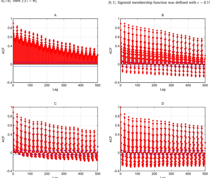
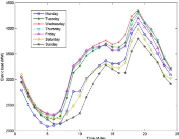
However, these correlations cannot be easily interpreted and adapted when time series with high fluctuations are dealt, such as loads from MG[16], wind power generation[45], wind speed [46], among others. For a better understanding of the ACF and results discussed in this section, the autocorrelation functions of four microgrids, described in Section4.2, are summarized inFig. 5.
3.1.2. Example
Suppose that after analyzing the most prominent inputs from an ACF, from a given time series (load, temperature, wind speed, etc.), the following inputs were selected to the model (the model can have repeated inputs, it is not a problem).
u¼
u1 u2 u3 u4 2
6 6 6 4
3
7 7 7 5
¼
yðt 1Þ
yðt 5Þ
yðt 40Þ
yðt 5Þ
2
6 6 6 4
3
7 7 7 5
Therefore, we have the following rules:
if u1>~a1 then fðtÞ ¼
v
1 if u1<~b1 then fðtÞ ¼w1ð7Þ
if u2>~a2 then fðtÞ ¼
v
2 if u2<~b2 then fðtÞ ¼w2ð8Þ
if u3>~a3 then fðtÞ ¼
v
3 if u3<~b3 then fðtÞ ¼w3ð9Þ
if u4>~a4 then fðtÞ ¼
v
4 if u4<~b4 then fðtÞ ¼w4ð10Þ
The forecast value is determined by the following equation:
fðtÞ ¼
l
^A1ðu1Þv
1þl
^B1ðu1Þw1þ
l
^A2ðu2Þv
2þl
^B2ðu2Þw2þ
l
^A3ðu3Þv
3þl
^B3ðu3Þw3þ
l
^A4ðu4Þv
4þl
^B4ðu4Þw4ð11Þ
Rule positions (aiandbi) and corresponding weights (
v
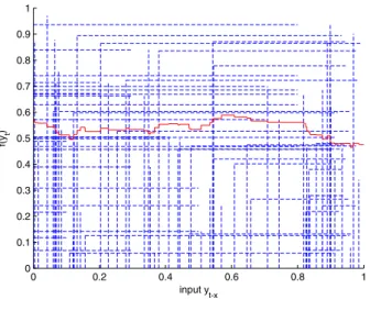
iandwi) are calibrated during the optimization process. In this current study, the weights and positions of the rules are calibrated accord-ing to an evolutionary metaheuristic algorithm. Additionally, the strategy is able to insert, remove and adapt rules during the train-ing process, as will be detailed in Section3.4.As a didactic example,Fig. 6depicts a defuzzification with 5 and 30 different pairs of fuzzy rules, using Heaviside step or sigmoid functions. Rules and weights were generated in the same interval ½0;1. Sigmoid membership function was defined with
¼0:15.0 100 200 300 400 500
-0.4 0 0.4 0.6 0.8 1
Lag
AC
F
A
0 100 200 300 400 500
-0.4 0 0.4 0.6 0.8 1
Lag
AC
F
B
0 100 200 300 400 500
-0.4 0 0.4 0.6 0.8 1
Lag
AC
F
C
0 100 200 300 400 500
-0.4 0 0.4 0.6 0.8 1
Lag
AC
F
D
3.2. Solution representation of the fuzzy rules
The following generic parameters describe the proposed model into a single matrix:
S¼
A
V
B
W
E 2
6 6 6 6 6 6 6 6 6 6 4
3
7 7 7 7 7 7 7 7 7 7 5
¼
a1 ar
v
1v
rb1 br
w1 wr
1 r2
6 6 6 6 6 6 6 6 6 6 4
3
7 7 7 7 7 7 7 7 7 7 5
ð12Þ
withi¼1;. . .;r.
Table 1illustrates a possible solution that uses four inputs over its model. The first two columns are related to values of a didactic load time series and the other two are inputs obtained from an associated temperature time series. Thus, in order to estimate a given forecast at timet, the model receives historical data from two different time series:
yðtÞ, which returns the values from a historical load time series. zðtÞ, exogenous variables which provide values from a
temper-ature time series.
and different lags:
yðt 1Þ and yðt 2Þ are the load consumption one and two hours before the forecasting (hour is used didactically to repre-sent a given discrete interval of data acquisition), respectively. zðt 1Þandzðt 24Þare the temperatures of the residence one
and 24 h before the desired forecasting.
0 0.2 0.4 0.6 0.8 1
0 0.1 0.2 0.3 0.4 0.5 0.6 0.7 0.8 0.9 1
input yt-x
f(y
t
)
(a) Five rules with sigmoid membership
functions
0 0.2 0.4 0.6 0.8 1
0 0.1 0.2 0.3 0.4 0.5 0.6 0.7 0.8 0.9 1
input yt-x
f(y
t
)
(b) Thirty rules with sigmoid
member-ship functions
0 0.2 0.4 0.6 0.8 1
0 0.1 0.2 0.3 0.4 0.5 0.6 0.7 0.8 0.9 1
input yt-x
f(
yt
)
(c) Thirty rules with Heaviside step functions
Fig. 6.Many rules effects with Heaviside and Sigmoid membership functions.
The first and the last inputs were modeled as triangular fuzzy rules, since both columns have
>0.Values used in this example stated byTable 1were arbitrarily chosen. Temperature values are used only didactically to empha-size the flexibility of the model in handling inputs from different time series. Brief results related to this mechanism are described in Section4.4.2.
3.3. Objective function and solution evaluation
A solutionsis evaluated by its ability of forecasting values of the training setT, comparing its forecasts with the historical mea-sured ones.
Most models are trained to minimize the Mean Squared Error (MSE), since it is well-known that the mean of the forecast distri-bution is obtained by minimizing the squared error loss function
Sð^yðtþhÞ;yðtþhÞÞ ¼ ð^yðtþhÞ yðtþhÞÞ2, where ^yðtþhÞ is the point forecast andyðtþhÞis the current observation obtained in the horizonh. However, other loss functions are also able to lead to the forecast mean[47], this topic is still being investigated with new diagrams and conditions[48,49].
Furthermore, the objective function can be any desired quality indicator or even more than one, in case of multiobjective approaches. Different metrics for defining the accuracy of forecast-ing models have been discussed in the literature. In the 90’s, Makridakis[50]proposed a discussion of theoretical and practical application of some loss functions.
3.4. GES training algorithm
The proposed calibration algorithm, calledGES, which tackle the rules optimization, consists on the combination of the metaheuris-tic procedures Greedy Randomized Adaptive Search Procedures – GRASP[32]and Evolution Strategy – ES[29]. The pseudocode is outlined inAlgorithm 1.
Algorithm 1. GES
From the MS procedure, the construction phase was used to gener-ate initial forecasting models, as can be verified in the BMIR (Build Model Inputs and Rules) procedure, detailed inAlgorithm 2. The initial population of the algorithm (lines 1 to 6 ofAlgorithm 1)
con-sists in generating
l
individuals. Each individual is generated according to the BMIR procedure and is, usually, of a different fore-casting model from each other.Algorithm 2. BMIR
Variable
a
regulates the size of theRCL, name Restricted Candi-date Lags, an abstraction of the Restricted List of CandiCandi-dates in GRASP. That is, input lags that have low correlation values, according to the desired feature extraction technique, will not be considered to be inserted in the model (line 3 ofAlgorithm 2). We denote variablea
tswith subscripttsto emphasize the possibility of limiting different lags according to the historical time series that the rule will use. The feature extraction technique receives the current greedy limita
, the maximum oldest lag able to be used by the modelmaxLagand the historical data. Section4.3discusses the influence of the greedy limit using a didactic example with ACF. The historical time series data are stored in the datasetM. The number of time series is given by the variablenTimeSeries. Variablerindicates the number of rules (basi-cally, 2r) that will be initialized in the model of solutions. From lines 6 to 11 ofAlgorithm 2, each column of the initial solutionsreceives a random input from theRCL. A trivial solution generator would be a feature extraction technique that returns a vector with all possible lags from 1 tomaxLag, then, the model would receive a random input lag for its rules. Position and weights of each fuzzy rule are initialized in accordance with a normal distribution (line 10), centered atmeantswith standard deviation
r
ts. A special case for the weightsv
andwis that they are all initialized withmean1andr
1, i.e.ts¼1. It was defined like this because, as standard, the firsttime series is the target that we need to forecast (in this current study, load time series). The other ones are auxiliary time series, such as temperatures, wind speed, presence of people at home, etc. Fol-lowing this procedure, in average, all the solutions generated by this procedure can forecast the mean values of the target load time series.
Line 4 ofAlgorithm 1merges the solution sand the standard deviations matrixM. The matrixMis generated in connection with the size of the model ofs(as stated by Eq.(13)).
M¼
r
Ar
Vr
Br
Wr
E 26 6 6 6 6 6 4
3
7 7 7 7 7 7 5
¼
r
a1r
arr
v
1r
v
rr
b1r
brr
w1r
wrr
r
r2
6 6 6 6 6 6 4
3
7 7 7 7 7 7 5
withi¼1;. . .;r.
From now on, the following nomenclature is used:
indSis the solutions, the fuzzy model, codified in the indi-vidualind;
indMis the matrix with the standard deviation values, used to guide evolution of the population through the generations.
In line 11 ofAlgorithm 1the mutation procedure is activated by a random individual of the actual population. Eq.(14) describes how the mutation is done. Each cell of the matrixindMis updated with a normal distribution, centered at zero with standard devia-tion
r
update,Mrow;col Mrow;colþNð0;
r
updateÞ ð14ÞThe procedure ApplyMutation (line 12 of the Algorithm 1) is illustrated in Eq.(15). Each rule, indSij, actually its position and weights are updated according to a normal distribution centered at zero and with standard deviation obtained from the respective cell of the mutation matrixindMij.
ind¼
AþNð0;MrAÞ VþNð0;MrVÞ BþNð0;MrBÞ WþNð0;MrWÞ
EþNð0;MrEÞ
2
6 6 6 6 6 6 4
3
7 7 7 7 7 7 5
ð15Þ
Line 13 of theAlgorithm 1has the ability of mutating the model lag using the neighborhood structures described in Section 3.5. Each of the three Neighborhood Structure – NS have probabilities
pNS1;pNS2;pNS3of being applied for mutating model’s inputs.
Finally, the selection procedure (line 16 of theAlgorithm 1) can be any desired selection strategy, as long as the strategy returns a population with
l
individuals. The one used here is described as competitionðl
þkÞ, following the same notation of Beyer and Sch-wefel[29]. In this selection process there is competition between parents and offspring. Thus, thel
best individuals are selected among parents and offspring.3.5. Expert model input adjustment using neighborhood structures
Three different NS were designed in order to adapt model’s input during the training phase. A brief view of the movements is described below:
Change lag –NSCLðsÞ: This move increases or decreases in one unit the lag of columnx½x2 ½1;rof solutions.
Remove rule –NSRRðsÞ: This move deletes one column from solutions(if the solution has, at least,r>1).
Add rule –NSARðsÞ: This move consists in adding a new rule withlag2 ½1;maxLagfor the solutions, with the same proce-dure described forAlgorithm 2.
The whole of designing expert input selection mechanisms has been envisioned by different researches, a considerable part of them generates specific subsets of features to be evaluated. Several approaches, such as those based on ANN[27], usually, define pairs composed of inputs and outputs,Tt
training¼ ðxttraining;yttrainingÞ, being
yt
training the historical measured values from the time series and
xt
training a N-dimensional vector of exogenous variables for the tth
time instance of a given time series.
The features sets are analyzed according to different feature selection methods [51], based on traditional statistical methods or artificial intelligence and machine learning strategies. Using pre-pocessing analysis, a specific set of inputs is chosen and, then, machine learning algorithms, based on different learning para-digms, are applied over the datasets. However, are these features sets optimal for those models? Some works in the literature have been claiming a strategy that finds the ‘‘best” set of inputs, but, it sounds to be a further discussion to achieve an optimal set of lags for a given forecasting model.
On the other hand, our proposal handles with time series as a sequence instead of defining sets of pairs of exogenous variables and desired outputs. Thus, the inputs required by a given solution
sare only accessed when this solution is being evaluated regarding its performance in the training set. This strategy provides the tool of real-time inputs searching. The expert input selection strategy proposed in this paper allows the model to be updated in any stage of the learning process, that is done using a metaheuristic procedure.
4. Computational experiments
This section is divided into five subsections. Section4.1presents the computational resources, some considerations about the code and model parameters. Section 4.2 introduces the real datasets used in this paper. Section4.3presents the results related to model inputs selection. Section4.4presents some results compared with the literature. Finally, Section 4.5presents results of our hybrid fuzzy model, applied in real-time MG load forecasting scenario, compared with well-known forecasting models.
4.1. Basic configurations
The GES calibration algorithm was implemented in C++ with assistance from OptFrame (Available at http://sourceforge.net/pro-jects/optframe/) [52]. In general, frameworks are based on the researchers experience with the implementation of multiple meth-ods for different problems. This optimization framework has been successfully applied in guiding the implementation of neighbor-hood structures (see[53]). Souza et al.[54,55]employed OptFrame to solve an open-pit-mining problem and a large-scale multi-trip vehicle routing problem. It is important to point out that all code used in this research is, from this moment, available as an example on OptFrame core, as an open-source tool under GNU LGPL 3.0.
The tests were carried out on a OPTIPLEX 9010 Intel Core i7-3770, 3.408 GHZ with 32 GB of RAM, with operating system Ubuntu 12.04.3 precise, and compiled by g++ 4.6.3, using the Eclipse Kepler Release.
According to empirical calibration and parameters suggested by the literature[29,41], the size of the population,
l
, and number of offspring,k, generated in each generation were fixed:l
¼10 and k¼60, respectively. Initial values for the standard deviation matrixMwere chosen at random from½1;10andr
updatewas fixed to be 1. The fine tuning of these values is not presented here since the main focus of the batches of experiments is to discuss the load forecasting regarding to different set of inputs. The objective func-tion (Secfunc-tion3.3) to be minimized during the fuzzy rules calibra-tion process was chosen to be the Mean Absolute Percentage Error – MAPE quality indicator[50].4.2. Datasets
dataset composed with load and temperature time series (mea-sured in Fahrenheit) was obtained from the Global Energy Fore-casting Competition 2014 – GEFCOM2014[56].
Taylor and McSharry[6]dataset consists in intraday electricity demand measurements, from 10 European countries for the 30 week period from Sunday, 3 April 2005 to Saturday, 29 October 2005. It is made up with hour (5040 samples), and half-hour (10,080 samples) load demand acquisitions.
Liu et al.[11]dataset is composed of four different microgrid users data (composed of users from small residential areas, com-mercial buildings or factories). Instances A and B are the load of residential areas, C and D are the load of commercial buildings. The load time series from these four MG were divided into two dif-ferent sets:
2
3of the data (1368 samples) is used for training the model;
1
3of the data (672 samples) is used as blind validation, in a way
to evaluate the performance of the model after the GES rules calibration.
Several characteristic indices are extracted separately from the history time series of loads from these different databases, in the same way as Liu et al.[11].
Average values of the load for each day are calculated and com-pared to the maximum load of that day (Rmeasure). Large grids presented higher values, since the average is closer to the peak val-ues. Following the same reasoning, the minimum daily load rate (Rmin) is lower for the microgrids historical load data. The European load consumption presented similar behaviors for the analyzed characteristics. As can be seen in the last four lines of the Table, daily load variation over the temperature time series of the MG residence is similar to the load grid variation over large grids. On the other hand, difference between two adjacent days is much higher than in large grids and fluctuates as in MG systems.
4.3. Expert input selection
As an example, we present a solution generator based on the ACF as a feature extraction technique for assisting the choice of the model inputs. Other feature extraction techniques[57]could be adapted to our greedy randomized solution generation BMIR.
The goal is to compare the models generated using inputs with high ACF value and the ones generated at random (when
a
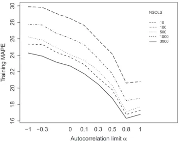
¼ 1). Model’s input should respect the maximum lagmaxLag. This first experiment intends to present the influence of ACF values for building an initial fuzzy model.Fig. 7indicates the MAPE errors of the best solution generated in ‘‘NSOLS” initializations.These experiments provide an initial insight about how building several initial solutions could enhance the chance of obtaining bet-ter initial models, in bet-terms of model’s performance measured by a MAPE indicator. This ability is reality in our approach due to the use of the GRASP procedure as the initial step of our training algorithm.
Model inputs are obtained from a given limit
a
which only con-sider lags with correlation higher than it, as introduced in Sec-tion 3.4. It should be noticed that we adapt the procedure for reducing the maximum lag until it reaches the input with maxi-mum lag value. For instance, if the given MG had the maximaxi-mum ACF value equal to 0.8, the results obtained witha
¼1 would be the same of those witha
¼0:8. However, as can be checked in ACF plots depicted in Fig. 5, the maximum ACF values of each MG have slightly different peak values.A second batch of experiment sought to analyze the behavior of different ACF limits
a
guiding the first initial population of the whole procedure. Additionally, we wanted to check if the expertself-adaptive input selection, using the NS described in Section3.5, might be able to mutate model’s lag, add and remove rules (as pointed in line 13 ofAlgorithm 1), during the training phase. The batch of experiment was composed of 4000 executions with learning time equal to two minutes. All the normality, independence and variance assumptions were verified and accomplished. The design of experiment was an effect model with different
a
¼ ½ 1; 0:3; 0:1;0:3;0:5;0:8;1, maximum number of rules maxNRules¼ ½10;100;500;1000, applied for learning the next step ahead of four different MG load time series (A, B, C, D). An Analysis of variance (ANOVA) test[58]was used for analyzing the differences between group means. The maximum lag (maxLag) was set to be 672. On the other hand, since the oldest lag used in the model of Liu et al. [11] was set to be 170 (set of inputs: ðzðt 1Þ;zðt 2Þ;zðt 22Þ;zðt 23Þ;zðt 24Þ;zðt 166Þ;zðt 167Þ;zðt 168Þ;zðt 169Þ andzðt 170ÞÞ), this same value will be fixed in the benchmark results of Section4.4.
Fig. 8depicts an interaction plot considering different
a
limits and the use of the expert input selection mechanism. Dashed lines show the variances of the model with and without the expert input selection. Best obtained models are depicted with points in shape of triangles. It can be noticed that when the model’s input was only determined by the BMIR, it improved the results whena
values were around 0:3, indicating that the model responded well for using input lag with low autocorrelation values. On the other hand, when the expert inputs adjustment was being used during the evo-lutionary process, the use of inputs with ACF values improved the training performance. The expert input selection strategy reduced the average MAPE errors from 13.9% to 12% for a two minutes training. By analyzing the dashed line it can be seen that the vari-ance of the model was also dramatically reduced by activating the self-adaptive mechanism.It was felt that the model might be able to reduce the training MAPE even when fed by inputs with low ACF value, if it has enough time for adjusting its parameters. Thus, inFig. 9we present the effects of the training time, TIMEES (seconds), using the proposed self-adaptive inputs selection strategy. Obtained results indicate the ability of the model in adjusting its input lag during long-runs training phases, an useful feature for long-term forecasting.
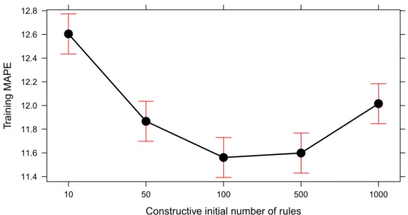
Regarding the number of the rules, the model performed better forecasts when initialized with a maximum number of rules equal to maxNRules¼100 or maxNRules¼500, as can be verified in Fig. 10. Thus, following some advices from the literature, we will
16
18
20
22
24
26
28
30
Autocorrelation limit α
T
raining MAPE
−1 −0.3 0 0.1 0.3 0.5 0.8 1
NSOLS
10 100 500 1000 3000
keep the constructive phase generating simpler models with an upper limit of 100 rules. Further studies should analyze if higher number of rules can result in model over-fitting, as already verified for FTS[21].
From now on, the constructive method will create initial models which have inputs with autocorrelation values greater than
a
¼0:5 andmaxNRules¼100 maximum rules.4.4. Benchmark results
The benchmark results are divided into three parts: Section4.4.1 presents the benchmark over the MG datasets; Section4.4.2shows the performance of the model in a case of study involving the use
5.0 7.5 10.0 12.5 15.0 17.5
−1 −0.3 −0.1 0 0.1 0.3 0.5 0.8 1
Autocorrelation limit α
T
raining MAPE
Expert input selection
no
yes
Fig. 8.Autocorrelation limita.
Constructive initial number of rules
T
raining MAPE
11.4 11.6 11.8 12.0 12.2 12.4 12.6 12.8
10 50 100 500 1000
Fig. 10.Effects of the initial number of rules and model’s performance.
789
1
0
1
1
Autocorrelation limit α
T
raining MAPE
−1 −0.3 0 0.3 0.5 0.8 1
TIMEES
120 1200 2400
load time series and temperature measurements; Section 4.4.3 indicates the results over the large grids.
4.4.1. Results over the MG datasets
The hybrid heuristic fuzzy model is compared with the EMD-EKF-KELM of Liu et al.[11]. Their model combines Empirical Mode Decomposition – EMD, Extended Kalman Filter – EKF, Extreme Learning Machine with Kernel – KELM and Particle Swarm Optimization – PSO. The forecasting horizon is one step ahead,
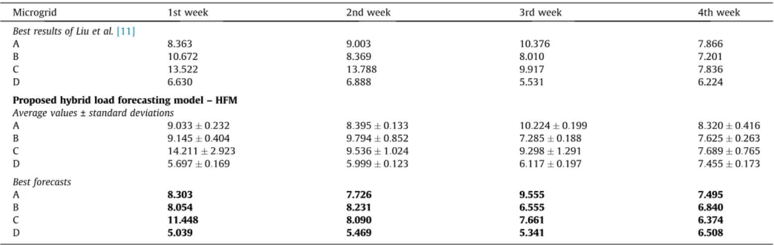
k¼1. MAPE and Root-Mean-Square Error – RMSE errors are pre-sented for each week of the validation set. A batch of 30 executions was done.Tables 2 and 3summarize the results of the new self-adaptive hybrid fuzzy model proposed in this paper compared to the EMD-EKF-KELM. The values in bold indicate the best values which are better than the best values of the EMD-EKF-KELM hybrid model, average values are not compared since they only reported the best achieved forecasts.
As can be verified inTables 2 and 3, the hybrid fuzzy model was able to obtain good mean results for both MAPE and RMSE quality indicators. Among the batch of 30 executions, at least one of the obtained model had better MAPE than the literature. For the RMSE, in four cases it was not able to achieve the best values reported by the literature.
Apart from the first week of the microgrid C, all other best results presented MAPE error lower than 10.25%. As described in
Liu et al.[11], it is known that when the MAPE is more than 10%, the operation cost of microgrids would increase sharply. If the obtained results were applied in real online situations, the archived forecasting errors would not lead to the sharp increase of operation cost, indicating that implementing the presented method over microgrid systems could bring benefits. Furthermore, the model was able to obtain good results with low variability, being the high standard deviation equal to 2.92%.
Another advantage of our approach is that it was competitive using one single set of parameters during the whole learning pro-cess. Liu et al.[11] divided the learning process in 48 groups of optimal parameters in workdays and holidays, obtained with an off-line parameter optimization using a PSO based algorithm. Here, we could do the same and trained 48 different models for each of their groups. For simplicity, and as a way of showing our model’s flexibility, we use only one single model with a single set of param-eters for each MG load time series.
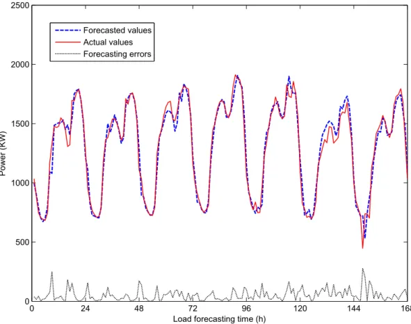
Fig. 11shows the forecast of the our best execution for the first week of the testing set. Forecasting errors are depicted in black dashed lines in the bottom of the figure, representing the absolute error between each prediction and the real value from the histori-cal time series.
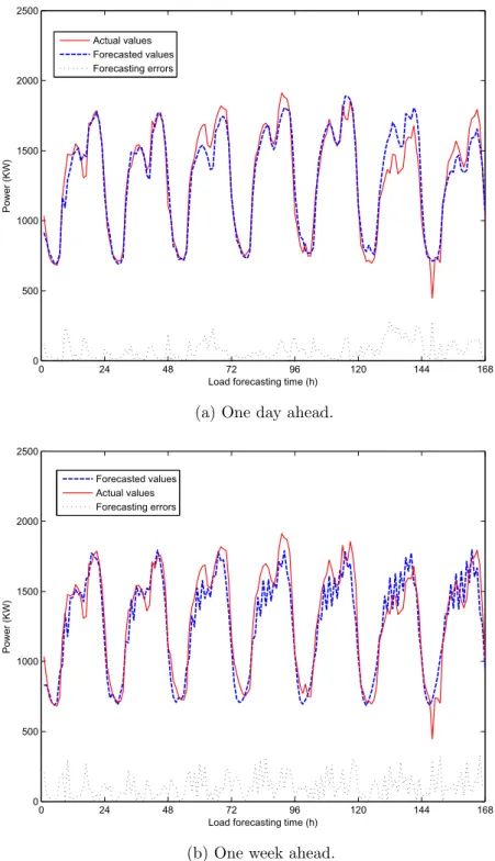
Finally,Fig. 12a and b depicts forecasts for one day and one week ahead.Fig. 12a indicates the forecasts for one day, over the first week of the validation set whileFig. 12b presents the forecasts
Table 2
Hybrid fuzzy modelEMD-EKF-KELM – MAPE (%).
Microgrid 1st week 2nd week 3rd week 4th week
Best results of Liu et al.[11]
A 8.363 9.003 10.376 7.866
B 10.672 8.369 8.010 7.201
C 13.522 13.788 9.917 7.836
D 6.630 6.888 5.531 6.224
Proposed hybrid load forecasting model – HFM Average values±standard deviations
A 9:0330:232 8:3950:133 10:2240:199 8:3200:416
B 9:1450:404 9:7940:852 7:2850:188 7:6250:263
C 14:2112:923 9:5361:024 9:2981:291 7:6890:765
D 5:6970:169 5:9990:123 6:1170:197 7:4550:173
Best forecasts
A 8.303 7.726 9.555 7.495
B 8.054 8.231 6.555 6.840
C 11.448 8.090 7.661 6.374
D 5.039 5.469 5.341 6.508
Table 3
Hybrid fuzzy modelEMD-EKF-KELM – RMSE (MW).
Microgrid 1st week 2nd week 3rd week 4th week
Best results of Liu et al.[11]
A 16.081 15.164 18.759 18.335
B 37.659 24.937 23.066 21.079
C 177.674 132.779 122.219 90.831
D 107.715 97.320 81.147 101.686
HFM
Average values±standard deviations
A 16:2360:452 14:0580:274 20:2990:659 17:8441:034
B 28:1925:122 29:9586:565 20:9391:989 23:1452:690
C 157:624100:669 95:77723:830 123:005185:266 88:48138:705
D 88:08131:545 91:98223:939 110:70746:645 124:82669:844
Best forecasts
A 15.204 13.162 18.932 16.456
B 24.411 25.954 19.059 20.548
C 144.491 88.355 104.616 76.621
for the whole first week ahead (k¼168). Even for one week ahead, the model was able to predict different slopes and load fluctuations over the analyzed MG.
4.4.2. MG forecasting with temperature measurements
A MG load historical data along with three different historical temperature time series, located in the surroundings of the MG, is considered in this section. As mentioned before, this historical dataset was obtained from the GEFCOM2014. The goal of this batch of experiment is to analyze fuzzy model’s performance towards the inclusion of new information from temperature time series.Fig. 13 exhibits the load autocorrelation function for this MG, with maxi-mum load of 325 KW, together with the autocorrelation for one of the temperature time series.
A batch of 30 executions with each of the four different combi-nation of exogenous variables as input of the model was performed.
Four different time series as input of the model: 1. only load historical data;
2. load data + one temperature time series; 3. load data + two temperature time series; 4. load data + three temperature time series.
The effect of the new temperature time series as input of the model can be seen inFig. 14a and b. Labels ‘‘1.Temp”, ‘‘2.Temp” and ‘‘3.Temp” refer to the use of the different historical tempera-ture time series. As can be verified, the proposed fuzzy model is able to handle with new information and can take profit of it in terms of optimizing model’s precision and performance. Average MAPE and RMSE decrease from 14.02% and 23.24% to 11.55% and
19.78%, respectively, when the three temperature time series were considered as model’s input.
Other time series could be included here and improvements could be expected, Tascikaraoglu and Sanandaji [59] recently detected an interesting trend between the data from a target house and the data from its surrounding houses. Following the same rea-soning of the experiment conducted in this section, new load time series from the surrounding MG could be included to be handled and enhance model’s forecasting performance.
Since the model is mainly based on metaheuristic it can be improved in order to use exogenous variables from different time series in some specific applications. The flexibility of the model and the use of NS makes the model suitable for real world applica-tions, since new structures can be design in order to change and adapt specific parts of the current model.
4.4.3. Results over the large grid datasets
Using the same set of parameters used for the MG, the model was applied to forecast load from large grids. For the European dataset of Taylor and McSharry[6], the first 20 weeks of each series were used to train the algorithm, the remaining ten weeks to eval-uate post-sample accuracy of 1–24 h ahead forecast.
A batch of 30 executions was done for each historical time ser-ies, average MAPE values are shown inTable 4.ELDhourly;ELDbeing the European Load Dataset, indicates the average MAPE for all the hourly historical time series (Italy, Norway, Spain and Sweden).
ELDhalfhourlyindicates the average MAPE for all the half-hourly
his-torical time series (Belgium, Finland, France, GB, Ireland and Portugal). All standard deviations were lower than 1.0% of MAPE.
The results presented inTable 4indicates that the model was also able to obtain average MAPE errors from 3.52% to 1.22% over
0 24 48 72 96 120 144 168
0 500 1000 1500 2000 2500
Load forecasting time (h)
Pow
er (KW)
Forecasted values Actual values Forecasting errors
the large-grid datasets. Compared to analyses made by Taylor and McSharry[6], the model also showed to be competitive.
4.5. Real-time online forecasting
In some applications, off-line learning is performed and, period-ically, re-trained if it is detected that the model is increasing its errors. This strategy was explored and detailed in the work of Liu et al.[11], updating their model if the MAPE increased more than a desired limit.
Since our proposal was able to obtain competitive results with two minutes training using low computational resources, we will
check the performance of the proposed model considering a real-time training strategy. This strategy is useful to overcome brutal changes in MG loads[27].
Furthermore, in future microgrids scenarios, the owner of the microgrid would take profit of the accuracy of the forecasting, since an efficient power dispatch will require precise schedules [60]. It is expected that it will be a reality not only for microgrid renewable energy generation, but also for MG users, which will do the best to train their models as the new data is available.
The concept of Number of Training Rounds (NTR), Eq.(16), gen-erates an important traded-off for forecasting models. NTR defines the number of samples used during the training phase related to a
0 24 48 72 96 120 144 168
0 500 1000 1500 2000 2500
Load forecasting time (h)
Power (KW)
Actual values Forecasted values Forecasting errors
(a) One day ahead.
0 24 48 72 96 120 144 168
0 500 1000 1500 2000 2500
Load forecasting time (h)
Pow
er (KW)
Forecasted values Actual values Forecasting errors
(b) One week ahead.
given forecasting horizonk. In the last experiments we used the NTR available from the literature, without checking if the use of less data during the training phase could improve the model’s
performance. It is an important aspect for understanding the behavior of the model with the size of the training set in a specific training time. The NTR is most frequently associated with the test-ing set error because it is known that the error of the traintest-ing set increases when the problem starts to learn big data problems. The Bias and Variance dilemma reinforces that increasing the training set size might provide more variability for the model for predicting information not seen before. On the other hand, the higher the NTR value is, the model requires more computational time to learn the historical load data.
Table 4
MAPE for the LG historical load time series.
Large power grid MAPE (%)
ELDhourly 3:5230:972
ELDhalfhourly 2:9830:621
0 24 48 72 96 120 144 168 192 216 240 264 288 312 336 360 384 408 432 456 480 500
-0.5 0 0.5 1
Lag
ACF
Sample Autocorrelation Function
0 24 48 72 96 120 144 168 192 216 240 264 288 312 336 360 384 408 432 456 480 500
-0.5 0 0.5 1
Lag
ACF
Fig. 13.Autocorrelation function for load and temperature of a small MG residence.
Input time series
MAPE
12.5 13 13.5 14 14.5
Load 1 Temp. 2 Temp. 3 Temp.
(a) Improvement on testing set MAPE
Input time series
RMSE
20.5 21 21.5 22 22.5 23 23.5
Load 1 Temp. 2 Temp. 3 Temp.
(b) Improvement on testing set RMSE
NTR¼#nTrainingSamples
k ð16Þ
Since MG requires quick response from the autonomous fore-casting agent[61], we run our experiment with ten seconds train-ing for different sizes of the traintrain-ing set. Fig. 15 shows an interactive plot of the NTR for the first week of the testing set of MG-A (red) and MG-C (blue). The points in shapes of triangles and crosses indicate respectively the minimum and maximum MAPE obtained in a batch of 10 executions. There are two types of lines representing each testing set, the dashed line indicates the standard deviation while the thicker line shows the average MAPE.
Finally, we compare our results with the methods ARFIMA[44], AUTO.ARIMA[44], Exponential Smoothing State Space model (ETS) [62], Naive Random Walk and trivial MEANF (historical mean of the training set). The AUTO.ARIMA uses a variation of the Hyndman and Khandakar[44]algorithm which combines unit root tests, minimization of the AICc and MLE to obtain an ARIMA model. For the automatic ARFIMA, auto-arima combined with a Fractionally-Differenced ARIMA, we consider the parameters cali-brated through Haslett-Raftery, so-called ARFIMA-LS, and full MLE, denominated ARFIMA-MLE.
Table 5indicates average MAPE for some well-known forecast-ing models and the proposed hybrid load forecastforecast-ing model, abbre-viated as HFM.
As can be verified in Table 5, the proposed HFM model was competitive with the automatic ARFIMA-LS, ARFIMA-MLE, AUTO. ARIMA, ETS and, as expected, trivial models naive RW and MEANF, reporting lower average MAPEs.
Since this model is mainly based on a metaheuristic calibration algorithm, it can be useful in real world applications that requires quick training, like the two minutes training performed in this last experiment. Furthermore, an intrinsic relationship with expected improvements on the metaheuristics quality will also enhance the performance of our training strategy.
5. Conclusions and extensions
5.1. Summary and final considerations
In this paper, a class of forecasting problem with realistic assumptions in Smart Grid scenarios was discussed. Despite its practical relevance, these variants of forecasting had received little attention of hybrid models based on metaheuristic. Because of its difficulty and large number of different forecasting scenarios in a future Smart Grid (SG) environment, a new flexible framework for forecasting was proposed.
This new approach consisted on a novel self-adaptive fuzzy model bio-inspired by Evolution Strategies to calibrate its parame-ters and model’s input. A smart solution generated based on the 0
5 10 15 20 25
1 3 6 12 24 168 336 672
Number of training rounds
T
esting MAPE − First w
eek
MG time series
0 3
Fig. 15.Number of training rounds with two minutes training.
Table 5
MG results with real-time online forecasting.
Microgrid k¼1 k¼24 k¼168 k¼672
672 336 168 24
First week of the testing set of MG-A
ETS 9.926 9.705 9.701 9.792
AUTO.ARIMA 10.030 9.982 9.606 10.344
ARFIMA-LS 9.890 9.774 9.768 10.064
ARFIMA-MLE 9.862 9.775 9.822 10.145
RW 9.680 9.680 9.680 9.680
MEANF 22.614 18.597 18.646 18.574
HFM 7.996 7.933 8.456 11.588
First week of the testing set of MG-C
ETS 13.796 14.032 13.948 15.012
AUTO.ARIMA 14.063 13.465 15.547 15.936 ARFIMA-LS 14.047 14.037 14.829 15.819 ARFIMA-MLE 13.873 14.287 14.861 15.913
RW 13.804 13.804 13.804 13.804
MEANF 34.589 34.844 37.361 32.920
constructive heuristic GRASP based on feature extraction tech-niques. The calibration process, done by the GES algorithm was able to go through a large search space of solutions with several different fuzzy rules and weights. The expert input selection and adaptation using NS allows more compact forecasting model, smal-ler training sets and easier training. Consequently, our new pro-posed model represents a step forward in determining a general procedure for input variable selection.
Real databases provided by Liu et al. [11], the Global Energy Forecasting Competition 2014 – GEFCOM2014 [56] and Taylor and McSharry[6] were used in order to verify the efficiency of the proposed model. It showed to be able to find good quality fore-casting models for microgrids and large-grids.
The methodology was able to obtain better results than the hybrid model of Liu et al.[11]. Particularly in view of the method’s flexibility, as it is mainly based on metaheuristics, it can be used in various everyday situations with minor adjustments.
A real-time microgrid forecasting scenario was also described and the model was compared with well-known forecasting models from the literature, presenting competitive results and lower MAPE for the analyzed historical MG time series.
5.2. Extensions
As future extensions for this work, the HFM could be adapted to tackle forecasting over different SG components, such as wind[63], solar[64]forecasting, smart park storage forecasting[65], among others.
Due to the nature of the model, mainly based onif–thenfuzzy rules, it is expected that it can be embedded in real world systems without a huge need of complex computational resources for per-forming the forecasting calculus.
The idea of handling with uncertainties when optimizing MG operation[66] motivates the possibility of analyzing the robust-ness of the proposed model in handling with variations over the model’s input. A given solution could be evaluated several times regarding the same historical time series with slight variations over its values. As recently done by Coelho et al. [13], a Sharpe Ratio index[67]could be designed for analyzing the performance of the proposed model when subjected to these uncertainties.
Valencia et al. [68] emphasized the ability of interval fuzzy models in providing a range rather than a trajectory. Thus, future works could also focus on checking if the same behavior can be obtained from our current proposed model.
Finally, a parallel version of GES would be very useful to improve the performance of the model in problems with a huge amount of data. This approach would take advantage of multi-core and GPU technology that is already present in current machines and with easy abstraction for heuristic algorithms.
Entire code used in this research is, from this moment, available as example on the OptFrame website. Thus, it is expected that future researchers continue contributing to enhancing the pro-posed model, increasing its efficiency and improving the tools and ideas presented in this paper.
Acknowledgment
The authors are indebted to the seven anonymous reviewers for their constructive suggestions that have helped us improve the original manuscript. The authors would like to thank Brazilian agency CAPES, CNPq (Grants 305506/2010-2, 552289/2011-6, 306694/2013-1 and 312276/2013-3), FAPEMIG (Grants PPM CEX 497-13), for supporting the development of this work. Vitor N. Coelho is also grateful to Raphael Camargo and Sarah L. Oliveira for their motivation and reviews.
In particular, we would like to thank James W. Taylor, J. Zico Kolter and Matthew J. Johnson for providing part of the dataset used in this work. We also would like to thank everyone that helped Taylor and McSharry [6] on their work. The authors are grateful to a number of people and organizations for supplying the data. These include M. O’Mallley (University College Dublin, Ireland), S. Majithia (National Grid, U.K.), J. Toro (Transmarket, Spain), R. Pestana (REN, Portugal), M. Uusitalo (Fingrid, Finland), M. Sveen (Marked- skraft), S. Grillo (University of Genova, Italy), and national transmission system operators, including Eirgrid in Ireland, RTE in France, Elia in Belgium, and Terna in Italy. Finally, we appreciate the assistance given by the research group of Nian Liu.
References
[1] Rogers A, Ramchurn SD, Jennings NR. Challenges for autonomous agents and multi-agent systems research. In: Twenty-sixth AAAI conference on artificial intelligence (AAAI-12), Toronto, CA; 2012. p. 2166–72.
[2] McHenry MP. Technical and governance considerations for advanced metering infrastructure/smart meters: technology, security, uncertainty, costs, benefits, and risks. Energy Policy 2013;59:834–42. doi:http://dx.doi.org/10.1016/j. enpol.2013.04.048.
[3] Batista N, Melício R, Matias J, Catalão J. Photovoltaic and wind energy systems monitoring and building/home energy management using zigbee devices within a smart grid. Energy 2013;49(0):306–15. doi: http://dx.doi.org/10. 1016/j.energy.2012.11.002.
[4] Monacchi A, Egarter D, Elmenreich W, D’Alessandro S, Tonello AM. Greend: an energy consumption dataset of households in Italy and Austria. Available from: arXiv:1405.3100.
[5] Lee Y-S, Tong L-I. Forecasting energy consumption using a grey model improved by incorporating genetic programming. Energy Convers Manage 2011;52(1):147–52.http://dx.doi.org/10.1016/j.enconman.2010.06.053. [6]Taylor J, McSharry P. Short-term load forecasting methods: an evaluation
based on European data. IEEE Trans Power Syst 2007;22(4):2213–9. [7] Raza MQ, Khosravi A. A review on artificial intelligence based load demand
forecasting techniques for smart grid and buildings. Renew Sustain Energy Rev 2015;50:1352–72. doi:http://dx.doi.org/10.1016/j.rser.2015.04.065. [8]Javed F, Arshad N, Wallin F, Vassileva I, Dahlquist E. Forecasting for demand
response in smart grids: an analysis on use of anthropologic and structural data and short term multiple loads forecasting. Appl Energy 2012;96 (0):150–60. smart Grids.
[9]Gangui Y, Yu L, Gang M, Yang C, Junhui L, Jigang L, et al. The ultra-short term prediction of wind power based on chaotic time series. Energy Proc 2012;17, Part B(0):1490–6. 2012 international conference on future electrical power and energy system.
[10] Pascual J, Barricarte J, Sanchis P, Marroyo L. Energy management strategy for a renewable-based residential microgrid with generation and demand forecasting. Appl Energy 2015;158:12–25. doi:http://dx.doi.org/10.1016/j. apenergy.2015.08.040.
[11]Liu N, Tang Q, Zhang J, Fan W, Liu J. A hybrid forecasting model with parameter optimization for short-term load forecasting of micro-grids. Appl Energy 2014;129(0):336–45.
[12] Sun Z-C, Chen T-H, Lian K-L, Kuo C-C, Cheng I-T, Chang Y-R, et al. Study on load forecasting of an actual micro-grid system in taiwan. In: 2013 IEEE international symposium on industrial electronics (ISIE); 2013. p. 1–7. [13] Coelho VN, Coelho IM, Coelho BN, Cohen MW, Reis AJ, Silva SM, Souza MJ,
Fleming PJ, Guimaraes FG. Multi-objective energy storage power dispatching using plug-in vehicles in a smart-microgrid. Renew Energy 2016;89:730–42. doi:http://dx.doi.org/10.1016/j.renene.2015.11.084.
[14] Stadler M, Cardoso G, Mashayekh S, Forget T, DeForest N, Agarwal A, et al. Value streams in microgrids: a literature review. Appl Energy 2016;162:980–9. doi:http://dx.doi.org/10.1016/j.apenergy.2015.10.081. [15] Hernández L, Baladrón C, Aguiar JM, Carro B, Sánchez-Esguevillas A, Lloret J.
Artificial neural networks for short-term load forecasting in microgrids environment. Energy 2014;75:252–64. doi: http://dx.doi.org/10.1016/j. energy.2014.07.065.
[16]Amjady N, Keynia F, Zareipour H. Short-term load forecast of microgrids by a new bilevel prediction strategy. IEEE Trans Smart Grid 2010;1(3):286–94. [17]Reis A, Alves da Silva A. Feature extraction via multiresolution analysis for
short-term load forecasting. IEEE Trans Power Syst 2005;20(1):189–98. [18] Mastorocostas P, Theocharis J, Bakirtzis A. Fuzzy modeling for short term load
forecasting using the orthogonal least squares method. IEEE Trans Power Syst 1999;14(1):29–36.http://dx.doi.org/10.1109/59.744480.
[19] Wai R-J, Chen Y-C, Chang Y-R. Short-term load forecasting via fuzzy neural network with varied learning rates, in: 2011 IEEE international conference on fuzzy systems (FUZZ); 2011. p. 2426–31.
![Fig. 4 shows a typical microgrid residence with maximum load of 273 KW, composed by the historical load time series and forecasts provided by an Autoregressive Integrated Moving Average – ARIMA [44] and Random Walk forecasting models.](https://thumb-eu.123doks.com/thumbv2/123dok_br/15701136.629088/4.892.60.733.512.1073/microgrid-residence-composed-historical-forecasts-autoregressive-integrated-forecasting.webp)