❊♥s❛✐♦s ❊❝♦♥ô♠✐❝♦s
❊s❝♦❧❛ ❞❡
Pós✲●r❛❞✉❛çã♦
❡♠ ❊❝♦♥♦♠✐❛
❞❛ ❋✉♥❞❛çã♦
●❡t✉❧✐♦ ❱❛r❣❛s
◆◦ ✹✾✶ ■❙❙◆ ✵✶✵✹✲✽✾✶✵
❋♦r❡❝❛st✐♥❣ ❊❧❡❝tr✐❝✐t② ▲♦❛❞ ❉❡♠❛♥❞✿ ❆♥❛❧✲
②s✐s ♦❢ t❤❡ ✷✵✵✶ ❘❛t✐♦♥✐♥❣ P❡r✐♦❞ ✐♥ ❇r❛③✐❧
▲❡♦♥❛r❞♦ ❘♦❝❤❛ ❙♦✉③❛✱ ▲❛❝✐r ❏♦r❣❡ ❙♦❛r❡s
❖s ❛rt✐❣♦s ♣✉❜❧✐❝❛❞♦s sã♦ ❞❡ ✐♥t❡✐r❛ r❡s♣♦♥s❛❜✐❧✐❞❛❞❡ ❞❡ s❡✉s ❛✉t♦r❡s✳ ❆s
♦♣✐♥✐õ❡s ♥❡❧❡s ❡♠✐t✐❞❛s ♥ã♦ ❡①♣r✐♠❡♠✱ ♥❡❝❡ss❛r✐❛♠❡♥t❡✱ ♦ ♣♦♥t♦ ❞❡ ✈✐st❛ ❞❛
❋✉♥❞❛çã♦ ●❡t✉❧✐♦ ❱❛r❣❛s✳
❊❙❈❖▲❆ ❉❊ PÓ❙✲●❘❆❉❯❆➬➹❖ ❊▼ ❊❈❖◆❖▼■❆ ❉✐r❡t♦r ●❡r❛❧✿ ❘❡♥❛t♦ ❋r❛❣❡❧❧✐ ❈❛r❞♦s♦
❉✐r❡t♦r ❞❡ ❊♥s✐♥♦✿ ▲✉✐s ❍❡♥r✐q✉❡ ❇❡rt♦❧✐♥♦ ❇r❛✐❞♦ ❉✐r❡t♦r ❞❡ P❡sq✉✐s❛✿ ❏♦ã♦ ❱✐❝t♦r ■ss❧❡r
❉✐r❡t♦r ❞❡ P✉❜❧✐❝❛çõ❡s ❈✐❡♥tí✜❝❛s✿ ❘✐❝❛r❞♦ ❞❡ ❖❧✐✈❡✐r❛ ❈❛✈❛❧❝❛♥t✐
❘♦❝❤❛ ❙♦✉③❛✱ ▲❡♦♥❛r❞♦
❋♦r❡❝❛st✐♥❣ ❊❧❡❝tr✐❝✐t② ▲♦❛❞ ❉❡♠❛♥❞✿ ❆♥❛❧②s✐s ♦❢ t❤❡ ✷✵✵✶ ❘❛t✐♦♥✐♥❣ P❡r✐♦❞ ✐♥ ❇r❛③✐❧✴ ▲❡♦♥❛r❞♦ ❘♦❝❤❛ ❙♦✉③❛✱ ▲❛❝✐r ❏♦r❣❡ ❙♦❛r❡s ✕ ❘✐♦ ❞❡ ❏❛♥❡✐r♦ ✿ ❋●❱✱❊P●❊✱ ✷✵✶✵
✭❊♥s❛✐♦s ❊❝♦♥ô♠✐❝♦s❀ ✹✾✶✮
■♥❝❧✉✐ ❜✐❜❧✐♦❣r❛❢✐❛✳
Nº 491
ISSN 0104-8910
Forecasting electricity load demand: Analysis of the 2001
rationing period in Brazil
Leonardo Rocha Souza
Lacir Jorge Soares
Forecasting Electricity Load Demand: Analysis of the 2001 Rationing
Period in Brazil
Leonardo Rocha Souza
EPGE/ Fundação Getúlio Vargas
Lacir Jorge Soares
CEPEL e UENF.
Abstract. This paper studies the electricity load demand behavior during the 2001
rationing period, which was implemented because of the Brazilian energetic crisis. The hourly data refers to a utility situated in the southeast of the country. We use the model proposed by Soares and Souza (2003), making use of generalized long memory to model the seasonal behavior of the load. The rationing period is shown to have imposed a structural break in the series, decreasing the load at about 20%. Even so, the forecast accuracy is decreased only marginally, and the forecasts rapidly readapt to the new situation. The forecast errors from this model also permit verifying the public response to pieces of information released regarding the crisis.
1 – Introduction
Supplying electricity efficiently involves complex tasks. For example, short-term
planning of electricity load generation allows the determination of which devices shall
operate and which shall not in a given period, in order to achieve the demanded load at
the lowest cost. It also helps to schedule generator maintenance routines. The system
operator is responsible for the hourly scheduling and aims foremost at balancing power
production and demand. After this requirement is satisfied, it aims at minimizing
production costs, including those of starting and stopping power generating devices,
taking into account technical restrictions of electricity centrals. Finally, there must
always be a production surplus, so that local failures do not affect dramatically the
whole system.
It is relevant for electric systems optimization, thus, to develop a scheduling
algorithm for the hourly generation and transmission of electricity. Amongst the main
inputs to this algorithm are hourly load forecasts for different time horizons. Electricity
load forecasting is thus an important topic, since accurate forecasts can avoid wasting
energy and prevent system failure. The former when there is no need to generate power
above a certain (predictable) level and the latter when normal operation is unable to
withstand a (predictable) heavy load. The importance of good forecasts for the operation
of electric systems is exemplified by many works in Bunn and Farmer (1985) with the
figure that a 1% increase in the forecasting error would cause an increase of £10 M in
the operating costs per year in the UK. There is also a utility-level reason for producing
good load forecasts. Nowadays they are able to buy and sell energy in the specific
market whether there are shortfalls or excess of energy, respectively. Accurately
forecasting the electricity load demand can lead to better contracts. Among the most
important time horizons for forecasting hourly loads we can cite: one hour and one to
seven days ahead. This paper deals with forecasts of load demand one to seven days (24
to 168 hours) ahead for a Brazilian utility situated in the southeast of the country.
The data in study cover the years from 1990 to 2002 and consist of hourly load
demands. We work with sectional data, that is, each hour’s load is studied separately as
a single series, so that 24 different models are estimated, one for each hour of the day.
All models, however, have the same structure. Ramanathan et al. (1997) won a load
forecasting competition at Puget Sound Power and Light Company using models
individually tailored for each hour. They also cite the use of hour-by-hour models at the
ways, including that we use only sectional data in each model. Using hour-by-hour
models avoids modeling the intricate intra-day pattern (load profile) displayed by the
load, which varies throughout days of the week and seasons. Otherwise, modeling one
single hourly series would increase model complexity much more intensely than would
allow possible improvements in the forecast accuracy. Although temperature is an
influential variable to hourly loads, temperature records for the region in study are hard
to obtain and we focus our work on univariate time series modeling. This modeling
includes a stochastic trend, seasonal dummies to model the weekly pattern and the
influence of holydays. After filtering these features from the log-transformed data, there
remains a clear seasonal (annual) pattern. Analyzing the autocorrelogram, a
hyperbolically damped sinusoid is observed, consistent with a generalized long memory
(Gegenbauer) process, which is used to model the filtered series.
The period in study comprises the Brazilian 2001 energetic crisis, briefed as
follows. It is well known that hydroelectric plants constitute the main source of
electricity in Brazil. In the beginning of 2001, below-critical reservoir levels turned on a
red light to normal electricity consumption. An almost nationwide energy-saving
campaign was deflagrated and rationing scheme implemented. These have successfully
lowered the electricity load demand, without impacting too much the industrial
production. The post-rationing loads remained low, among other causes, because of an
increase in the energy price and improvements towards efficient use of energy.
Apparently, there is a structural break in the load time series. This break consists of a
smooth and steady decrease in consumption, during approximately two months,
triggered by the information released by the Brazilian government that there could be
compulsory electricity cut-offs if the rationing scheme would not achieve its aims.
Because of the structural break, we analyze separately the forecasts of years
2000, 2001 and 2002. While year 2001 shows loss of accuracy comparing to 2000, this
loss is not dramatic and is partly recovered in 2002, which incorporates in the estimated
model influences of the decrease in consumption. Considering the year 2000, for one
day (24 hours) ahead, the mean absolute percentage error (MAPE) varies from 2.6%
(21th hour) to 4.4% (2nd hour). For two days ahead, the range is from 3.3% (20th hour) to 6.5% (2nd hour). For seven days ahead, in turn, the MAPE does not increase too much, staying between 3.9% (20th hour) and 8.4% (2nd hour). On the other hand, considering the year 2001 (with rationing), the MAPE can be as low as 2.7% and as high as 4.1%
characteristics observed in the data and the results obtained in forecasting, we conclude
for the presence of generalized long memory characteristics in the data studied,
enduring even a structural break in the series level.
The plan of the paper is as follows. The next Section exposes the energetic crisis
Brazil faced in 2001, how it was overcome and what implications resulted from that.
Section 3 briefly introduces generalized long memory, while Section 4 explains the data
and presents the model used to forecast the loads. Section 5 shows the results and
Section 6 offers some final remarks.
2 –Brazilian energetic crisis
2.1 – Overview of the crisis
In most countries, energy investments are balanced on different kinds of energetic
sources, in order to avoid that problems specific to one type of generation affect to a
great extent electricity supply as a whole. Diversification decreases risk when negative
shocks are not highly correlated among the diverse options. However, in great part due
to the generosity of water volumes running within the country, the Brazilian energetic
matrix is highly dependent on hydroelectric power plants, which constitute 87% of the
total source of electricity. Hydroelectricity generation is in turn highly dependent on
climatic conditions, such as rainfalls. The remaining sources of electricity in Brazil
include thermoelectric (10%) and nuclear (2%) power plants.
The energetic crisis in Brazil was perceived in the beginning of 2001, when it
was announced that the reservoirs were filled on average with only 34% of their
capacity, while they should be at least half full in order to endure the dry season in
normal operation. This picture was true only for the central part of the country, while
the north had a slightly less unfavorable situation (the rationing scheme was delayed in
two months for this region) and the south, on the other hand, was spilling water from its
reservoirs. However, the continental dimension of the country, allied to a lack of
investments in high-capacity long transmission lines, make geographic regions
“electrically isolated” from each other.
This situation occurred mainly because of the lack of rains and of investments in
electricity generation and transmission. The former had achieved the lowest volume in
20 years, while the latter had decreased to a half in the nineties. As if it was not enough,
electricity consumption was sharply rising at a rate of about 5% a year since the first
started in the beginning of the second quarter of 2001, and in addition a rationing
scheme was implemented from June 4, 2001 to February 28, 2002, when technical
conditions allowed the restoration of normal consumption.
2.2 – Rationing scheme
The scheme consisted basically of establishing a target consumption (20% below the
average consumption observed in the same period of the previous year) for each
household, shop, industry or any other electricity consumer. Simplifying the rules,
people who consumed below this target (and below the threshold level of 200
kWh/month) would be rewarded with a bonus in the electricity bill, whereas those
consuming above the target would be overtaxed and face the risk of having the
electricity supply cut off for three days. The implementation of this latter feature was
deterred by technical and political difficulties and eventually no consumer had their
energy supply cut off. The campaign and the scheme were very successful in that the
consumption was decreased to a great extent, thanks to popular response and technical
work. Although consumption was expected to rise again after the rationing was ended, it
was not observed. Very successful measures such as bulb substitutions and change of
habits increased efficiency in the use of electricity and reduced its waste. Also, an
increase in the energy price, imposed by the government to compensate for income
losses faced by the utilities due to the rationing scheme, contributed for the demand to
remain at a lower level.
Another notable occurrence was that a expected decrease in the industrial
production during the rationing period was not observed, since industries stocked
products beforehand as they were afraid (or possibly aware) of the coming rationing,
and made efforts towards turning the use of electricity more efficient thereafter. It is
worthwhile noticing that the industries had already decreased their consumption at
12.2% on average, as approximately half of them had adopted measures of energetic
efficiency in the previous three years (CNI, 2001a). In so doing, they had then little
slack to meet the rationing requirements without decreasing their production. Creativity,
however, was almost an imposition and approximately ¾ of the major industries and ½
of the small and medium-sized ones invested on the reduction of energy consumption
from the system. Mostly they invested on new efficient capital goods, allowing reducing
2.3 – Important dates
This subsection displays dates which correspond to the arrival of new information to the
consumers on the energy market. Two other important dates, specifically the beginning
and the end of the rationing scheme, were offered in Section 2.1.
Although the possibility of implementing an electricity rationing scheme had
been announced at least as early as mid-March 2001, only in April 26 the National
System Operator (ONS) and the government confirmed that this scheme would be put in
practice. In the meanwhile, the government announces a plan for reducing electricity
consumption (April 5); the Minister of Energy goes on TV to ask people to save electric
energy (April 15); the government admits that a rationing scheme may be unavoidable
(April 24); and a survey from the National Confederation of Transports (CNT) reveals
that more than a half of the interviewed people believed real the possibility of a
rationing scheme (April 25). A key date, however, is May 3, 2001, when the
government announces that if the rationing scheme would fail to achieve its objectives,
compulsory electricity supply cut-offs could be implemented.
2.4 – Structural break?
This section shows why the announcement of the possibility of cutting off compulsorily
the electricity supply turned May 3, 2001 into a key date. Although the rationing
scheme would be implemented only one month later, the fear of a cut-off made people
start saving energy from May 4, 2001 on. The decrease on the consumption level
occurred smoothly, taking more than two months to reach a new steady state level, as
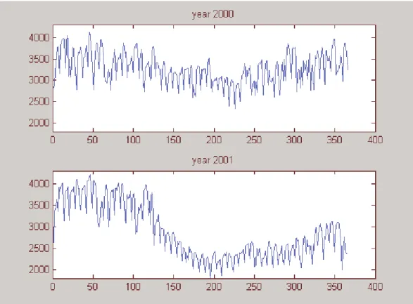
can be noticed in Figure 1. The smoothness of this break is understandable, since habits
are not changed instantly, and people do not change habits at the same time or the same
pace. Moreover, replacing old appliances by new efficient ones (e.g., incandescent bulbs
by fluorescent ones; old air-leaking fridges by new, sealed and more efficient ones) is
not an instantaneous process. Figure 1 compares the daily load between years 2000 and
2001, where one can notice by visual inspection the level downshift in the 2001 load,
occurring smoothly from the beginning of May (around May 4, the 125th day of 2001) to mid-July (around the 195th day of 2001). After that, the 2001 load seems to have incorporated this level downshift, following after its “usual seasonal pattern”.
Albeit successful the energy-saving campaign and the rationing scheme, the
positive response from the population posed a new problem. Electricity demand
forecasters face a structural break in the demand time series, hindering the forecasting
process. We show in this paper that the model proposed by Soares and Souza (2003)
rapidly readapts to the new data and achieves forecast error almost as low as the
formerly observed (before the rationing scheme). So, even with a structural break in the
series level, some statistical properties are not lost and are captured by the model.
3 – (Generalized) Long Memory
Long memory in stationary processes has traditionally two alternative definitions, one in
the frequency-domain and the other in the time-domain. In the frequency-domain, this
feature implies that the spectrum is proportional to a power of the frequency λ as λ
approaches zero. In the time-domain, the autocorrelations decay hyperbolically, instead
of geometrically as in ARMA processes. In both cases, d is the long memory parameter
and the above relationships characterize long memory and stationarity if d ∈ (0, 0.5).
Good reviews of long memory literature are found in Beran (1994) and Baillie (1996).
The specific frequency-domain definition is as follows. Let f(λ) be the spectral
density function of the stationary process Xt. If there exists a positive function cf(λ), ]
, ( π π
λ∈ − , which varies slowly as λ tends to zero, such that d ∈ (0, 0.5) and
0 as ) ( ~ )
(λ cf λ λ−2d λ→
f , (1)
then Xt is a stationary process with long memory with (long-)memory parameter d.
Alternatively, in the time-domain, let ρ( )k be the k-th order autocorrelation of the
series Xt. If there exists a real number d ∈ (0, 0.5) and a positive function c kρ( ) slowly
varying as k tends to infinity, such that:
2 1 ( ) ~k c k k( ) d as k
ρ
ρ − → ∞
(2)
then Xt is said to have long memory or long range dependence.
Hosking (1981) and Granger and Joyeux (1980) proposed at the same time the
fractional integration, which has no physical but only mathematical sense. It is
represented by a noninteger power of (1 – B), where B is the backward-shift operator
such that BXt = Xt-1, and can generate long memory while still keeping the process
stationary. The non-integer difference can be expanded into an infinite autoregressive or
moving average polynomial using the binomial theorem:
∞ = − = − 0 ) ( ) 1 ( k k d B k d
where ) 1 ( ) 1 ( ) 1 ( + − Γ + Γ + Γ = k d k d k d
and Γ(.) is the gamma function.
The fractional integration allows one to generalize the ARIMA processes, as
follows. Xt is said to follow an ARFIMA(p,d,q) model if Φ( )(B 1−B X)d t =Θ( )Bεt, where εt is a mean-zero, constant variance white noise process, d is not restricted to
integer values as in the ARIMA specification, and Φ(B)= 1-φ1B-…-φpBp and
Θ(B)=1+θ1B+…+θqB q
are the autoregressive and moving-average polynomials,
respectively. ARFIMA processes are stationary and display long memory if the roots of
Φ(B) are outside the unit circle and d ∈ (0, 0.5). If d < 0 the process is still stationary, but is short memory and said to be “antipersistent” (Mandelbrot, 1977, p.232), and
Equation (1) holds so that the spectrum has a zero at the zero frequency. Note that in
this case the process does not fit into the definition of long memory, since the parameter
d is outside the range imposed by this definition. If d = 0 the ARFIMA process reduces
itself to an ARMA. If the roots of Θ(B) are outside the unity circle and d > -0.5, the
process is invertible. The autocorrelations of an ARFIMA process follow ρ(k) ~ Ck2d-1 as the lag k tends to infinity and its spectral function behaves as f(λ) ~ C|λ|-2d as λ tends to zero, satisfying thus (1) and (2).
Seasonal long memory is usually not defined in the literature, as different
spectral behaviors bear analogies with the definition in (1) within a seasonal context.
Rather, processes with these analogous properties are defined and their spectral and
autocovariance behaviors explored. Generalized (seasonal) long memory can be
generated, for instance, by a noninteger power of the filter (1 – 2γB + B2) and the periodicity is implicit in the choice of the parameter γ. We in this paper work with
Gegenbauer processes as in Gray, Zhang and Woodward (1989) and Chung (1996), but
alternative models have been used by Porter-Hudak (1990), Ray (1993) and Arteche
(2002), for example.
The Gegenbauer processes were suggested by Hosking (1981) and later
formalized by Gray, Zhang and Woodward (1989) and are defined as follows. Consider
the process
(
)
t td
X B
B+ =ε
− 2
2
1 , (4)
where |γ| ≤ 1 and εt is a white noise. This process is called a Gegenbauer process,
polynomials called Gegenbauer polynomials as the coefficients (Gray, Zhang and
Woodward, 1989). Gray et al. (1989) explore the properties of Gegenbauer and related
processes, which present the generalized long memory feature. The Wold representation
is achieved by using the binomial theorem as in (3), expanding the representation to an
MA(∞). If |γ| < 1 and 0 < d < ½, the autocorrelations of the process defined in (4) can be
approximated by
∞ → = cos( ) − as k )
(k C kν k2d 1
ρ (5)
where C is a constant not depending on k (but depends on d and ν) and ν = cos-1(γ). That means that the autocorrelations behave as a hyperbolically damped sinusoid of
frequency ν and that γ determines the period of the cycle (or seasonality). Moreover, the
spectral density function obeys
{
}
df 2 2 cos cos 2 2 )
( = λ− ν −
π σ
λ (6)
behaving as λ→ν like
d
f(λ)~ λ2 −ν2 −2 (7)
for 0 ≤ λ ≤ π. Note that if γ = 1 then (4) is an FI(2d), or ARFIMA(0,2d,0), and that is
why we can call these processes as having the “generalized” long memory property.
Moreover, the (long memory) analogy of Gegenbauer processes with FI processes
comes from the fact that the latter have a pole or zero at the zero frequency while the
former have a pole or zero at the seasonal frequency ν, depending on whether d is
respectively positive or negative. Note that the Gegenbauer processes can be
generalized into k-factor Gegenbauer processes as in Gray et al. (1989) and Ferrara and
Guégan (2001), by allowing that different Gegenbauer filters (1 – 2γiB + B2)di; i = 1, …,
k; apply to Xt. We work in this paper with a mix of Gegenbauer and ARFIMA process
to model the detrended load after the calendar effects are removed. This process can
also be viewed as a two-factor Gegenbauer process, where γ1 is such that the seasonal
period is 365 and γ2 = 1.
4 – Data and model
4.1 – Data
The data comprise hourly electricity load demands from the area covered by the utility
is then separated into 24 subsets, each containing the load for a specific hour of the day
(“sectional” data). Each subset is treated as a single series, and all series use the same
specification but are estimated independently from each other. We use an estimation
window of four years, believing it sufficient for a good estimation. Some experiments
with longer and shorter estimation windows yielded results not much different from the
ones shown here. As the focus is in multiples of 24 hours ahead forecasts, the influence
of lags up to 23 may be unconsidered without seriously affecting predictability.
Furthermore, using these “sectional” data avoids modeling complicated intra-day
patterns in the hourly load, commonly called load profile, and enables each hour to have
a distinct weekly pattern. This last feature is desirable, since it is expected that the day
of the week will affect more the middle hours, when the commerce may or not be open,
compared to the first and last hours of the day, when most people are expected to sleep.
Hippert, Pedreira and Souza (2001, p. 49), in their review of load forecasting papers,
report that difficulties in modeling the load profile are common to (almost) all of them.
The hour-by-hour approach has been also tried by Ramanathan et al. (1997),
who win a load forecast competition at Puget Sound Power and Light Company, but
their modeling follows a diverse approach than ours. Unlike them, we use neither
deterministic components to model the load nor external variables such as those related
to temperature. This is a point to draw attention to, as some temperature measures
(maximums, averages and others) could improve substantially the prediction if used,
particularly in the summer period when the air conditioning appliances constitute great
part of the load. The forecasting errors are in general higher in this period and we do not
use this kind of data because it is unavailable to us. However, the temperature effect on
load is commonly nonlinear as attested by a number of papers (see Hippert, Pedreira
and Souza, 2001, p. 50), and including it in our linear model would probably add a
nonlinear relationship to it.
4.2 – Model
A wide variety of models and methods have been tried out to forecast energy demand,
and a great deal of effort is dedicated to artificial intelligence techniques, in particular to
neural network modeling1. Against this tidal wave of neural applications in load forecasting, we prefer to adopt statistical linear methods, as they seem to explain the
1
data to a reasonable level, and in addition give interpretability to the model. Considering
the forecasting performance and the little loss of accuracy caused during and after the
rationing period make us believe the choice is correct for the data in study. The model
used here was proposed by Soares and Souza (2003) and achieves fairly comparable
results to Soares and Medeiros (2003) on the same data set used in this paper, but up
only to the year 2000 (before rationing and structural break, therefore). However,
Soares and Medeiros (2003) slightly outperform Soares and Souza (2003) using a
deterministic components approach, modeling as stochastic only the residuals left after
fitting these deterministic components. On the other hand, the deterministic components
of Soares and Medeiros (2003) shall not fare well in the data during and after the
structural break, whereas the generalized long memory approach of Soares and Souza
(2003) achieves good forecasting performance during and after this period as is shown
in the present paper.
The model for a specific hour is presented below, omitting subscripts for the
hour as the specification is the same. Let the load be represented by Xt and Yt = log(Xt).
Then,
t t t t
t L WD H Z
Y = + +α + (8)
where Lt is a stochastic level (following some trend, possibly driven by macroeconomic
and demographic factors), WDt is the effect of the day of the week, Ht is a dummy
variable to account for the effect of holidays (magnified by the parameter α) and Zt is a
stochastic process following:
(
)
(
)
t t td d Z B B B
B+ − −φ =ε
−2 1 (1 )
1 2 1 2 , (9)
where εt is a white noise. The first multiplicative term on the left hand side of (9) takes
the annual (long memory) seasonality into account, where γ is such that the period is
365 days and d1 is the degree of integration. The second refers to the pure long
memory, where d2 is the degree of integration. The third refers to an autoregressive
term, with seven different and static values of φt, one for each day of the week (rather
than φt being a stochastic parameter).
No assumptions were made up on the trend driving the stochastic level, but it is
reasonable to think it is related to macroeconomic and demographic conditions. Lt is
estimated simply averaging the series from half a year before to half a year after the date
t, so that the annual seasonality does not interfere with the level estimation. It is
Lt. The calendar effect, in turn, is modeled by WDt and αHt, where the former is
constituted by dummy seasonals, Ht is a dummy variable which takes value 1 for
holidays falling on weekdays, 0.5 for “half-holidays” falling on weekdays and 0
otherwise, and α is its associated parameter. The days modeled as “half holidays” are
part-time holidays, holidays only in a subset of the area in study or even for a subset of
the human activities in the whole region, in such a way that the holiday effect is smooth.
For two examples of “half-holidays”, one can cite the Ash Wednesday after Carnival,
where the trading time begins in the afternoon; and San Sebastian’s day, feast in honor
of the patron saint of one of the cities within the region in study (holiday only in this
city). Ht could allow values in a finer scale, but there is a trade-off between the fit
improvement and the measurement error in so doing. As it is, the huge forecast errors
present when no account of the holiday effect is taken disappear. WDt and α are
estimated using dummy variables by OLS techniques. Seasonal and ordinary long
memory are estimated using the Whittle (1951) approach, details of which2 are found in Fox and Taqqu (1986) and in Ferrara and Guégan (1999) respectively for ordinary and
generalized long memory. Chung (1996, p. 245) notes that when the parameter γ is
known, as in the present case, the estimation of seasonal long memory is virtually
identical to that of ordinary long memory. However, there are varied long memory
estimators in the literature and we chose this one for its comparatively high efficiency.
The weekly autoregressive terms are estimated with the remaining residuals, using for it
OLS techniques.
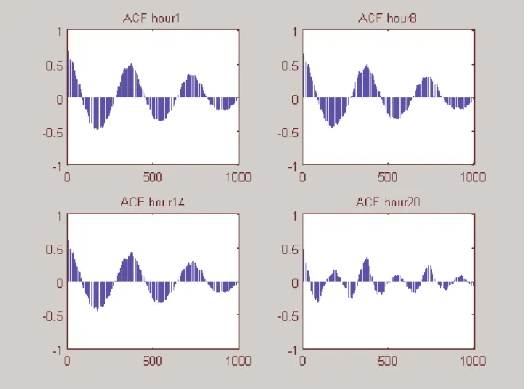
Figure 2 shows the autocorrelation function (ACF) of the series from December
26, 1990 to December 25, 1998 (eight years), for selected hours, after the trend and the
calendar effects (weekdays and holidays) are removed. The form of the ACF, which
resembles a damped sinusoid as in (5), with annual period, highly justifies using
Gegenbauer processes to model Zt. The exception is hour 20, in which either there is a
sinusoidal component of semiannual period or there are two sinusoidal components, one
with annual period and the other with semiannual period. This behavior does not occur
with any other hour, being specific of hour 20. However, our modeling does not add
another Gegenbauer factor (in the fashion of Ferrara and Guégan, 2000, 2001) to model
hour 20, obtaining good results though. In fact, hour 20 obtains the lowest errors, the
exception being one and sometimes two steps ahead, where it is beaten by hour 21.
2
We chose working with logarithms as the weekly seasonality and the holidays
effect can be modeled additively while they are multiplicative in the original series Xt.
These effects are believed to be multiplicative while relating to the average consuming
habits, varying proportionally when the number of consumers expands. This
demographic argument is justified by the Law of Large Numbers, since the aggregated
behavior is expected to reflect the average consumer behavior magnified by the sample
size (number of consumers). On the other hand, it ignores the effects that
macroeconomic forces may have on the load. Taking it into account, however, would
require a more complex modeling, not necessarily improving the accuracy of such a
short-term forecast horizon as the one considered in this paper. Other authors (e.g.,
Ramanathan, Granger and Engle, 1985) have also worked with load data in logarithms
to avoid heteroskedasticity, a similar argument to ours. However, we experimented
applying the same modeling as in (8)-(9) to Xt, instead of Yt, yielding very similar
results. Therefore, the choice of the logarithm transformation may be unnecessary for
such a short period (the four years estimation window plus one week of forecasts), but is
otherwise crucial if a much longer estimation window is used.
Soares and Souza (2003) have used the years 1995-1998 (four years) to estimate
the same model for the same series, having concluded that the degrees of fractional
integration, both seasonal and ordinary, vary throughout the hours, though d1 is always
positive (long memory) and d2 always negative (short memory). The (seasonal) long
memory is stronger for the hours in the beginning and in the end of the day, coinciding
with the hours where the load is smoother. The calendar effect, modeled by WDt and
αHt, is also not the same for all the hours, as it is apparent that days of the week and
holidays affect more the load in the middle hours (trading hours) than in the first or last
ones.
5 – Results
We run a forecasting exercise with the data specified in the previous section, evaluating
the results of model (8)-(9) when a structural break (the response to the energy-saving
campaign and the rationing scheme) is observed. The period used to evaluate the
forecasting performance includes from January 1, 2000 to September 30, 2002, and the
model is re-estimated each day. The forecast errors are evaluated one to seven days (24
to 168 hours) ahead, and for this we use the Mean Absolute Percentage Error (MAPE),
= + +
+ −
= n
i T i
i T i T X X X n MAPE 1 ˆ 1
, (10)
where Xt is the load at time t, Xˆ its estimate, T is the end of the in-sample and n is the t size of the out-of-sample. The MAPE measures the proportionality between error and
load, and is the most frequently used measure of forecasting accuracy in the load
forecasting literature (Darbellay and Slama, 2000, Park et al., 1991, Peng et al., 1992, to
cite but a few papers that use primarily this measure). Other measures could be used, as
some works suggest that these measures should penalize large errors and others suggest
that the measure should be easy to understand and related to the needs of the decision
makers. For an example of the former, Armstrong and Collopy (1992) suggest the Root
Mean Square Error (RMSE), while for an example of the latter, Bakirtzis et al. (1996)
use Mean Absolute Errors (MAE). However, these measures lack comparability if on
different data sets and for that reason the MAPE still remains as the standard measure in
the load forecasting literature. Some authors (c.f., Park et al., 1991, and Peng et al.,
1992) achieve MAPEs as low as 2% when predicting the total daily load, but results on
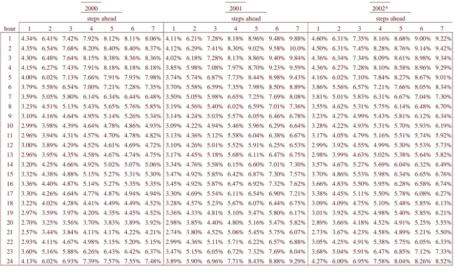
different data sets are not directly comparable as some are noisier than others. Table 1
shows the MAPEs for each hour, divided in three sets: the year of 2000 (before the
energy-saving campaign and the rationing scheme), the year of 2001 (more or less
during the campaign and the scheme), and from October 1, 2001 to September 30, 2002
(last year of data, part during the rationing period, part after the it was ended), which we
call 2002*. One could think of dividing the out-of-sample in periods before, during and
after the campaign, but they would not be directly comparable as there is seasonal
related heteroskedasticity in the data (forecast errors during the summer are in general
higher, as well as the load). This is due to the use of air conditioning appliances as cited
in Section 4.1. To compare different periods directly, they must comprise either an
integer multiple of one year or the same calendar periods in different years. We could
use a different division therefore, but decided to keep this one as it seems sufficient to
convey the most important features about the forecasting performance, before, during
and after the rationing period. It is clear from Table 1 that the forecasting performance
deteriorates a bit from 2000 to 2001, but not as much as one could expect provided there
is a structural break in the level of the load series. The results for one to three steps
ahead see even a reduction of the MAPE in the first and the last few hours (where the
remaining figures show in general an increase in the MAPE, of order of 0.2% on
average for one step ahead in the middle hours and increasing to around 2% for seven
steps ahead. From 2001 to 2002*, the one step ahead MAPEs increase in some hours
but for more than one step ahead the MAPEs always decrease. For example the
minimum and the maximum MAPEs one step ahead in 2000 are respectively 2.57%
(hour 21) and 4.35% (hour 2); in 2001, 2.74% (hour 21) and 4.12% (hour 2); and in
2002*, 2.73% (hour 21) and 4.60% (hour 1). For seven steps ahead the same figures are:
in 2000, 3.92% (hour 20) and 8.37% (hour 2); in 2001, 5.82% (hour 20) and 10.0%
(hour 2); and in 2002*, 5.50% (hour 21) and 9.42% (hour 2). It is important to note that
when we speak of h steps ahead, we consider the sectional data and hence refer to days.
As the primary data are hourly, one must interpret as 24h steps ahead, so that (1, 2, …,
7) daily steps ahead actually correspond to (7, 14, …, 168) hourly steps ahead.
Figure 3 shows one step ahead forecast errors for the period ranging from March
21, 2001 to September 7, 2001, for selected hours. Note that the errors become
consistently positive just the day after the possibility of electricity cut-offs was
announced (marked with a horizontal dashed line, in May 4, 125th day of 2001), showing that the forecasts become upward biased. The upward bias slowly decreases,
taking about a hundred days to level close to zero. The error range, on the other hand,
seems to decrease after this date for some hours. That is, although people knew about
the crisis at least in early March, and in April believed true a rationing scheme was
coming, this was not enough to change the aggregate consuming pattern. Only when
people became aware that their electricity supply could be compulsorily cut off, in early
May, they sensitized about the crisis and started saving energy. This was actually one
month before the rationing scheme was implemented.
Regarding the model, it is flexible enough to readapt its forecasts to the new
situation. During the smooth structural break, where the load level decreases slowly and
constantly, there is the slight bias commented in the above paragraph. After, when the
load seems to be located around a new level, it takes short to the forecasts become again
“apparently unbiased”. The forecasts themselves could be improved during and shortly
after the structural break, as a wise judgmental forecaster, knowing that an
energy-saving campaign was in course (and the rationing scheme about to be), could easily
improve forecasts by trying to gauge the observed bias. However, doing that in an
ex-post analysis like this one would be unfair, since by then people did not know what kind
leaving the forecasts as given by the model allows one to observe the public response to
new information.
Another distinct feature displayed by Figure 3 is the opposite effect, i.e. errors
consistently negative, before May 4. This feature ranges for approximately two weeks
and is possibly explained by the increase in the industrial activity observed, in order to
stock products for keeping up the sales during the coming rationing scheme.
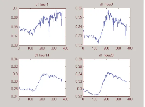
Figure 4 shows the evolution of the parameter d1 for selected hours, referring to
the intensity of the seasonal long memory, along the year 2001. In general this
parameter increases when the level downshift is in course, but afterwards, when this
downshift is already incorporated to the series, tends to revert towards its former range
of values. The exception is hour 1, representing the early and late hours when people are
expected to sleep, which seems to incorporate the change in d1. Note, however, that
even the changes observed in the estimated d1 for different hours are not considerable,
being noticed only because Figure 4 is small-scaled.
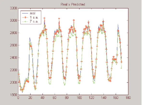
Figure 5 illustrates with a typical trading February week (not including Carnival
effects) the forecasting performance of the model (8)-(9). Both one and seven steps
ahead forecasts capture well the load profile, with the former being better than the latter
as expected. The week goes from February 4, 2001 to February 10, 2001 and is four
months before the rationing began. Note that there are two daily peaks, corresponding to
mid-afternoon (hottest time in the day) and the middle of the night (sleeping time). Air
conditioning appliances are responsible for this heavy load (it is worthwhile noticing
that February is summertime in the Southern hemisphere and that Brazil is mostly
situated in the tropical zone).
Figure 6 shows the forecasting performance of the model (8)-(9) just after the
consumption started decreasing, including from May 4, 2001 to May 17, 2001 (two
weeks, beginning on a Friday). This was the most critical period to forecast, as it is the
(supposed) beginning of the structural break. Note that the one step (24 hours) ahead
forecasts capture well the new dynamics, but the seven steps (168 hours) ahead
forecasts naturally fail to foresee the changes and as a result overestimate the load level,
taking longer to catch up on the new dynamics. However, approximately four months
after, the one and seven step ahead predictions get a very close fit to the load profile, as
can be seen in Figure 7. This figure shows the one step (24 hours) and seven steps (168
hours) ahead forecasts for the period from August 26, 2001 to September 1, 2001. Note
daily peak, as opposed to the two daily peaks observed in Figure 5 (corresponding to
February, at summertime). The variation in the load profile throughout the year was
previously mentioned in Section 1 as a motivation to use sectional data, but comparing
Figures 5 and 7 illustrates this feature. Note also that, additionally to the fact that Figure
7 illustrates a week during the rationing, there are much less load demanded from air
conditioning appliances in the winter, so that the load level displayed in Figure 7 is
considerably lower than that of February in Figure 5.
All the evidence leads us to conclude that even presenting a structural break,
some statistical properties of the electricity demand series are not lost, and these
properties are at least partially captured by the model proposed by Soares and Souza
(2003).
6 – Final remarks
This paper studies the forecasting performance of a stochastic model for the hourly
electricity load demand from the area covered by a specific Brazilian utility. The period
in study comprises an energy-saving campaign and a rationing scheme, which
constituted a structural break in the series level, lowering the average load demand by
about 20% if compared with the same period of the previous year. These almost
nationwide campaign and scheme were triggered by the 2001 Brazilian energetic crisis.
The crisis, in turn, was caused by a conjunction of events that occurred in Brazil, such
as an extremely dry period and lack of investments in generation and transmission,
allied to the fact that Brazil is energetically highly dependent on hydroelectricity.
The model used in this paper was proposed by Soares and Souza (2003) and
applies to sectional data, that is, the load for each hour of the day is treated separately as
a series. The model explains the seasonality by generalized (seasonal) long memory
using Gegenbauer processes, having in addition a stochastic level (driven by some
trend), and a calendar effects component (consisting of dummy variables for the days of
the week and for holidays).
Even in the presence of a structural break, the forecast accuracy does not suffer
dramatically, and the model rapidly readapts to the new situation. We conclude for the
presence of seasonal long memory in the data studied and that even the structural break
imposed by the rationing campaign was not able to destroy this statistical property. The
forecast errors from this model also allow one to observe the public response to
Acknowledgements
The authors would like to thank the Brazilian Center for Electricity Research (CEPEL)
for the data and Dominique Guégan for providing some bibliographical work. The first
author also would like to thank FAPERJ for the financial support.
References
Armstrong, J.S. and Collopy, F. (1992), “Error measures for generalizing about forecast
methods: empirical comparisons”, International Journal of Forecasting 8,
69-80.
Arteche, J. (2002), “Semiparametric robust tests on seasonal or cyclical long memory
time series”, Journal of Time Series Analysis 23, 251-285.
Baillie, R.T. (1996), “Long memory processes and fractional integration in
econometrics”, Journal of Econometrics 73, 5-59.
Bakirtzis, A.G., Petridis, V., Kiartzis, S.J., Alexiadis, M.C. and Maissis, A.H. (1996),
“A neural network short term load forecasting model for the Greek power
system”, IEEE Transactions on Power Systems 11, 858-863.
Beran, J. (1994). Statistics for Long Memory Processes (Chapman & Hall, London).
Bunn, D.W. and Farmer, E.D., Eds. (1985). Comparative Models for Electrical Load
Forecasting (John Wiley & Sons, Belfast).
Chung, C.-F. (1996), “Estimating a generalized long memory process”, Journal of
Econometrics 73, 237-259.
CNI, Confederação Nacional das Indústrias (2001a), “Efeitos do Racionamento de
Energia Elétrica na Indústria”, survey report, Jul 2001, 1-8.
CNI, Confederação Nacional das Indústrias (2001b), “Efeitos do racionamento de
energia elétrica”, Sondagem Industrial, suplemento especial Jul-Sep 2001, 1-2.
CNI, Confederação Nacional das Indústrias (2002), “Um ano após a crise energética”,
Sondagem Industrial, Ano 5, no. 2, 1-4.
Darbellay, G.A. and Slama, M. (2000), “Forecasting the short-term demand for
electricity. Do neural networks stand a better chance?”, International Journal of
Forecasting 16, 71-83.
Ferrara, L. and Guégan, D. (1999), “Estimation and applications of Gegenbauer
Ferrara, L. and Guégan, D. (2000), “Forecasting financial time series with generalized
long memory processes: theory and applications”, in C. Dunis (ed.), Advances in
Quantitative Asset Management, Kluwer Academic Press, 319-342.
Ferrara, L. and Guégan, D. (2001), “Forecasting with k-factor Gegenbauer processes:
theory and applications”, Journal of Forecasting 20, 581-601.
Fox, R. and Taqqu, M.S. (1986), “Large-sample properties of parameter estimates for
strongly dependent stationary Gaussian time series”, Annals of Statistics 14,
517-532.
Granger, C. W. G. and R. Joyeux (1980), “An introduction to long memory time series
models and fractional differencing”, Journal of Time Series Analysis 1, 15-29.
Gray, H.L., Zhang, N.-F. and Woodward, W.A. (1989), “On generalized fractional
processes”, Journal of Time Series Analysis 10, 233-257.
Hosking, J. (1981), “Fractional differencing”, Biometrika 68, 1, 165-176.
Hippert, H.S., Pedreira, C.E. and Souza R.C. (2001), “Neural networks for short-term
load forecasting: a review and evaluation”, IEEE Transactions on Power
Systems 16, 44-55.
Mandelbrot, B.B. (1977). Fractals: Form, Chance and Dimension (Freeman, San
Francisco).
Park, D.C., El-Sharkawi, M.A., Marks II, R.J., Atlas, L.E. and Damborg, M.J. (1991),
"Electric load forecasting using an artificial neural network", IEEE Transactions
on Power Systems 6 (2), 442-449.
Peng, T.M., Hubele, N.F. and Karady, G.G. (1992), “ Advancement in the application of
neural networks for short-term load forecasting”, IEEE Transactions on Power
Systems 7 (1), 250-256.
Porter-Hudak, S. (1990), “An application of the seasonal fractional differenced model to
the monetary aggregates”, Journal of the American Statistical Association 85,
338-344.
Ramanathan, R., Engle, R., Granger, C.W.J., Vahid-Araghi, F. and Brace, C. (1997),
“Short-run forecasts of electricity loads and peaks”, International Journal of
Forecasting 13, 161-174.
Ramanathan, R., Granger, C.W.J. and Engle, R. (1985), “Two-step modelling for
short-term forecasting”, in D. W. Bunn and E. D. Farmer (eds.), Comparative Models
Ray, B.K. (1993), “Long-range forecasting of IBM product revenues using a seasonal
fractionally differenced ARMA model”, International Journal of Forecasting 9,
255-269.
Soares, L.J. and Souza, L.R. (2003), “Forecasting electricity demand using generalized
long memory”, working paper, available at
http://www.fgv.br/epge/home/PisDownload/1160.pdf.
Soares, L.J. and Medeiros, M.C. (2003), “Modelling and Forecasting Short-term
Electricity Load: A Two Step Methodology”, working paper.
Table 1: MAPE for the years of 2000 (before rationing), 2001 (includes rationing in the end) and 2002* (includes rationing in the beginning). * from October 1, 2001 to September 30, 2002.
2000 2001 2002*
steps ahead steps ahead steps ahead
hour 1 2 3 4 5 6 7 1 2 3 4 5 6 7 1 2 3 4 5 6 7
Figure 5: Real versus predicted load (MWh), one and seven steps ahead, from February 4, 2001 to February 10, 2001 (one week, from Sunday to Saturday, approximately four months before the rationing began).