Fiscal Multipliers in Portugal Using a Threshold Approach

(1)

A Work Project, presented as part of the requirements for the Award of a Masters Degree in Economics from the NOVA – School of Business and Economics.

Fiscal Multipliers in Portugal Using a

Threshold Approach

Renato Poirier #557

A Project carried out on the Macroeconomics Major, under the supervision of:

Professor Luís Catela Nunes

(2)

Abstract

With Portugal in the midst of a huge economic crisis, many have proposed different solutions for the Portuguese problem. Being in the middle of an economic adjustment and after receiving assistance from external institutions, restoring the sustainability of national accounts has been the main priority. Fiscal consolidation has been made through cuts in public expenditure and higher government revenues. In this paper, using a TVAR framework, the effect of fiscal shocks in the real economy will be analyzed and fiscal multipliers will be estimated in periods of recession and expansion. Austerity measures that were taken by the Portuguese government will also be scrutinized and new possible scenarios will be added. The main finding of this paper is that Portugal should not only take measures regarding public deficit but must also implement measures that foster growth, especially through public expenditure.

Keywords:

 Fiscal Multipliers

 Expansion

 Recession

(3)

Content

1. Introduction ... 4

2. Literature Review ... 6

3. Methodology ... 8

3.1 The Model ... 8

3.2 Identification ... 11

4. Data ... 12

5. Results ... 14

5.1 Recession Period - 2009Q2 ... 14

5.2 Expansion Period – 1992Q1 ... 16

6. Actual Economy Measures Analyzed ... 17

7. Conclusion and Discussion ... 22

(4)

1. Introduction

With the Euro Area suffering a huge economic crisis, many European countries had to go through some tough economic plans, including austerity measures to maintain sustainable public accounts and adjust the level of public debt. One of those countries was Portugal. Portugal, plus Ireland and Greece needed assistance from the IMF and foreign institutions to have outside financing due to the high levels of sovereign debt yields, which required those countries pay huge amount of interest relative to previous years. In order for the IMF to lend assistance, Portugal had to commit himself to lower its budget deficit through higher taxes and government spending reductions so that, in a near future, the country could come back to external markets and get financing from private investors. So, national accounts consolidation became the number one priority for the Portuguese government. The path to achieve such consolidation was outlined by both the Portuguese government and the Troika1. It was decided by those entities that tough austerity measures had to be implemented to reduce the government budget deficit, through increases in both direct and indirect taxes and a decrease in government spending. Although the Portuguese society understood the need for a rapid adjustment, many economists and politicians appointed a huge flaw in this plan: no measures to foster growth and economic development. The decrease in government spending goes against the Keynesian theory, which defends that in times of economic distress, the role of government spending is highly important to boost the economy. Adding to that, we have the high level of distortion in the economy that is created by a high level of taxation, which gives incentives to lower consumption and decreases people’s confidence in the near future. The role of monetary policy in helping an economy to

1

(5)

recover is also important. But the main goal of this paper is to study the effect of fiscal policy. So knowing that real interest rates, which are manipulated by the ECB, have reached near the zero-bound point, its importance won’t be as high as the one played by fiscal policy.

It is very important to take into account the different economic situations that Portugal has passed through time and the different consequences that similar shocks have in different economic situations. For example, a shock of a certain magnitude in a period of recession will yield different outcomes, different effects on other economic variables, when comparing with shock of the same magnitude in an expansion period. In this research paper, one of the main goals will be to see how different are these outcomes, focusing on the output growth rate, when dealing with shocks on government spending and on net taxes in different economic situations. To answer those questions, a TVAR framework will be estimated and its results will be evaluated.

(6)

2. Literature Review

Suffering the effects of the financial crisis of 2008, the effect of fiscal policy on economic variables, more specifically on output, has been one of the most important research questions for economists. One of the benchmark papers, related to that subject, was the one made by Blanchard and Perroti (2002) (BP hereafter). The authors studied the dynamic effect of government spending and taxes on the U.S. output by using a structural VAR model (linear model). Their main finding was that positive government spending shocks had a positive effect on output, while the opposite happened when there were positive tax shocks. The output multiplier for government spending was estimated to be around one. A good summary of the literature made about fiscal multipliers until 2009, and all the methodology used until then, is the IMF report by Spilimbergo, Symansky and Schindler (2009). All results until that date, plus the theoretical concept of fiscal multipliers are presented. In the Portuguese case, government spending was estimated to be around 0.7 and the tax multiplier near 0. Pereira and Wemans (2013) used the same model as BP to evaluate the effect of fiscal shocks on output in the Portuguese economy. Their main findings were that an increase by 1€ in government spending would have a contemporaneous effect of 1€ on output and that in an one year span, the effect on output would be of around 30cent. Regarding taxes, the authors divided the effect of direct and indirect taxes, with the previous having a negative effect on output of 70cent in the next two years after the shock (1€) and the former followed the same sign as direct taxes, but the effects on output were smaller and not significant.

(7)

(8)

multipliers is magnified if the economy is in a recession, this is due to the fact that both multipliers are bigger in those regimes but the increase in the spending multiplier is more visible than in the tax multiplier (spending multiplier can be up to 10 times higher than the tax multiplier). Another very similar paper is the one by Baum, Poplowski-Ribeiro and Weter (2012), with the main difference being that they used both the output gap and the GDP growth as threshold in their estimation, and found no significant difference between the two methodologies. Similar results as in Batini et al. (2012) were obtained, plus adding the conclusion that fiscal policies must be tailored country-by-country depending on the macroeconomic situation of each country-by-country. Spending multipliers (8 quarters) went from 1.7 (USA) to 2.5 (Japan), German revenue multiplier was higher in periods of positive output gap. They also found that, spending shocks, when the output gap is negative, had a stronger effect when comparing with the same shock in an expansion period, being Canada the only exception. The main difference between the methodology used in the two last papers mentioned and the one by AG is that in the former, the threshold value was determined exogenously from the model while the first two the threshold was endogenous in the model. This difference will be explained later in the methodology section.

3. Methodology

3.1 The Model

(9)

capture the regimes switches and its critical value will be calculated endogenously. Many critical values for the threshold can be obtained, but in this specific paper, only one critical value will be used and it’s that value that will allow to separate the two regimes. The use of this model allows for a different evaluation on how fiscal multipliers behave in different economic situations. First of all, the fact that it is not a linear model like the standard VAR specification will allow to observe asymmetric reaction to shocks. Also because the effects of the shock depend on the size and sign of the shock plus on its initial conditions, we can differentiate between shocks in distinct regimes knowing that the impulse response functions are no longer linear. But most importantly, TVAR models can provoke regime switches (expansion to recession or vice-versa), due to the fact that the threshold variable of one of the endogenous variables. The TVAR model used in this research paper is similar to the one used in Baum and Koester (2011), and is the following:

(1) [ ]

Where is a three dimensional vector in which real output, government

spending and net taxes are included, [ ], the choice of this vector of variables was the same as the one used in BP (2002) and Baum and Koester (2011). The explanation from getting a TVAR from a standard VAR model is explained in

Appendix A. In this model, ( ); is a 3-dimensional vector that

contains deterministic terms (dummies, constant or even a time trend) and with ( depends on the number of states in the model, here we have only 2),

which are squared coefficient matrices of order 3. Secondly, ( ) .

(10)

covariance matrix of ∑ The threshold variable used in this model is represented by

, and it will determine in which regime we are working on. The function will take the value 1, when we are above the threshold critical value ( ) and 0 otherwise. It is also important to include at least one lag of the threshold variable so that it can be completely included in the TVAR model. Following previous literature (Batini et al. 2012), the value of will be set equal to 1. One of the main debates regarding this model is which threshold variable to use, the output gap or GDP growth? In this research paper, the threshold variable used was the output gap. This choice was made due to the fact that the output gap is more commonly used to identify economic cycles and is also considered a more reliable indicator for policy makers. Another important reason for the choice of the output gap over GDP growth, also mentioned by Baum et al. (2012), is the fact that fiscal policy has a bigger effect in the real economy in recessions than in expansions, when using the output gap as the threshold variable instead of the GDP growth2.

One important feature of using a TVAR framework instead of a linear VAR is the fact that the impulse response functions in a TVAR depend on the past history of the whole system until the time of the shock, while in a linear model this does not happen. What happens, when implementing a shock in a linear model, is that shocks are symmetric: opposite shocks with similar magnitude have the opposite effect but with the same magnitude, something that will not happen in a non-linear model. So what will be analyzed in this research paper are the generalized impulse response functions (GIRF), firstly studied by Koop et al. (1996). The GIRF’s will now allow for regime

2

(11)

switching (recession for expansion and vice-versa) after the implementation of a certain shock, depending on its size and if it is positive or negative3.

3.2Identification

The identification procedure will be the same as in Perroti and Blanchard (2002). In the TVAR model, we have to take into account the structural shocks between the

variables so that ̅ 4_{. So the vector of structural shocks in the model is given by}

_where _and _{represent the structural shocks}

for each variable. To better understand how these shocks are estimated, the following system is used:

(2) (3) (4)

In the first equation unexpected movements in taxes in a quarter can be explained by three different factors. The response due to unexpected movements in

GDP which are measured by , unexpected movements in government spending or a structural shock in taxes . The same line of thought is applied for the two

other equations. As in all the previous literature regarding this subject, three main steps are used to identify this system. The methodology regarding this part will follow the BP (2002) and Baum and Koester (2011) approaches. For the calculation of the parameters and , institutional information regarding tax and spending programs will be used.

3

In this model 1000 simulations were calculated, and the average value of those simulations was used for the impulse response function predictions.

4

(12)

Just like mentioned in BP, both automatic effects of economic activity of both variables depending on fiscal policy, and discretionary adjustments of fiscal policy can be explanations to unexpected movements in a quarter and will be taken into account. This last part will be nullified due to the fact that we are using quarterly data. So to have the values for both parameters, only the values of the elasticities to output of both taxes and government spending are needed, these elasticities were obtained from the work of André and Girouard (2005) (annual value). Regarding the elasticity of output to government spending, no automatic feedback was found or mentioned about, so the assumption that was taken. So after having the values for the first two parameters, and were estimated, by using the cyclically adjusted reduced-form tax

and spending residuals, and (knowing that ), afterwards we can use these estimates to find parameters and . One important feature on this model, and a huge topic for debate, is whether spending decisions come first ( ) or tax decisions come first ( ). The model was ran in both cases and results were very similar, so to follow a huge bulk of the previous literature, in this research paper, government spending decisions come first ( ).

4. Data

(13)

Banco de Portugal database. Regarding GDP, the values were taken from the OECD database (deflated by the GDP deflator where the value of 1 is taken in 2009 and were seasonally-adjusted). The output gap was calculated using the same methodology as in Baum and Koester (2011), by using the HP filter (λ=1600) in the real output series. So, the real output gap will be the difference between the actual real GDP and the real potential GDP divided by the real potential GDP. The unit roots tests5 were all made plus the lag length using the SIC criteria analysis was made. Afterwards, the logarithms of all variables were taken and then, first-differences were applied so that all variables became stationary, the only exception being the output gap variable which was already stationary at the beginning. The descriptive statistics, of all variables used in this research paper plus the graphs of all variables growth rates, are available in Appendix B. After analyzing the lag criteria and analyzing the previous literature, the TVAR model was run with one lag of each variable6.

After estimating the TVAR model, a threshold value of -0.0160558 was obtained. This is the value that minimizes the value of Squared Sum of Errors (Graph 1). Since this value is close to zero, it is possible to say that this model predicts two regimes: periods of positive output gap (expansion, above its potential) and negative periods (recession, below its potential). With this specification the model contains 89.77% of the observations above the threshold critical value and 10.33% of the observations below. The graph for the grid search for the threshold parameter results is presented in Appendix B.´

5

Augmented Dickey-Fuller Test and Phillips-Perron Test

6

(14)

5. Results

This section will be divided in two distinct parts. In the first, the analysis will be focused on shocks (1 and 2 standard deviations), in the revenue and spending variables, and its effect on output, both in periods of recession and expansion (which are determined by the output gap data obtained from the HP filter). In the second part, a more specific analysis will be made on the measures announced by the Portuguese government in the “Orçamento de Estado” in 2009 and 2010 and what were the effects of those measures on output. In this part, other possible scenarios will be presented, so that a comparison between the actual measures and those new scenarios is made. With this comparison, it will be possible to evaluate if the Portuguese government should have followed their austerity policy or followed another path. It has to be taken into account, that during the analysis of the results, some important economic factors are not taken into account like the national debt level, market confidence and expectations. Of course, if those variables were to be taken into account then probably the analysis of these results had to be different but that is not what we are looking for in this research paper. In the next part, positive and negative shocks of 1 and 2 standard deviations, on both government spending and net taxes, will be implemented in two distinct periods. Firstly, in 2009Q2, where we have a negative output gap, and then in 1992Q1, where we have a positive output gap. Then the measures of the Portuguese “Orçamento de Estado” from 2009 and 2010 will be analyzed and some other different scenarios will be evaluated.

5.1 Recession Period - 2009Q2

(15)

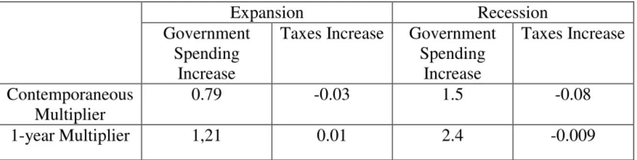
this part, the effect of positive and negative spending shocks is shown. In this period, having a positive shock in the government spending variable has a positive effect on output, which goes for the Keynesian theory (Graph 1). This conclusion can be taken by analyzing both the red and green line which are associated to a 1SD and 2SD, respectively. Comparing with the average output growth predicted by the model used, represented by the blue line, a positive shock in this variable would have increased output growth. The inverse happens when cutting government spending (negative shock), which are represented by the clear blue and black line, 1SD and 2SD, respectively. The model predicts that cutting government spending in times of recession would even depress more the economy and aggravate the decrease in output growth. As it is visible in the graph, the effects of such shocks would dissipate and return to the average predicted by the model in a period of 7/8 quarters. Contemporaneous multipliers relative to positive shocks were found to be around 1.5 and 1-year cumulative multiplier of 2.4 for a positive shock in government spending.

Graph 1 – Government Spending Shocks (Positive and Negative) effect on Output (2009Q2)

Relative to tax shocks (Graph 2), the verified effect on output growth was the inverse, when comparing with the spending shocks presented in the former paragraph. A positive tax shock of 1SD would decrease output growth and the negative effect is even bigger when applying a 2SD shock (clear blue line). The inverse happens when we

Green Line – Positive Shock 2SD

Red Line – Positive Shock 1SD

Clear Blue Line – Negative Shock 1SD

Black Line – Negative Shock 2SD

(16)

have a tax cut in that period. Similarly to what happened with spending shocks, tax shocks tend to dissipate in 6/7 quarters. The cumulative tax multiplier for the portuguese economy is around 0.08 and 1year cummulative multiplier were around -0.009 relative to a tax hike.

Graph 2 – Tax Shocks (Positive and Negative) effect on Output (2009Q2)

5.2Expansion Period – 1992Q1

The fact that in this period, the Portuguese economy was facing a huge growth was due to the fact that Portugal had entered in the European Union in 1986 and was still receiving European funds, and those were used to invest in new infrastructures and in some important areas like education or health, so that Portugal could catch up with the other members of the EU. As in recession periods, a positive shock in government spending would have had a positive effect in output, increasing its growth rate, but for a shock of both 1SD and 2SD (red and green line respectively), the magnitude of the shock will be lower than in the recession case (Graph 3). Contemporaneous Multiplier of 0.79 and the value of a 1-year cumulative multiplier of 1.21 were estimated for the Portuguese economy. From the analysis of these values, comparing with those found in a recession period, one important conclusion can be already derived: government spending multipliers in periods of recession are higher than those found in periods of

Green Line – Positive Shock 2SD (Tax Hike)

(17)

expansion, meaning that a policy focused on higher spending can have important effects in taking an economy from its recessive period.

Regarding shocks in taxes, the same will happens as in the recession periods but once again the magnitude of the shock will be lower but not to the extent as what happened for government spending. Contemporaneous multiplier of around -0.03 and 1-year cumulative multiplier of 0.01 were found for Portugal.

6. Actual Economy Measures Analyzed

Not only is important for people to know how the real economy behaves in good and bad times after implementing shocks in some macroeconomic variables, but it is also important to analyze political decisions. As mentioned in the introduction, Portugal

Blue Line – Average Output Growth

(18)

is facing a debt crisis and austerity measures have been implemented in order to balance national accounts and gain market confidence once again. One of the main debates in the Portuguese society is whether Portugal should continue with the austerity measures implemented by the government, or if a policy that also focus on economic growth should be put into plan. So after the analysis of how output behaved in times of recession and expansion after implementing shocks in two important macroeconomic variables, in this section it will be seen how output growth behaved when implementing the measures written in the “Orçamento de Estado” of 2009 and 2010. Not only we will see the effect of those measures but also some other scenarios will be estimated, in order to see if the path followed by the Portuguese government has been the right one or a change in policy should have been made.

(19)

Graph 5 – Implementing a shock of G=-1.5% and T=2.7% (2008Q3)

From the former graph, it is possible to see that with the implementation of the previous announced measures, on the two last quarters of 2008, output growth decreased when comparing with the predicted average output growth. But the real difference is when we look at the first quarter of 2009, where the model predicts a huge fall in the output growth (from 1.3% to almost -0.4%). With the implementation of these measures, the fall will be somewhat accommodated (approximately -0.15%), but quickly will reach the values that were initially predicted in the model. Although in the next periods, the output growth rate with the implemented shock would be the same as the rate predicted initially by the model (even though the new output growth rate is slightly higher than the one predicted but not significant).

In order to compare, a scenario where the increase in government revenue will be of 2% and a government spending increase of 2% (once again, Portugal probably would not be able to implement such a policy due to budget targets and exterior pressure but still it is important to analyze all scenarios). So Graph 6 presents the simulation of this scenario. Comparing with the real scenario, we can see that in the short-run, output growth rate would stay very similar to the one predicted in the model and that this measure would also accommodate the huge fall in the output growth rate, even though not as much as in the previous graph. The main difference between the two

Red Line – Output Growth with G=-1.5% and T=2.7%

(20)

graphs is the fact that with this new scenario the output growth rate would be above the one predicted by the model and increasing the difference around the first/second quarter of 2010.

Graph 6 – Implementing a shock of G=2% and T=2% (2008Q3)

Even though in the first simulation, the huge fall in the output growth rate was more accommodated than in the first, probably it can be explained due to external factors to the model (maybe, foreign investors and other countries perceived these measures as a positive sign of commitment by the Portuguese government which allowed output to not decline as much). With the second simulation, it is possible to see that although increasing revenue, a higher output growth rate would be possible if it was accompanied by an increase in government spending, which is a result consistent with what was previously said about the effect of government spending multipliers in the Portuguese economy.

As said previously, the same methodology for the measures announced in the “Orçamento de Estado” of 2010 will be used. In that report, the Portuguese government announced that their main goal was to reduce public expenditure by 0.2% and still increase tax revenues by 1.2% relatively to the previous year. Just like in the OE2009, the measures announced will be put in the model in the third quarter of 2009.

Red Line – Output Growth with G=2% and T=2%

(21)

Graph 7 – Implementing a shock of G=-0.2% and T=1.2% (2009Q3)

By observing the previous graph, it is possible to observe that up until 2010Q3, the output growth rate induced by these measures was higher than the one predicted by the TVAR model, which would be a positive point for the Portuguese economy. But the problem with these measures would be afterwards, where output growth would decrease to even lower levels than those predicted by the model if no shocks were implemented. Such downfall can be explained by the fact, that people and firms interpreted such measures as temporary and expected that higher taxes would be compensated by either a decrease in the future tax rate or higher government spending, something that did not happen in reality, with the Portuguese government continuing with the austerity measures, which would put the Portuguese economy worse off. So due to this interpretation, let’s build a scenario where the government decides to keep the growth of public spending at the same rate as before, G=0%, and raise tax revenues by 3%, T=3%. The analysis of such scenario can be made through Graph 8.

– Implementing a shock of G=0% and T=3% (2009Q3)

Red Line – Output Growth with G=-0.2% and T=1.2%

Blue Line – Average Output Growth with no Shock

Red Line – Output Growth with G=0% and T=3%

(22)

As it is possible to observe, increase tax revenues by 3% will not make output increase at a lower rate than in the previous scenario, but it will have more recessive effects in 2011, where the growth rate of output will decrease even more than before. Also the fact that the Portuguese government does not decrease government spending in a drastic way does not counteract against the negative effect of higher taxes.

7. Conclusion and Discussion

Table 1 – Fiscal Multiplier Results Summary

Expansion Recession

Government Spending

Increase

Taxes Increase Government Spending

Increase

Taxes Increase

Contemporaneous Multiplier

0.79 -0.03 1.5 -0.08

1-year Multiplier 1,21 0.01 2.4 -0.009

(23)

(24)

8. References

Afonso, A., J. Baxa and M. Slavik, 2011, “Fiscal Developments and Financial Stress: A Threshold VAR Analysis”, ECB Working Paper No. 1319

Auerbach, A.J., and Y. Gorodnichenko, 2012a, “Measuring the Output Responses to Fiscal Policy,” American Economic Journal: Economic Policy, Vol.4, pp. 1-27

Auerbach, A.J., and Y. Gorodnichenko, 2012b, “Fiscal Multipliers in Recession and Expansion,” in “Fiscal Policy after the Financial Crisis,” A. Alesina and F. Giavazzi, (eds.), University of Chicago Press

Batini, N., G. Callegari, and G. Melina, 2012, “Successful Austerity in the United States, Europe and Japan”, IMF Working Paper 12/190

Baum, A. and G.B. Koester, 2011, “The Impact of Fiscal Policy on Economic Activity over the Business Cycle – Evidence from a Threshold VAR Analysis,” Bundesbank Discussion Paper, 03/2011

Baum, A., Poplawski-Ribeiro, M., and A. Weber, 2012, “Fiscal Multipliers and the State of the Economy” IMF Working Paper 12/286

Blanchard, O., and R. Perroti, 2002, “An Empirical Characterization of the Dynamic Effects of Changes in Government Spending and Taxes on Output,” Quarterly Journal of Economics, Vol. 117, pp. 1329-1368

(25)

Koop, G., Pesaran, M. H. and S. M. Potter, 1996, “Impulse Response Analysis in Nonlinear Multivariate Models”, Journal of Econometrics 74(1), pp. 119-147

Pereira, M., and L. Wemans, 2013, “Output Effect of Fiscal Policy in Portugal: a Structural VAR Approach”, Economic Bulletin, Spring 2013, Banco de Portugal

Spilimbergo, A., Symansky, S., and M. Schindler, 2009, “Fiscal Multipliers” IMF Staff Position Note, SPN/09/11, May 2009

(26)

A Work Project, presented as part of the requirements for the Award of a Masters Degree in Economics from the NOVA – School of Business and Economics.

Fiscal Multipliers in Portugal Using a

Threshold Approach (Appendix)

Renato Poirier #557

A Project carried out on the Macroeconomics Major, under the supervision of:

Professor Luís Catela Nunes

(27)

Appendix A

The methodology presented in this Appendix was the same as used in Baum and Koester (2011). We have a standard VAR with stationary endogenous variables, with

and of finite order :

(1)

Where is a -dimensional vector (is this research paper ), and it contains a constant, a linear time trend or even if necessary some dummy variables (which is not the case for this specific research paper). is a 3 dimensional squared coefficient matrix where (in this research paper ) and are the uncorrelated random errors with zero mean and a covariance matrix of ∑ It is possible to rewrite equation (1) as:

(2)

Where ( ) and . So now it is possible to

obtain the TVAR model presented in the methodology section.

(28)

Appendix B

 Variables Growth Rates1

Graph 1 – Output Growth Rate Graph 2 – Government Spending Growth Rate

Graph 3 – Taxes Growth Rate Graph 4 – Output Gap

1_{After analyzing the unit root tests and apply first-differences on all variable, except the output gap which}

(29)

Table 1 – Descriptive Statistics of the Variables

Mean Max Min Standard Deviation

Government Spending

0.016029 0.045765 -0.508362 0.209509

Taxes 0.014023 0.511068 -0.469627 0.171802 GDP 0.011577 0.054038 -0.022863 0.012801 Output Gap 8.75e-13 0.029012 -0.051482 0.014353

(30)

Appendix C

 2006Q4 (Output Gap=0)

Blue Line – Average Output Growth