Annales Geophysicae, 23, 827–830, 2005 SRef-ID: 1432-0576/ag/2005-23-827 © European Geosciences Union 2005
Annales
Geophysicae
The ionospheric heating beneath the magnetospheric cleft revisited
G. W. Pr¨olss
Institut f¨ur Astrophysik und Extraterrestrische Forschung, Universit¨at Bonn, Auf dem H¨ugel 71, 53121 Bonn, Germany Received: 10 September 2004 – Revised: 9 December 2004 – Accepted: 15 December 2004 – Published: 30 March 2005
Abstract. A prominent peak in the electron temperature of the topside ionosphere is observed beneath the magne-tospheric cleft. The present study uses DE-2 data obtained in the Northern Winter Hemisphere to investigate this phe-nomenon. First, the dependence of the location and magni-tude of the temperature peak on the magnetic activity is de-termined. Next, using a superposed epoch analysis, the mean latitudinal profile of the temperature enhancement is derived. The results of the present study are compared primarily with those obtained by Titheridge (1976), but also with more re-cent observations and theoretical predictions.
Keywords. Ionosphere (Polar ionosphere; Plasma tempera-ture and density) – Magnetospheric physics (Magnetosphere-ionosphere interactions)
1 Introduction
One of the most striking features of the dayside polar iono-sphere is the sudden increase in the electron temperature be-neath the magnetospheric cleft. The first to study this heat-ing effect was Titheridge (1976). Usheat-ing data derived from Alouette-1 top side ionograms, he presented mean latitu-dinal profiles of the temperature enhancement and investi-gated their dependence on magnetic activity and interplan-etary conditions. Evidently, the scientific community was so impressed by this study that it did not take up the sub-ject again and/or discontinued work in the field. As a con-sequence both the effect itself and especially the paper by Titheridge almost fell into oblivion. This prompted the au-thor to repeat the study of Titheridge, however, this time us-ing DE-2 data with their greatly improved spatial resolution. This higher resolution also allowed for more refined analyz-ing methods, and these are described in the followanalyz-ing sec-tions.
2 Data selection and processing
A general description of the DE-2 satellite was given by Hoffman and Schmerling (1981), and details on the Correspondence to:G. W. Pr¨olss
Langmuir probe experiment can be found in Krehbiel et al. (1981). First electron temperature and density measure-ments obtained by this instrument were discussed in Brace et al. (1982).
In order to extract the cleft effect on the electron tempera-ture from the unified abstract file of the DE-2 data set, all or-bits were divided into four segments, each of which extended from equatorial to polar latitudes. Of these data segments only those obtained in the Northern Hemisphere within±45 days of the December solstice and within the 09:00–15:00 h magnetic local time sector were retained. This is because in the Titheridge study most of the data refer to the same conditions. The selection procedure resulted in a total of 188 orbital segments with sufficient data coverage. For each of these segments, the electron temperature was plotted as a function of invariant latitude and displayed on a terminal screen. As it turned out, clear cleft signatures were observed in nearly all of these temperature profiles, testifying to the quasi-permanent presence of this feature. The terminal plots were also used to roughly parameterize the heating effect. Thus, the latitudes of the equatorward boundary and the max-imum of the temperature enhancement, together with their respective temperature values, were determined; see Fig. 1. Since the poleward boundary was often poorly defined, this was not considered. Altogether, 179 temperature profiles and their associated parameter sets are analyzed in the following study.
3 Location and magnitude of the temperature enhance-ment as functions of magnetic activity
828 G. W. Pr¨olss: The ionospheric heating beneath the magnetospheric cleft revisited
Fig. 1.Example of an electron temperature enhancement in the day-side polar region. Shown are data obtained by the DE-2 satellite on 18 January 1983 in the Northern Hemisphere. The measurements refer to a magnetic local time of approximately 13:10 h and to mod-erate magnetic activity. The observation heights are indicated in the upper part of the figure. Vertical lines mark the equatorward bound-ary and the maximum of the temperature increase.
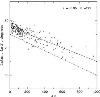
Fig. 2. Changes in the position of the temperature peak with the level of magnetic activity. The scatter plot shows the invariant lat-itude of the maximum of the temperature enhancementLat mas a function of the hourly averagedAEindex. A straight line has been fitted to the data: Lat m[deg]=77.8−0.013·AE (solid line). The regression coefficient reaches 0.85 and the total number of data points is 179. Also shown is the regression line for the invariant latitude of the equatorward boundary of the temperature increase: Latf[deg]=75.0−0.015·AE(dashed line).
latitudes (dashed line). Extrapolating both lines toAE=0, we find that during magnetically quiet conditions the equa-torward boundary and the temperature maximum should be located at about 75◦and 78◦invariant latitude, respectively.
The latitude of the temperature maximum was also corre-lated with other magnetic activity indices like theKp,apand
Dst indices, partly including the temporal development of
these indices. As it worked out, these correlations were not as good as for theAEindex. A similarly high correlation
coeffi-Fig. 3. Changes in the magnitude of the temperature peak with the level of magnetic activity. Shown is a scatter plot of the maxi-mum temperaturesT emas a function of the hourly averagedAE index. These temperatures have been adjusted to a common al-titude of 600 km. Also shown is the respective regression line: T em[K]=2712+2.4·AE.
cient was obtained only for the negativeBzcomponent of the
interplanetary magnetic field. We also checked Titheridge’s suggestion that the location of the temperature enhancement depends on the sector polarity of the interplanetary magnetic field. No correlation of this kind was observed.
Finally, the dependence of the magnitude of the temper-ature increase on the level of magnetic activity was investi-gated. To this end the peak temperature was plotted as a func-tion of theAEindex; see Fig. 3. As can be seen, the scatter of the data points is quite large and the correlation coefficient correspondingly low (r=0.55). There is, however, a general trend for the heating effects to become larger with increas-ing magnetic activity. A somewhat better correlation was obtained when theAE index was replaced by the dynamic pressure of the solar wind or the product of these quantities.
4 Mean latitudinal profile
As illustrated in Fig. 1, the temperature enhancement in the cleft region is confined to a relatively narrow latitudinal range. Also, its position is constantly changing in response to changes in geomagnetic activity. Therefore, special care must be exercised when deriving the mean latitudinal pro-file of this phenomenon. Here the following procedure was adopted.
G. W. Pr¨olss: The ionospheric heating beneath the magnetospheric cleft revisited 829 analysis was performed to estimate the temperature
gradi-ent in the topside ionosphere. For the data set at hand, this ranged between about 2 and 3 K/km. To simplify matters, a constant temperature gradient of 2.5 K/km was used for the height adjustment.
In a second step all available latitudinal profiles (includ-ing that shown in Fig. 1) were superimposed in such a way that the maxima of the temperature enhancements were aligned and located at a common reference latitude (super-posed epoch analysis). This way the basic latitudinal struc-ture of the temperastruc-ture enhancement was kept intact and not smeared out by the averaging procedure.
In a third step the median and the upper and lower quartiles of the temperature values were determined for each latitude. Finally, spline curves were fitted to these parameters. The end product of this procedure is shown in Fig. 4. Here the latitude coordinates refer to anAEindex of 200. This axis should be shifted to the left or right depending on the respec-tive level of magnetic activity.
As is evident from Fig. 4, the mean electron temperature enhancement in the cleft region stands out as an isolated narrow peak similar to that shown in Fig. 1. The tempera-ture increase is of the order of 1200 K, which corresponds to a relative increase of about 60%. At the same time, the full width of the temperature enhancement is about 6◦. These properties should be compared with those derived by Titheridge (op. cit.), whose mean latitudinal profile is also shown (dashed line; note that this profile was obtained by in-terpolating his profiles for 400 and 1000 km altitude). As is evident, the mean temperature increase derived by this author is considerably smaller and much wider. This is not surpris-ing considersurpris-ing the relatively crude latitudinal resolution of the data set at his disposal and the averaging procedure em-ployed.
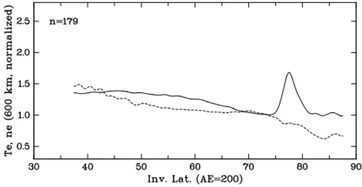
How does the electron density behave in the neighborhood of the temperature peak? To answer this question, mean lati-tudinal profiles of the electron density were generated, again using the latitude of the peak electron temperature as a com-mon reference location. We find that on the average a slight decrease in the electron density is observed near the temper-ature enhancement; see Fig. 5. If individual profiles are ex-amined, both increases and trough-like decreases in the elec-tron density are observed, but most of the time these are not strictly co-located with the temperature enhancement.
5 Discussion
The present study provides an improved description of the ionospheric heating effect beneath the magnetospheric cleft. This should prove useful in several respects.
First, such a description may be incorporated into empir-ical models of the ionosphere. The International Reference Ionosphere, for example, does not contain a specification of this phenomenon (Bilitza, 2001).
Second, the derived heating effect should be compared with the results of theoretical studies. Take, for example,
Fig. 4.Mean latitudinal profile of the electron temperature enhance-ment in the dayside polar region in winter. Plotted is the median of 179 temperature profiles which have been superimposed in such a way that the latitude of the temperature peak serves as a com-mon reference location. The shaded area indicates the range be-tween the lower and upper quartiles. The specific latitudes indi-cated on the abscissa apply for an hourly averagedAEindex of 200 (see Fig. 2). Also shown is the mean latitudinal profile derived by Titheridge (1976) for similar conditions (dashed line). All temper-atures refer to a common altitude of 600 km.
Fig. 5.Comparison of the mean latitudinal profiles of electron tem-perature (solid line) and electron density (dashed line) in the dayside polar region in winter. The format of data presentation is similiar to that used in Fig. 4, except that in addition to the height adjustment, the data have also been normalized. Here the temperature and den-sity recorded at the equatorward boundary of the temperature peak (i.e. atLatf) served as reference values.
the recent simulation study by Vontrat-Reberac et al. (2001). These authors find that immediately after turning on the cusp precipitation in their ionospheric model, the electron temper-ature in the topside ionosphere increases by about 1000 K, which is close to what is actually observed on the average. Also, the lack of a clear signature of the cleft precipitation on the electron density seems to be understood (e.g. Pitout and Blelly, 2003).
830 G. W. Pr¨olss: The ionospheric heating beneath the magnetospheric cleft revisited particle precipitation in the cleft region (e.g. Carbary and
Meng, 1986). The latter study, for example, specifies the equatorward shift of the cleft precipitation with increasing magnetic activity. They find that for moderate magnetic ac-tivity (AE(1 min)=200), the center of the precipitation region is located near 76◦, which is close to where the temperature peak is observed in the present study for similar conditions.
Finally, the close connection between ionospheric and thermospheric heating effects should be pointed out. Whereas the lower thermosphere beneath the cleft region is primarily heated by ionospheric currents (e.g. Pr¨olss, 1981; L¨uhr et al., 2004), the upper thermosphere is also heated by the hot electron gas. This thermal coupling deserves further study.
A more detailed comparison with theory and other obser-vations has been postponed until a larger data set is available. This extended data set will include measurements obtained during all seasons and in both hemispheres.
Acknowledgements. The DE-2 data used in this study were kindly provided by the NASA National Space Science Data Center. I am grateful to all the experimenters who contributed to this data set. I am also indebted to Ben Bekhti, N., Schr¨ufer, K., and Winkel, B. for their help in preparing this manuscript.
Topical Editor T. Pulkkinen thanks J. E. Titheridge for his help in evaluating this paper.
References
Bilitza, D.: International Reference Ionosphere 2000, Radio Sci., 36, 261–275, 2001.
Brace, L. H., Theis, R. F., and Hoegy, W. R.: A global view of F-region electron density and temperature at solar maximum, Geo-phys. Res. Lett., 9, 989–992, 1982.
Carbary, J. F. and Meng, C. I.: Correlation of cusp latitude withBz andAE(12) using nearly one year’s data, J. Geophys. Res., 91, 10 047–10 054, 1986.
Doe, R. A., Kelly, J. D., and S´anchez, E. R.: Observations of persis-tent dayside F region electron temperature enhancements associ-ated with soft magnetosheathlike precipitation, J. Geophys. Res., 106, 3615–3630, 2001.
Hoffman, R. A. and Schmerling, E. R.: Dynamics Explorer pro-gram: An overview, Spaces Sci. Instr., 5, 345–348, 1981. Krehbiel, J. P., Brace, L. H., Theis, R. F., Pinkus, W. H., and
Ka-plan, R. B.: The Dynamics Explorer Langmuir probe instrument, Space Sci. Instr., 5, 493–502, 1981.
L¨uhr, H., Rother, M., K¨ohler, W., Ritter, P., and Grunwaldt, L.: Thermospheric up-welling in the cusp region, evidence from CHAMP observations, Geophys. Res. Lett., 31(L06905), doi:10.1029/2003GL019314, 2004.
Pitout, F. and Blelly, P.-L.: Electron density in the cusp iono-sphere: increase or depletion?, Geophys. Res. Lett., 30(14), doi:10.1029/2003GL017151, 2003.
Pr¨olss, G. W.: Latitudinal structure and extension of the polar at-mospheric disturbance, J. Geophys. Res., 86, 2385–2396, 1981. Sandholt, P. E., Carlson, H. C., and Egeland, A.: Dayside and polar
cap aurora, Kluwer Acad. Publ., Dordrecht, 2002.
Titheridge, J. E.: Ionospheric heating beneath the magnetospheric cleft, J. Geophys. Res., 81, 3221–3226, 1976.