Abstract— In this paper, a simple and accurate technique for the
measurement of the S-Parameters of a two-port network from time domain data is presented, based on Fourier theory and techniques. This method is proposed to circumvent the need of a network analyser when studying an unknown device, as no additional measurements other than the time domain data are required. An excellent correspondence between this technique's results and regular network analyser measurements is achieved for the entire operational band of the devices tested.
Index Terms—Instrumentation, Microwave, Signal Processing, Time Domain
Reflection.
I.INTRODUCTION
In the microwave community, scattering parameters (S-parameters) are frequently used to
characterize a device under test (DUT). It has been shown that power waves and the corresponding
scattering matrix give a clear understanding of the power relations between circuit elements connected
through a multiport network [1]. Microwave measurement techniques for component and system
characterization and modeling can be categorized as Frequency Domain Measurements Techniques
(FDMT) and Time Domain Measurements Techniques (TDMT) [2]. In this paper, the focus will be in
extracting frequency information from a time domain method. In this technique, a network can be
analyzed in two ways: the Time Domain Reflection (TDR) and the Time Domain Transmission
(TDT) methods. Due to the lower costs of TDR and TDT instruments, the acquisition of
domain parameters by using time-domain data is a growing alternative to traditional
frequency-domain analysis [3].
In this paper it is described a method of extracting the S-parameters of a device under test by the
use of TDR and TDT techniques. The Discrete Fourier Transform is applied to the incident and the
reflected/transmitted signals. The reflection/transmission coefficients are obtained by the division of
the transformed reflected/transmitted signals to the transformed incident signal. All the processing is
done by the use of the software MATLAB.
II. TIME DOMAIN MEASUREMENTS IN MICROWAVE FREQUENCIES
Signal Processing Technique for Time Domain
Measurement of S-Parameters
Isabela M. Nobre, Julio L. Nicolini, Joaquim D. Garcia, Marbey Mosso
Centre of Studies in Telecomunications, Department of Electrical Engineering, Pontifical Catholic University of Rio de Janeiro, Rio de Janeiro, Brazil
The step is launched into the transmission line under test. The oscilloscope monitors the incident and
reflected voltage at a particular point of the line. In the display, it is possible to have information
about the impedance of the line, along with the position and nature of each discontinuity [4].
Noise is an important factor in data analysis in laboratory measurements. All laboratory procedures
are subject to a variety of noise sources, therefore a processing technique is used in the results of TDR
and TDT measurements realized in this work to minimize noise. Many filters can be used to smooth
the time domain measurements, such as the l1 trend filter [5], the Savintsky Golay filter [6] and the
Hodrick Prescott filter [7]. The Hodrick Prescott filter was initially used on econometrics, however as
it has smoother results it has also found applications in chemistry [8] and control theory [9]. In this
paper we use the Hodrick Prescott filter to smooth and remove part of the noise of the time domain
signal.
III. MATHEMATICAL MODEL
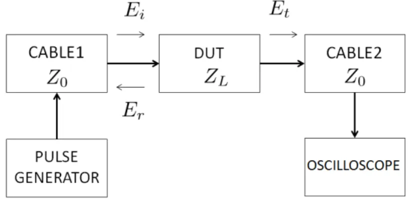
A. Electromagnetic Theory
If the load connected to the cable has different impedance, as shown in figure 1, Maxwell's
equations are only satisfied if a second wave is originated at the load and propagates back towards the
source. The ratio of the reflected wave to the incident wave is defined as the reflection coefficient
[10]:
(1)
If a mismatch exists at the load, the reflected wave will be added algebraically to the incident wave
at the oscilloscope display [4]. Since it is separated in time from the incident wave, the reflected wave
can be identified. The shape is also valuable to reveal the nature and the magnitude of the mismatch.
The same is valid for the transmitted wave, which exists to ensure Maxwell's equations on the other
side of the discontinuity. The transmission coefficient can be defined as [10]:
(2)
By this method, it is obtained the responses in time to the step generator (transmitted and
Fig. 1. Circuit block diagram.
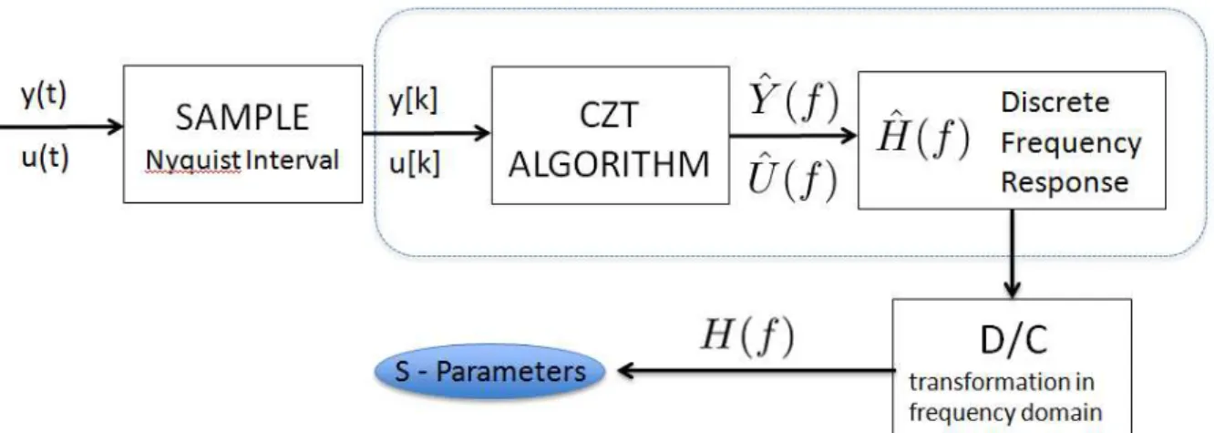
B. Data Processing
To extract the continuous signals for future computer analysis, it is required to perform a sampling.
A continuous signal sampled on a grid finer than the Nyquist interval can be, in principle, perfectly
reconstructed via interpolation, since the sampling does not compromise the information content of
the signal.
The Nyquist interval is the upper bound on the sampling interval of a discretized signal in the time
domain such that the sample contains all the available frequency information of the signal.
The Nyquist–Shannon sampling theorem states [11]:
“If a function x(t) contains no frequencies higher than B Hertz, it is completely determined by giving its ordinates at a series of points spaced 1/2B seconds apart”
The threshold 2B is called the Nyquist rate and 1/2B is the Nyquist interval.
By the use of the proper sampling rate, we obtain the output and input signals in the discrete time
domain. They are related to the discrete time impulse response by the following:
(3)
Where y[k] is the sampled output signal, u[k] the sampled input signal, h[k] the discrete- time
impulse response, and the “*” signal denotes the convolution sum operation [12], given by:
(4)
The discrete-time impulse response is related to the scattering parameters. It is also more directly
related to the discrete transfer function of the system through the use of the Discrete Fourier
Transform (DFT). The DFT of a signal x[k] can be defined as [13]:
(5)
(7)
The transformation to the frequency domain of y[k] and u[k] is done by the Chirp Z-Transform
algorithm (CZT). The reference [14] discusses this algorithm in details. In this reference, it is stated
that the CZT is
``A computational algorithm for numerically evaluating the z-transform of a sequence of N samples.''
The z-transform is defined as
(8)
And its computation is facilitated by the CZT algorithm. The DFT is a special case of the
z-transform and it has some limitations which can be eliminated using the CZT algorithm [14].
The reference [15] shows that the relationship between a continuous frequency response H and its corresponding discrete frequency response Ĥ is:
(9)
Where Π is a rectangle function, Δ is a sampling function, T is the sample period and K is defined
as the integer impulse response sample length. This reference also explores issues with real time
domain responses, time aliasing, causality, interpolation and re-sampling of discrete frequency data,
which are useful to perform the signal processing properly.
Finally, with the H function, the S-parameters can be obtained. If the analysis was made to the
reflected signal (TDR), the scattering parameters S11(source in port 1) and S22 (source in port 2) can
be achieved. S11 in dB is given by:
(10)
However, if the analysis is made to the transmitted signal (TDT), the scattering parameters S21
(source in port 1) and S12 (source in port 2) can be achieved. S21 in dB is given by:
Fig. 2-(a). Block diagram of the signal processing steps.
Fig. 2-(b). Alternate implementation of the dashed blue area.
Figure 2-(a) shows a block diagram representation of the signal processing that has been discussed,
while figure 2-(b) shows an alternative implementation for the dashed blue area; note that this
alternative is only possible if the input signal is a step function, due to the linearity of the
differentiation operator. This alternative implementation is simpler, as there is no requirement for
the input signal to be measured, stored and processed, lowering computational costs.
C. Filtering Noisy Data
Let denote the discrete signal obtained either from TDR or TDT as y, thus yk represents the k th
position of vector y. Since we are supposing that the data is noisy, y is a sum of the theoretical signal w and a error ϵ that we assume Gaussian [16]. In other words y = w + ϵ. The Hodrick Prescott filter is defined as follows:
(12)
The first sum minimizes the error, which means that the output of the filter must keep similarity
with the noisy signal. The second sum is used for minimizing the second difference of the output
signal, thus minimizing the variation of the signal's derivative. For the second sum, λ is a parameter
that controls how fine the smoothing will be. The resulting signal is a smoother approximation of the
original noisy data.
IV. EXPERIMENTAL RESULTS
Using a pulse generator, a step signal is generated. Before the device under test (DUT) can be
Fig. 3-(a). Block diagram of the experimental setup.
Fig. 3-(b). Experimental setup.
The time domain response data from the coaxial cable can be saved for later processing, and the
DUT is added to the network. As discussed in the previous section, the step signal will create reflected
and transmitted pulses upon interacting with the DUT, and both of those pulses are recorded by the
time domain oscilloscope, with their data saved to a computer.
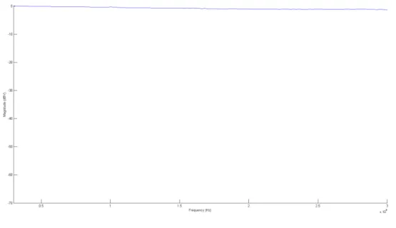
To implement the alternative shown on Figure 2-(b), the source signal must be a step signal so that
differentiating the time response of the DUT results in the impulse response of the system. In
addition, the rise time of the step must be short enough that the step can be considered ideal; for
comparison purposes, Figure 5 shows the frequency spectrum of the derivative of the response signal,
which must be close to the ideal case for the method to be valid, that is, a spectral band that is flat for
all frequencies. Since the step signal is not ideal, a high frequency decay can be seen on Figure 5, but
the smoothness of the response justifies the alternative implementation of figure 2-(b), as the result is
very close to ideal.
Fig. 5. Frequency domain information for the derivative of the input signal.
Tests were made with two bandpass filters, with central frequencies 925 MHz and 1065 MHz,
shown in figure 6. Time domain data was collected and processed with MATLAB software, and then
compared to data from a network analyser.
Fig. 6. 925MHz and 1065MHz filters used for testing.
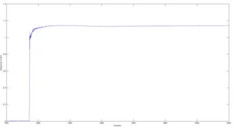
The time domain data from the response of the DUT is sent to the frequency domain through the
Fourier Transform discussed previously. This is the output signal of the system. The smoothed time
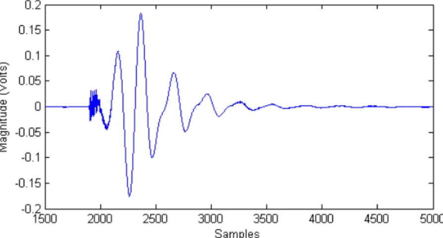
Fig. 7. Smooth time domain output data for the 925MHz filter.
Fig. 8. Smooth time domain output data for the 1065MHz filter.
The transfer function of the system can now be calculated. With the transfer function, the
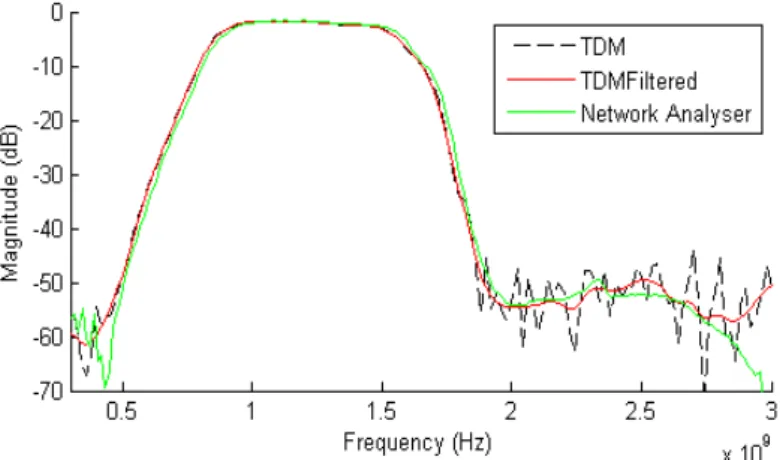
S-Parameters can be calculated as discussed in the previous section. Finally, figures 9 and 10 show the
frequency response data for both filters in black, as well as the smoothed result in red and the results
from a standard network analyser model in green, for comparison.
Fig. 9. Transmission Results for 925MHz filter. The green line shows the result from a vector network analyser, the dashed black line shows the result of the processing technique and the red line shows the result of the processing technique after
Fig. 10. Transmission Results for 1065MHz filter. The green line shows the result from a vector network analyser, the dashed black line shows the result of the processing technique and the red line shows the result of the processing technique
after mathematical filtering was performed.
Despite being close to ideal, the high-frequency decay in the derivative of the input signal shows
that there will be an increasing error in the output data at high frequencies: as it decays, the frequency
response rises due to equation 7. Another factor that can be seen from the unsmoothed dashed black
line is that the results become increasingly noisy at very low magnitudes (below -50 dB) due to the
computations reaching the noise floor of the DFT algorithm utilized; this can be seen more easily on
the 1065 MHz filter result, as it reaches lower magnitudes.
V. DISCUSSION
The results from the time domain analysis match with the results from the network analyser for the
entire operational band of both filters tested. It was observed that the noise in the time domain data is
an important factor in obtaining good results, and that time domain responses have a trend of being
extremely noisy at their start.
The precision for the pulse's rise time of the equipment used for the time domain data acquisition is
also an important factor to consider. With a more precise and faster equipment, not only the frequency
band for which the technique matches increases, but noise and errors are also reduced in magnitude.
The results shown in this paper are for TDT analysis only, that is, for the S21 and S12 parameters. The
technique is also applicable to TDR data and can also be employed for phase analysis of signals, but
concerns of noise and precision appear, as both reflection waves and phase detection are more
sensible to these errors.
In a future analysis, both TDR and phase information could be obtained by the use of advanced,
more precise, faster and less noisy equipment.
REFERENCES
[1] K. Kurokawa, “Power waves and the scattering matrix,” Microwave Theory and Techniques, IEEE Transactions on, vol. 13, no. 2, pp. 194_202,1965.
[9] D. Gorinevsky, ”Optimal estimate of monotonic trend with sparse jumps, ” in American Control Conference, 2007. ACC'07, pp. 1051-ᄃ1056, IEEE, 2007.
[10] S. M. Wentworth, Fundamentals of electromagnetics with engineering applications. Wiley, 2004.
[11] C. E. Shannon, ”Communication in the presence of noise, ” Proceedings of the IRE, vol. 37, no. 1, pp. 10-21, 1949.
[12] A. V. Oppenheim, A. S. Willsky, and S. H. Nawab, Signals and systems, vol. 2. Prentice-Hall Englewood Cliffs, NJ, 1983.
[13] K. Runtz and D. Hack,”A multistage dft-fft-czt approach for accurate e-cient analysis of sparsely distributed spectra,” in Electrical and Computer Engineering, 2002. IEEE CCECE 2002. Canadian Conference on”, vol. 1, pp. 127-132, IEEE, 2002.
[14] L. Rabiner, R. W. Schafer, and C. M. Rader, ” The chirp z-transform algorithm” Audio and Electroacoustics, IEEE Transactions on, vol. 17, no. 2, pp. 86-92, 1969.
[15] P. J. Pupalaikis, ”The relationship between discrete-frequency s-parameters and continuous-frequency responses, ” 2012.