www.the-cryosphere.net/10/2907/2016/ doi:10.5194/tc-10-2907-2016
© Author(s) 2016. CC Attribution 3.0 License.
Weichselian permafrost depth in the Netherlands: a comprehensive
uncertainty and sensitivity analysis
Joan Govaerts1, Koen Beerten1, and Johan ten Veen2
1SCKqCEN, Institute Environment-Health-Safety, Boeretang 200, 2400 Mol, Belgium
2TNO Geological Survey of the Netherlands, Princetonlaan 6, 35584 CB Utrecht, the Netherlands
Correspondence to:Joan Govaerts ([email protected])
Received: 25 February 2016 – Published in The Cryosphere Discuss.: 12 May 2016 Revised: 30 September 2016 – Accepted: 23 October 2016 – Published: 25 November 2016
Abstract.The Rupelian clay in the Netherlands is currently the subject of a feasibility study with respect to the storage of radioactive waste in the Netherlands (OPERA-project). Many features need to be considered in the assessment of the long-term evolution of the natural environment surround-ing a geological waste disposal facility. One of these is per-mafrost development as it may have an impact on various components of the disposal system, including the natural en-vironment (hydrogeology), the natural barrier (clay) and the engineered barrier. Determining how deep permafrost might develop in the future is desirable in order to properly address the possible impact on the various components. It is expected that periglacial conditions will reappear at some point dur-ing the next several hundred thousands of years, a typical time frame considered in geological waste disposal feasibil-ity studies. In this study, the Weichselian glaciation is used as an analogue for future permafrost development. Permafrost depth modelling using a best estimate temperature curve of the Weichselian indicates that permafrost would reach depths between 155 and 195 m. Without imposing a climatic gradi-ent over the country, deepest permafrost is expected in the south due to the lower geothermal heat flux and higher aver-age sand content of the post-Rupelian overburden. Account-ing for various sources of uncertainty, such as type and im-pact of vegetation, snow cover, surface temperature gradi-ents across the country, possible errors in palaeoclimate re-constructions, porosity, lithology and geothermal heat flux, stochastic calculations point out that permafrost depth during the coldest stages of a glacial cycle such as the Weichselian, for any location in the Netherlands, would be 130–210 m at the 2σ level. In any case, permafrost would not reach depths
greater than 270 m. The most sensitive parameters in
per-mafrost development are the mean annual air temperatures and porosity, while the geothermal heat flux is the crucial parameter in permafrost degradation once temperatures start rising again.
1 Introduction
diffi-cult to observe in the geological record. Therefore, numerical simulation seems to be the most suitable tool to estimate past and future permafrost depths and has been applied already in several case studies elsewhere in Europe (Deslisle, 1998; Grassmann et al., 2010; Kitover et al., 2013; Busby et al., 2015).
Many of the countries that experienced permafrost in the past, such as the Netherlands, Belgium, United Kingdom, France and Germany, are currently running feasibility stud-ies for the disposal of radioactive waste in deep geological repositories (Grupa, 2014). The concept of geological dis-posal is based on a multi-barrier system. Engineered barriers, consisting of steel components, concrete and/or bentonite are designed to contain the nuclear waste. Subsequently, the engineered barrier is placed in a natural barrier consisting of a low-permeability host rock that is situated at sufficient depth and located in a stable geological environment. Per-mafrost development may have an impact on various com-ponents of the disposal system, including the natural envi-ronment, the natural barrier and the engineered barrier. The hydrological cycle will completely change under permafrost conditions, up to the point where surface and subsurface hy-drology become completely independent, and groundwater flow is drastically changed (Weert et al., 1997). Furthermore, landscape, vegetation and thus the biosphere will be com-pletely different under permafrost conditions (Beerten et al., 2014). Hydraulic properties of aquifer sands and aquitard clays might be affected during permafrost conditions, espe-cially if accompanied by repeated freeze–thaw cycles (Oth-man and Benson, 1993; McCauley et al., 2002). Migration of radionuclides through the host rock may be altered and the mechanical properties of the engineered barriers may be affected due to freeze–thaw cycles (Busby et al., 2015). Pore-water chemistry might change due to outfreezing of salts, and gas hydrates may develop (Stotler et al., 2009). Finally, mi-crobial activity in the host rock will likely be affected. It is thus important to determine how deep permafrost will de-velop in order to properly address the possible impact on the various components. Thick and deep low-permeability clay formations are often good candidates for host rocks. The Ru-pelian clay, which is subcropping in most of the northwest-ern European countries mentioned above (Vandenberghe and Mertens, 2013), is considered in the Dutch geological dis-posal project (Onderzoeksprogramma eindberging radioac-tief afval, “OPERA”) as a candidate host-rock (Grupa, 2014). In the present northwestern European context it provides an interesting case study because it is distributed over a wide range of settings with respect to overburden thickness, lithol-ogy, porosity and geothermal heat flux.
Usually, uncertainties in permafrost modelling studies in the context of radioactive waste disposal are not addressed in a systematic way (e.g. Busby et al., 2015; Holmen et al., 2011; Hartikainen et al., 2010). The sensitivity of permafrost models is often assessed in terms of variations to single pa-rameters like porosity or surface temperature one at a time
(Kitover et al., 2013). These kinds of local sensitivity analy-ses (SAs) asanaly-sess the response of the model output to a small perturbation of single parameters, one at a time, around a nominal value. The main disadvantage of this method is that information about the sensitivity is only valid for this very specific location in the parameter space, which is usually not representative of the physically possible parameter space, and becomes problematic especially in the case of non-linear models. To overcome this problem, a global stochastic sensi-tivity analysis is used in this work, where multiple locations in the physically possible parameter space are evaluated at the same time.
In this paper, we will present permafrost depth calculations for a number of areas in the Netherlands that are represen-tative for a specific geological setting using a best estimate temperature curve for a glacial cycle that is analogous to the last glacial period (Weichselian). In addition, results from stochastic simulations will be presented that give an indica-tion of the probability of permafrost depths under a future glacial climate, taking into account various combinations of temperature, overburden lithology, porosity and geothermal heat flux. Furthermore, a sensitivity analysis is performed to identify the key model parameters that cause the uncertainty of the calculated permafrost depths. As such, the work per-formed in Govaerts et al. (2011), which was done for one potential site in the framework of the Belgian research pro-gramme on geological disposal, is taken a few steps further.
The results of the simulations can be used to assess if the foreseen depth of a future geological disposal facility in the Netherlands is sufficient to exclude possible adverse effects from the presence of developing permafrost. Until now, these kinds of simulations were not performed nationwide, and a more thorough uncertainty and sensitivity analysis adds to the robustness of the findings.
2 Mathematical and numerical model for permafrost growth and degradation
To describe heat transport in the subsurface of the Nether-lands, the following one-dimensional enthalpy conservation equation is used with heat transport only occurring by con-duction.
Ceq∂T
∂t + ∇ · −λeq∇T
=Q, (1)
whereCeqis the effective volumetric heat capacity (J K m3),
T is temperature (K),λeqis the effective thermal
conductiv-ity (W (m K)−1) and
Qis a heat source (W m−3).
and ice. To achieve this, the following volume fractions are defined:
θm=1−θ θf=θ·2, θi=θ−θf. (2)
The subscripts f, i and m account for the mixture between solid rock matrix (m), fluid-filled pore space (f) and ice-filled pore space (i). This mixture is characterized by poros-ityθ, and2denotes the fraction of pore space occupied by
fluid. As a result of the complicated processes in the porous medium, thawing cannot be considered as a simple disconti-nuity.2is generally assumed to be a continuous function of
temperature in a specified interval.
When a material changes phase, for instance from solid to liquid, energy is added to the solid. This energy is the latent heat of phase change. Instead of creating a temperature rise, the energy alters the material’s molecular structure. This la-tent heat of freezing and melting water,L, is 333.6 kJ kg−1
(Mottaghy and Rath, 2006).Ceqis a volume average, which
also accounts for the latent heat of fusion:
Ceq=θmρmcm+θfρf
cf +
∂2 ∂TL
+θiρi
ci+∂2
∂TL
, (3)
whereθis the volumetric content,ρequals density (kg m3),
and C is the specific heat capacity (J (K kg)−1). It includes additional energy sources and sinks due to freezing and melt-ing usmelt-ing the latent heat of fusion L for only the
normal-ized pulse around a temperature transition ∂2 ∂T (K
−1
). The
integral of ∂2
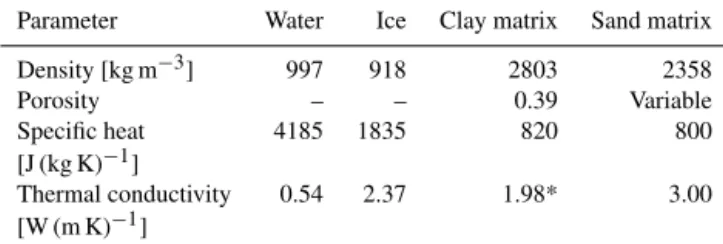
∂T must equal unity to satisfy the condition that pulse width denotes the range between the liquidus (thaw-ing) and solidus (freez(thaw-ing) temperatures of the porous soil. During cooling, solidus is that temperature at which most of the pore water of the soil is frozen. Between the solidus and liquidus temperatures, there will be a mixture of solid and liquid water phases within the soil matrix. Just below the liq-uidus temperature, there will be mostly liquid water phases. This approach is similar to the one used by Mottaghy and Rath (2006), Bense et al. (2009), Noetzli and Gruber (2009), Holmén et al. (2011) and Kitover et al. (2013). Values for the porosity, density and specific heat of the different com-ponents are given in Table 1.
The values of the specific heat of the Boom Clay matrix are obtained from Cheng et al. (2010). The equivalent, mass-based heat capacity then adds up to 1443 and 981 J (kg K)−1 for the fully unfrozen and frozen states respectively, obtained by using Eq. (3) and dividing by the bulk density of Boom Clay. This is in the same range as the values used in Marivoet and Bonne (1988) and Kömle et al. (2007) for clay sedi-ments. The value of the sand matrix is set to a value inside the ranges that are found for quartz minerals and sands (see Mallants, 2006 and references therein). For sandy soils, the
Table 1.Properties of the different components of the subsoil.
Parameter Water Ice Clay matrix Sand matrix
Density [kg m−3] 997 918 2803 2358 Porosity – – 0.39 Variable Specific heat 4185 1835 820 800 [J (kg K)−1]
Thermal conductivity 0.54 2.37 1.98* 3.00 [W (m K)−1]
∗This value has been chosen so the effective thermal conductivity equals 1.31 J (kg K)−1, which is the vertical thermal conductivity of Boom Clay obtained during the ATLAS study (Chen et al., 2010).
equivalent heat capacity adds up to 1319 and 937 J (kg K)−1 for the fully unfrozen and frozen states respectively when a porosity of 30 % is assumed.
In case of phase change at a single temperature, thermal conductivity is not continuous with respect to temperature. However, considering the freezing range in rocks, we use Eqs. (2) and (4) for taking into account the contributions of the fluid and ice phases. Since the materials are assumed to be randomly distributed, the weighting between them is re-alized by the square-root mean, which is believed to have a greater physical basis than the geometric mean (Roy et al., 1981).
λeq=θmpλm+θfpλf+θipλi
2
(4) Values for the thermal conductivity of the different compo-nents are given in Table 1.
The values of the thermal conductivity of the rock ma-trix of Boom Clay and sand are chosen in the same range of the values used by Bense et al. (2009) and Mottaghy and Rath (2006), who used respectively 4.0 and 2.9 W (m K)−1 for a generic sediment rock species.
For Boom Clay, the equivalent thermal conductivity then adds up to 1.31 and 2.03 W (m K)−1for fully unfrozen and frozen states respectively. The conductivity value of unfrozen Boom Clay is thus equal to the vertical conductivity obtained from the ATLAS 3 study (Cheng et al., 2010).
In sandy soils, the equivalent thermal conductivity is 2.05 and 2.80 W (m K)−1 for the fully unfrozen and frozen state respectively. The values are in the same range as the values found in Mallants (2006) and the references therein.
The heat transport equation is implemented in COMSOL Multiphysics’ Earth Science Module (2008), together with all the correlations for the thermal properties. Because the thermal properties differ between the frozen and unfrozen state, a variable2is created, which goes from unity to zero
for fully unfrozen to frozen. Therefore, the effective prop-erties switch with the phase through multiplication with2.
The switch in2from 0 to 1 occurs over the liquid-to-solid
interval (0.0 to−0.5◦C) using a fifth orderS-shaped
func-tion with a continuous second derivative without overshoot and takes on a value between 0 and 1. As such, in this model representation, the freezing process is determined only by the change in temperature. The dependency of the freezing point of water on pressure, salinity and the adsorptive and capillary properties of the soil is not taken into account in the present calculations.
Moreover, the freezing process is modelled using a gradual and not a sudden uptake and release of the latent energy, start-ing at 0◦C to ensure numerical stability. Ideally, this freez-ing interval should be kept as small as possible. However, decreasing the size of the interval will increase the compu-tational burden and compromise the numerical stability. The effect of the size of the freezing interval on the permafrost depth was previously investigated by Govaerts et al. (2011, Appendix A). It was shown that there is little influence on the resulting temperature profiles as the 50 % frozen iso-line (which corresponds to the centre temperature value of the liquid–solid interval) is nearly identical for all the values that have been tested in that study. The size of the liquid-to-solid temperature interval does not seem to have a significant impact on the retardation of the cold wave, a phenomenon also known as the zero curtain effect. In this study, the 0◦C isotherm, which corresponds to the 0 % frozen state, is used as the metric for permafrost depth.
2.1 Parameters, initial and boundary conditions used in the reference calculation
Permafrost development is dependent on atmospheric and surface boundary conditions, mostly air temperature and veg-etation, and subsurface properties such as lithology, poros-ity and geothermal heat flux. As such, it is the result of in-teractions between global changes (temperature) and local conditions (geology). The strategy adopted for this specific study consists of the following elements. First, we try to sim-ulate a future glacial climate using the Weichselian glaciation (115–11 ka) as an analogue. Various temperature estimates are available for this glacial period, many of them being de-rived from palaeoclimatological archives in Belgium and the Netherlands. The forcing temperature is allowed to change temporally at the upper boundary but held spatially uniform for a given time step. Subsequently it will be used to force the permafrost model, which is fragmented into different repre-sentative polygons. The initial condition of the model is the steady state temperature profile based on the present day tem-perature gradient.
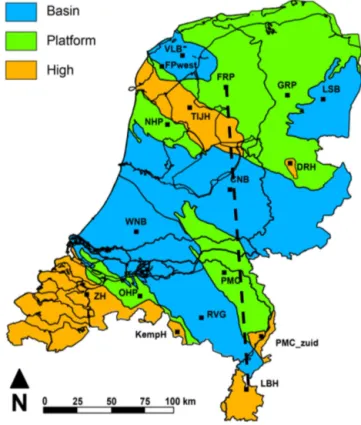
The thickness of subsurface units and their lithofacies dis-tribution are considered relevant for permafrost modelling as this affects porosity and the effective thermal properties. The selection of the different areas for permafrost modelling is based on the presence of 17 structural elements, includ-ing six highs, five basins and six platforms (Fig. 1). The rationale is that these structural elements delineate differ-ences in thickness and depths of both Mesozoic and
Ceno-Figure 1. Structural elements in the Dutch subsur-face. LBH=Limburg High, RVG=Ruhr Valley Graben, KempH=Kempisch High, ZH=Zeeland High, OHP=Oosterhout Platform, PMC=Peel-Maasbommel, PMC_zuid= Peel-Maasbommel High, WNB=West Netherlands Basin, CNB=Central Netherlands Basin, DRH=Drenthe High, NHP=Noord Holland Platform, TIJH=Texel-IJsselmeer High, FRP=Friesland Platform, FP (west)=Friesland Platform, VLB=Vlieland Basin, GRP=Groningen Platform, LSB=Lower Saxony Basin. Dashed line refers to the profile shown in Fig. 7.
zoic subsurface units. Subsequently, a geological (property) model was constructed based on the surfaces of the deep ge-ological model (DGM) shallow subsurface model. For each unit, vertical grid cells with a surface of 250 m×250 m
and a height equal to the thickness of the unit were con-structed. These grid cells were populated with the parame-ters described before. Subsequently, all parameparame-ters were av-eraged over the vertical interval overlying the Rupel Forma-tion (the overburden). The research area is subdivided into several polygons with dimensions ranging roughly between 9 km×15 km and 110 km×140 km. The midpoint positions
of the various polygons are plotted in Fig. 1.
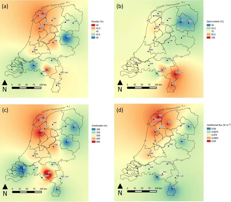
in-Figure 2. (a)Averaged mid-depth porosity variability of the post-Rupelian overburden,(b)distribution of the average sand content in the post-Rupelian overburden,(c)depth of the top of the Rupel Formation, also representing the thickness of the overburden (m),(d)spatial distribution of geothermal heat flux values (W m3). The flux is significantly higher in the (north)west than the (south)east of the country.
cluded, but rather serves to highlight regional trends over the Netherlands.
2.2 Porosity, lithology and overburden thickness An important parameter for permafrost modelling is poros-ity. Porosity is directly linked with water content as full sat-uration is assumed. Consequently, thermal conductivity and the equivalent heat capacity of the soil correspond with these conditions (see Table 1 and Eq. 3). A porosity value is as-signed to each of the lithostratigraphic units defined in the Digital Geological Model (DGM; Gunnink et al., 2013) of the shallow Dutch subsurface. The hydrogeological model
REGIS (Vernes and van Doorn, 2005) provides a further sub-division and includes both aquifers (sand) and non-aquifer layers (clay). Using the REGIS information a percentage of clay vs. sand for each of the DGM units can be calculated. Based on a relatively small number of porosity measure-ments of the sand and clay layers in the stratigraphic interval above the Rupel Formation, a best fit, generally applicable porosity–depth relationship was established for all sandy and clayey depositional facies of the various units. This allows for making porosity predictions in non-studied domains.
50 %. The lowest values are found in the southeast (Ruhr Val-ley Graben, polygon RVG) and the northwest. The porosity is influenced by two other parameters: lithology and burial depth. The thicker the post-Rupelian overburden, the deeper the mid-depth for which the porosity is determined, and thus the lower the porosity. Lithology also has an influence on porosity because on average, clay has a higher porosity than sand. As such, the porosity map is a mirror image of a com-bination of lithology and overburden thickness. Note that the depth to the top of the Rupel Formation is representative for the total overburden depth, which is strongly coupled to the tectonic setting, i.e. thick in basins and grabens and relatively thin on structural highs (Figs. 1 and 2). Lithofacies (given as sand percentage) seem to be linked to certain structural el-ements. Notably in the southeastern Netherlands, the sand content is very high, reaching more than 80 % in the RVG and adjacent areas. These areas acted as traps for a thick se-ries of Neogene continental sands.
2.3 Upper boundary condition: temperature evolution of a future glacial cycle
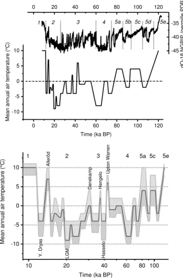
The temperature curves and data used in this study are shown in Fig. 3. Best estimates for the mean annual air temperature (MAAT) during MIS5 (marine isotope stage 5) are based on pollen data from van Gijssel (1995), but replotted against a more recent chronostratigraphic framework for the Weich-selian glaciation (see e.g. Busschers et al., 2007). The main features of the MIS5 climate are the relatively mild stadials 5b and 5d, with a MAAT of−2◦C, and the relatively cold
in-terstadials 5c and 5a, with a MAAT of+4◦C. The first period
with continuous permafrost development in the Netherlands would have been MIS4, with MAAT values dropping to as low as−4◦C (threshold for discontinuous permafrost) and
even−8◦C (threshold for continuous permafrost) for the end
of MIS4. These values are based on periglacial deformation phenomena (e.g. ice-wedge casts and large-scale involutions) in the shallow subsoil and their present-day distribution in ar-eas of stable continuous permafrost (Vandenberghe and Pis-sart, 1993; Huijzer and Vandenberghe, 1998; Vandenberghe et al., 2014). The following MIS3 is characterized by a some-what milder climate, showing less periglacial deformation of the subsoil. Analysis of flora and fauna preserved within MIS3 sediments, and the type and nature of periglacial de-formation shows that some interstadials might have reached a MAAT between 0 and +6◦C (e.g. Upton Warren,
Hen-gelo and Denekamp interstadials; Huijzer and Vandenberghe, 1998; Busschers et al., 2007; van Gijssel, 1995), and several stadials would have reached an MAAT as low as−4◦C (e.g.
Hasselo stadial; Busschers et al., 2007). Subsequently, the climate evolves towards the Late Glacial Maximum (LGM), which is situated in MIS2. Data for this stage are mainly derived from Renssen and Vandenberghe (2003) and Buy-laert et al. (2008) and are based on the presence and type of periglacial deformation phenomena. The MAAT for the
20 40 60 80
10 100 -10 -5 0 5 10 Y. Drya s Al leröd LGM Denek amp Hengel o Has s el o
1 2 3 4 5a 5c
Me an an nu al a ir te mp er atu re (°C)
Time (ka BP)
5e
Upton W
arr
en
0 20 40 60 80 100 120
-10 -5 0 5 10 15 20
0 20 40 60 80 100 120
-70 -65 -60 -55 -50 -45 -40 -35 Mean annual air tempe ratur e (°C)
Time (ka BP)
5d 5b
1 2 3 4 5a 5c 5e
dO -18 NGRIP (per mi lle PDB )
Figure 3. Top: best estimate temperature evolution for the We-ichselian glaciation, which is taken as an analogue for a future glacial climate in permafrost calculations. The curve is based on data from van Gijssel (1995), Huijzer and Vandenberghe (1998), Renssen and Vandenberghe (2003), Busschers et al. (2007) and Buylaert et al. (2008). Marine isotope stages (numbering 1 to 5e) are taken from Busschers et al. (2007) and references therein. The oxygen isotope curve is reproduced from the North Green-land Ice Core Project (NGRIP) (2004) data. Bottom: upper and lower bound values for stochastic permafrost calculations on a log-arithmic timescale. MIS5e is equivalent to the Eemian interglacial, while MIS1 corresponds to the Holocene (present interglacial). Y. Dryas=Younger Dryas.
period between 28 and 15 ka would not have exceeded 0◦C, while some periods show MAAT values as low as−8◦C. The
end of MIS2 is characterized by a stepwise trend towards global warming, showing significant variations between in-terstadials (Alleröd) and stadials (Younger Dryas). Finally, present-day MAAT values of around+10◦C are attributed
to MIS1.
esti-mate temperature evolution for the Weichselian glaciation used as an analogue, a minimum and maximum tempera-ture distribution for each time frame is determined, which will be randomly sampled to produce various combinations of upper and lower bound MAAT values in the stochas-tic uncertainty analyses. Different sources of uncertainty are thus taken into account, such as the reliability of the palaeotemperature proxy, the transferability towards a fu-ture glacial climatic cycle, temperafu-ture gradients across the country and atmosphere–soil temperature coupling. Lower bound estimates are set ca. 3–4◦C lower than the best es-timate. This range allows for uncertainty with respect to the palaeotemperature proxy in the case of discontinuous per-mafrost, which might exist up to MAAT values as low as
−8◦C before it turns into continuous permafrost (Huijzer
and Vandenberghe, 1998). For the coldest periods, such as the LGM, the lower bound MAAT was set to−11 or 21◦C
below the present day MAAT. This allows the possibility of a future glacial colder than the Weichselian analogue (e.g. the Saalian, when the Fennoscandian ice-sheet margin reached the Netherlands; Svendsen et al., 2004). Furthermore, a 21◦C temperature drop for the LGM is in line with the coldest es-timate reconstructions for low lying areas in Great Britain (Busby et al., 2015). As a result, the MAAT remains below 0◦C throughout much of the glacial cycle, except for several short interstadials, such as the Alleröd.
The upper bound is based on a warm reconstruction of the Weichselian climate, which is based on a pollen sequence in sediments from the crater lake at La Grande Pile, situated ca. 500 km south of Amsterdam at an altitude of ca. 350 m (Guiot et al., 1989). The mean MAAT estimate obtained in that study is used here as an absolute maximum scenario for the Weichselian glaciation in northwestern Europe given its location. The upper bound for the time period around 20 ka, for which the pollen record gives no solution, is set to−4◦C
(or 14◦C below the present-day MAAT), because we assume that at least discontinuous permafrost would have developed in northwestern Europe around that time period. This value is slightly lower than globally reconstructed temperatures for the LGM in northwestern Europe as proposed by Annan and Hargreaves (2013) using climate modelling and proxy data.
The temperature data presented here are directly used as soil surface temperature data. However, vegetation, snow or ice would act as a shield against penetration of cold air and hamper the evolution of permafrost with depth. The effect of vegetation and snow can be addressed using the concept of freezing and thawing nfactors, which are equal to 1 in the
case of no vegetation or snow and gradually decrease with vegetation type and snow thickness (Lunardini, 1978). Dur-ing a Weichselian glacial cycle as the one presented here, the shielding effect of snow would increase the mean annual soil surface temperature (MAST) by 2 to 5◦C with respect to the MAAT (northern Belgium; Govaerts et al., 2011). Departing from the best estimate temperature curve, this range is almost entirely covered by the uncertainty range (Fig. 3).
It has to be mentioned that the model neglects subsur-face hydrology such as the vadose zone and groundwater flow. During very cold stadials, infiltration would probably be so low that the groundwater table would be significantly lower. Unsaturated soil slows down permafrost development because of the difference in thermal conductivity between air and water. Full saturation of the pore space is adopted in the present calculations, aiming at keeping the model con-servative with respect to neglected processes. Next, ground-water flow is neglected but it is evident that this would slow down the speed of permafrost development as well be-cause of the redistribution of heat (Kurylyk et al., 2014). Fi-nally, outfreezing of pore water salt would lower the speed of permafrost development because more heat needs to be extracted to freeze water with elevated salt concentrations (Stotler et al., 2009).
2.4 Lower boundary condition: geothermal heat flux For each of the 17 polygons, the mid-depth temperature and the surface temperature were used to calculate the temper-ature gradient. These data are then used to calculate the geothermal heat flux using the averaged thermal conduc-tivity values of the sandy overburden (Fig. 2d). Generally speaking, the country is split up between a southeastern part with lower values of the geothermal heat flux (0.06– 0.07 W m−3) and a northwestern part with higher flux values (up to 0.09 W m−3). It is interesting to note that this pattern follows the pattern of recent differential tectonic land move-ment as calculated by Kooi et al. (1998). The higher flux val-ues in the northwest can also be linked to higher mid-depth temperatures in that area. These in turn are the result of the presence of Zechstein salt layers that have a relatively high thermal conductivity (ca. 4 W (m K)−1; Bonté et al., 2012). 2.5 Model domain, boundary conditions and
computational settings
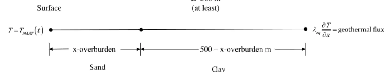
The upper part of the one-dimensional domain is modelled as sandy soil for each of the 17 polygons as deep as the overbur-den reaches. The total vertical length of the one-dimensional lithological domain is then extended to at least 500 m with clay material, in case the overburden does not reach this depth. This implies assuming that the Rupelian layers un-derlying the overburden are sufficiently thick to bridge the distance from the bottom of the overburden to a depth of 500 m. The lower boundary condition needs to be imposed at a distance sufficiently far from the top to avoid artificial, numerical interaction with the surface temperature boundary condition. This is illustrated, together with the boundary con-ditions, in Fig. 4. Material parameters are held constant along the domain length for each soil type.
Surface
500 – x-overburden m
C lay L=500 m
(at least)
geothermal flux
eq T x
Sand
x-overburden
MAAT TT tFigure 4.Model domain and boundary conditions.
mesh of 500 equidistant elements is chosen as an optimal setting for the final simulations. Absolute and relative toler-ances for convergence within each timestep are set to 1e-4. The COMSOL software adapts the size of the timestep in order to fulfill this requirement.
2.6 Stochastic uncertainty and sensitivity analysis 2.6.1 Uncertainty analysis
As an integral part of a safety case file, supporting calcula-tions for radioactive waste disposal often involves the anal-ysis of complex systems. Various types of uncertainty af-fect the results of the evaluations. An overview of the treat-ment of uncertainties in the disposal programmes of several European countries has been compiled within the PAMINA project (Marivoet et al., 2008).
The nature of the uncertainty can be stochastic (or aleatory) or subjective (or epistemic). Epistemic uncertainty derives from a lack of knowledge about the adequate value for a parameter, input or quantity that is assumed to be constant throughout model analysis. In contrast, a stochas-tic model will not produce the same output when repeated with the same inputs because of inherent randomness in the behaviour of the system. This type of uncertainty is termed aleatory or stochastic.
In general a distinction is made between three sources of uncertainty: uncertainty in scenario descriptions, including the evolution of the main components of the repository sys-tem; uncertainty in conceptual models; uncertainty in param-eter values.
Although both types and even sources of uncertainties can-not be entirely separated, the work in this report deals mostly with subjective (or epistemic) uncertainties, which are re-flected in the uncertainties in parameter values.
Parameters, initial and boundary conditions for mathemat-ical models are seldom known with a high degree of cer-tainty. The study of parameter uncertainty is usually subdi-vided into two closely related activities referred to here as uncertainty analysis and sensitivity analysis, where (i) certainty analysis (UA) involves the determination of the un-certainty in analysis results that derive from unun-certainty in input parameters and (ii) sensitivity analysis (SA) involves the determination of relationships between the uncertainty in
analysis results and the uncertainty in individual analysis in-put parameters. SA identifies the parameters for which the greatest reduction in uncertainty or variation in model output can be obtained if the correct value of this parameter could be determined more precisely.
To this end, a Monte Carlo simulation is based on per-forming multiple model evaluations using random or pseu-dorandom numbers to sample from probability distributions of model inputs. The results of these evaluations can be used to both determine the uncertainty in model output and per-form SA. The popular and robust Monte Carlo (MC) method in combination with the efficient Latin hypercube sampling (LHS) is used here and is described in several review pa-pers and textbooks (e.g. Marino et al., 2008; Helton, 1993). LHS requires fewer samples than simple random sampling and achieves the same level of accuracy.
2.6.2 Implementation
Table 2. Parameters and associated ranges used in the global UA and SA., T1 to T26, are used to control the magnitude of the various temperature plateaus during the Weichselian temperature cycle (Fig. 3), ranging from−11◦C for the lowest and+11◦C for the highest.
Parameter Minimum Maximum Mode Simulation time frame (ka)
Porosity [–] 0.2 0.7 0.45 All
Fraction of sand [–] 0.1 1 0.75 All
Geothermal heat flux [W m−3] 0.033 0.115 0.060 All
Overburden thickness [m] 20 1500 500 All
Initial temperature gradient [K m−1] 0.022 0.033 0.028 Initial condition
T1 [K] 281.15 284.15 283.15 0–11.5
T2 [K] 269.15 273.15 271.15 12–13
T3 [K] 273.15 281.15 277.15 14–14.5
T4 [K] 269.15 273.15 271.15 15–15.5
T5 [K] 273.15 283.15 277.15 16–16.5
T6 [K] 265.15 273.15 269.15 17.5–18
T7 [K] 269.15 275.15 273.15 18.5–19
T8 [K] 263.15 269.15 265.15 19.5–21
T9 [K] 271.15 275.15 273.15 21.5–22
T10 [K] 270.15 275.15 272.15 22.5–25
T11 [K] 277.15 281.15 279.15 26–28
T12 [K] 264.15 271.15 269.15 30–31
T13 [K] 273.15 277.15 275.15 32–36
T14 [K] 266.15 271.15 269.15 37–37.5
T15 [K] 271.15 277.15 273.15 38–41
T16 [K] 267.15 271.15 269.15 42–43
T17 [K] 263.15 269.15 265.15 44–49
T18 [K] 265.15 269.15 268.15 50–55
T19 [K] 262.15 269.15 264.15 60–65
T20 [K] 269.15 275.15 272.15 68–71
T21 [K] 265.15 271.15 270.15 72–75
T22 [K] 269.15 275.15 271.15 80–85
T23 [K] 265.15 271.15 269.15 89–92
T24 [K] 277.15 283.15 280.15 93–102
T25 [K] 265.15 271.15 269.15 105–108
T26 [K] 281.15 284.15 283.15 120
2.6.3 Parameter Ranges
The stochastic simulations give an indication of the proba-bility of nationwide permafrost depths under a future glacial climate, taking into account various combinations of tem-perature, overburden lithology, porosity and geothermal heat flux.
A proper quantification of uncertainties in the form of probability density functions (PDFs) is an essential part of the uncertainty management and a prerequisite for proba-bilistic uncertainty and sensitivity analysis. As the actual knowledge about the statistical distribution of the parameters in question is limited, it is only possible to estimate a mini-mum, a maximum and a most probable value. In this case the triangular distribution is the most appropriate expression of the state of the knowledge (Bolado et al., 2009).
The parameters that are investigated in the stochastic anal-ysis are shown in Table 2. Their minimum, maximum and mode values are used to build a triangular probability den-sity function, which is sampled in the stochastic analysis. T1
to T26 are variables that are used to control the magnitude of the various temperature plateaus during the Weichselian tem-perature cycle. This allows to account for the actual parame-ter uncertainty for temperature as well as nationwide spatial parameter variability.
2.6.4 Sensitivity analysis
A wide range of SA methods exists but can generally be clas-sified into Local and Global techniques. Local SA will be assessing the response of the model output to a small per-turbation of single parameters (the so called one at a time method) around a nominal value. The main disadvantage of this method is that information about the sensitivity is only valid for this very specific location in the parameter space only, which is usually not representative of the physically possible parameter space, which becomes problematic espe-cially in the case of non-linear models.
possi-Figure 5.Top: best estimate permafrost progradation during a sim-ulation of the Weichselian glaciation cycle for the FRP polygon. Bottom: idem, for the LBH polygon. These two polygons (FRP and LBH) are at the low and high end of the resulting permafrost depths respectively.
ble parameter space are evaluated at the same time. The most frequently used global techniques are implemented using Monte Carlo simulations and are therefore called sampling-based methods. Global SA with regression-sampling-based methods rests on the estimation of linear models between parame-ters and model output. For linear trends, linear relationship measures that work well are the Pearson correlation coeffi-cient (CC), partial correlation coefficoeffi-cients (PCCs) and stan-dardized regression coefficients (SRC; Helton, 2005). In this study, the SRC will be used.
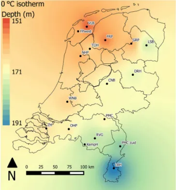
Figure 6.Interpolated best estimate maximum permafrost depth map for the 0◦C isotherm. The pore water is assumed to be com-pletely in the liquid phase.
3 Results
3.1 Permafrost development during a Weichselian temperature cycle – reference case
The definition of permafrost applied here is ground that remains at or below 0◦C for at least 2 consecutive years (French, 2007). The 0◦C isotherm is chosen as a conservative estimate of the permafrost front as explained earlier. Due to the choice of a gradual phase change between 0 and−0.5◦C,
a soil at−0.25◦C corresponds to a mixture of 50 water and
50 % ice.
The progradation fronts (i.e. the location where the tem-perature reaches 0,−0.25 and−0.5◦C, and corresponding
with 0, 50 and 100 % frozen soil respectively) for the FRP and LBH polygons are shown as a function of time (Fig. 5). The permafrost front penetrates about 155 to 195 m into the subsoil depending on the location, as a result of extremely low mean annual air temperatures during the final phase of MIS4 (early Pleniglacial) and the middle part of MIS2 (late Pleniglacial).
Figure 7.Simulated depth for different freezing states along a N–S transect from polygon centre FRP in the north to LBH in the south. See Fig. 1 for location of the profile.
the location where 0◦C is reached ranges from 155 to 195 m. The spatial variability in permafrost depth is further illus-trated along a N–S transect, from polygon centre FRP (Fries-land Platform) in the north to LBH (Limburg High) in the south (Fig. 7).
Somewhat surprisingly, the calculated permafrost depth would be about 40 m less in the north. Intuitively, one would expect permafrost to reach greater depths in the north, be-cause of the inferred temperature gradient over the coun-try. As stated above, the forcing temperature was assumed to be spatially homogeneous for a given time step across the study area, such that the results can be interpreted solely in terms of subsurface properties. The spatial pattern of maxi-mum permafrost depth is in fair agreement with the pattern of geothermal heat flux, as shown in Fig. 2, and a relation-ship with the weight fraction of sand can be observed as well. This seems logical since a higher geothermal heat flux im-poses a stronger resistance against the intrusion of subzero temperatures into the soil. A higher sand fraction facilitates permafrost growth, as a sand matrix has a higher thermal conductivity, which allows a more rapid extraction of ther-mal energy towards the surface during cold periods. Thus, assuming a constant temperature evolution over the Nether-lands, geothermal heat fluxes, and to a lesser extent sand per-centage, seem to be the determining factor in explaining the N–S variability of the maximum permafrost depth. Parame-ter sensitivity will be addressed in more detail in the section on the sensitivity analysis.
3.2 Results of the uncertainty analysis
The uncertainty analysis translates the uncertainty on the in-put parameters into an uncertainty on the permafrost depth (0◦C isotherm). The results are shown in Fig. 8. The
me-Figure 8.All percentiles of permafrost front penetration depth dur-ing a stochastic nationwide simulation of the Weichselian glacia-tion.
dian values of the maximum permafrost depth at a time of 20 ka are about 150 m, while the most conservative parame-ter combinations result in permafrost fronts going as deep as 280 m. Note that maximum permafrost depth for the 95–100 percentiles occurs after the thermal minimum for the cold phase around 60 ka BP, and not during the LGM (20 ka BP). This is caused by a number of simulations in which the ran-dom combination of cold temperatures in the period of 80 to 60 ka BP results in a very long and continuously cold pe-riod with temperatures ranging from−4 to−11◦C. The
dif-ference between the 5 % and 95 % percentiles (2σ )is about
80 m, which is quite high given the relatively low number of parameters.
3.3 Results of the sensitivity analysis
The goal of this sensitivity analysis (SA) is to determine the relationships between the uncertainty in output and the un-certainty in individual input parameters. SA identifies the pa-rameters for which the greatest reduction in uncertainty or variation in model output can be obtained if the correct value of this parameter could be determined more precisely. The results are analysed by looking at the evolution of the SRC and PCC coefficients. PCC and SRC provide related, but not identical, measures of the variable importance. If input fac-tors are independent, PCC and SRC give the same ranking of variable importance. This is the case in the present study, and we will focus on the SRC to discuss the sensitivity analysis. A positive correlation coefficient (SRC and/or PCC) means that a higher value of the parameter will cause a larger per-mafrost depth and vice versa.
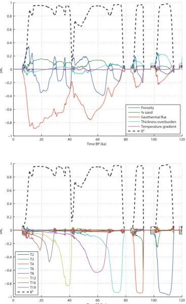
It can be seen in Fig. 9 that the R2 values are close to
0 20 40 60 80 100 120 −1
−0.8 −0.6 −0.4 −0.2 0 0.2 0.4 0.6 0.8 1
Time BP [ka]
SRC
T2 T3 T4 T6 T8 T12 T16 T19 R²
0 20 40 60 80 100 120
−1 −0.8 −0.6 −0.4 −0.2 0 0.2 0.4 0.6 0.8 1
Time BP [ka]
SRC
Porosity % sand Geothermal flux Thickness overburden Temperature gradient R²
Figure 9.SRCs as a function of time for a global sensitivity study of permafrost progradation during a Weichselian glaciation (top: phys-ical parameters, bottom: selected set of temperature parameters T1 to T26, which are variables that are used to control the magnitude of the various temperature plateaus during the Weichselian temper-ature cycle).
for most of the uncertainty in the permafrost depth, and the model is behaving in a linear way.
The SRC indicates that the geothermal heat flux is the most important parameter, aside from temperature forcing. It is in-teresting to note that during permafrost growth (e.g. around 90 ka) the geothermal heat flux is equally as important as the porosity. However, when the surface temperature again rises and the permafrost starts to degrade, the geothermal heat flux acts as the main driving force of the thawing process at the base of the permafrost, resulting in a decrease of the per-mafrost depth.
During the course of simulation time, correlation coeffi-cients can change their sign. During permafrost growth, at the
initial phase of a subzero temperature period, a higher poros-ity will hamper permafrost growth. Because of the larger ef-fective heat capacity, a larger pore water content means that a larger amount of energy needs to be removed from the sub-soil in order to cool it down and to induce a phase change of the total amount of pore water. A larger water content also de-creases the total effective thermal conductivity, which slows down the extraction of thermal energy towards the surface. Thereafter, during the subsequent warmer period, a higher ice content will require a larger amount of heat to be sup-plied to thaw the permafrost.
The sand fraction shows a relatively strong, positive influ-ence on permafrost depth, which confirms the findings of the nationwide simulation. Compared to clay, sand has a higher thermal conductivity, which will cause a more rapid cooling of the subsurface during cold periods.
The overburden thickness only seems to play a role during moderately cold periods (e.g. MIS 5b and 5d). If the overbur-den thickness is lower than 500 m, the remaining part of the domain is repleted with Boom Clay type material, which has a slightly lower thermal conductivity than the often sandy overburden, which slows down permafrost formation. This only seems to be of any importance in periods when the sur-face temperature is only slightly below the freezing point. Later, when the cold periods become more extreme (e.g. MIS 2), the difference in thermal conductivity at the clay–sand in-terface plays a less prominent role, and the other parameters become more significant.
Finally, it is no surprise that, being the driving force in the formation of a permafrost, the surface temperature is crucial at the time it is imposed on the computational domain (Fig. 9; in order not to overcrowd the figure, only 8 of the 26 temper-ature variables are shown). It is important to note that a spe-cific correlation coefficient becomes larger when that tem-perature is maintained for a longer period (e.g. T2 and T4). Closer to the present, the dynamics of the temperature evolu-tion during the Weichselian are better captured in the proxy data, which translates itself to a more detailed temperature evolution during the last 50 ky (T12–T26). Subsequently, this makes the individual temperature parameters seem less im-portant compared to the earlier temperatures, which can be seen as an artefact induced by the dynamics of the tempera-ture curve.
4 Discussion
The best estimate permafrost depth values of 155–195 m (0◦C isotherm) calculated here for the Weichselian glacia-tion in the Netherlands are somewhat lower than the 200 m that was obtained by Govaerts et al. (2011) using the same model and the same temperature curve. In the latter study, a lower porosity was used (down to 30 %), which favours the development of permafrost and thus explains the deeper permafrost. We now compare the results to other permafrost depth modelling results for NW Europe during the Weich-selian or a future analogue from Delisle (1998), Grassmann et al. (2010), Hartikainen et al. (2010), Holmén et al. (2011), Kitover et al. (2013) and Busby et al. (2015). These differ-ent modelling exercises revealed quite contrasting permafrost depths for the LGM, which is not surprising given that dif-ferent approaches and parameter values were used with re-spect to palaeotemperatures, duration of cold phases, sub-soil thermal properties, porosity, heat flux, ice advance, etc. The values derived from the different studies range between ca. 100 and ca. 300 m for a western European context, be-ing site- or non-site specific. Kitover et al. (2013) used an extended cold period of unknown duration and a MAAT of
−8◦C to produce steady-state continuous permafrost
reach-ing 300 m depth. Holmén et al. (2011) calculated a median permafrost depth for northwestern France of ca. 120 m us-ing a MAAT of−6◦C for the coldest peak during a future
Weichselian analogue. The value of 100 m from Delisle et al. (1998) is based on a relatively high MAAT of−7◦C for
the LGM during a very small time period at around 18 ka. Furthermore, that study used a fairly high geothermal heat flux, 60 mW m−3, as is the case for the study by Govaerts et al. (2011). The latter however used a lower MAAT (−9◦C)
for the LGM, persisting for 2000 years and preceded by al-ready very cold temperatures in the millennia before. Similar permafrost depths were obtained in the study by Grassman et al. (2010) for northern Germany covering the last 1 My. The maximum depth of 300 m for the permafrost base was realized during a cold peak around 400–450 ka with a mean annual ground surface temperature of−10◦C and a heat flux
of 50 mW m−2. Busby et al. (2015) calculated that for an ex-treme cold climate, based on the last glacial–interglacial cy-cle in Great Britain, maximum permafrost would vary be-tween 180 m (South Midlands) and 305 m (Southern Up-lands). The largest value of 305 m was obtained using an MAAT of ca. −20◦C for the coldest peak, which is about
8◦C lower than the one used in the present study. Note that in the coldest Southern Uplands scenario ice-sheet advance was considered during the glacial cycle, which has a shielding ef-fect on atmosphere–soil coupling. However, as only ground temperature was modelled by Busby et al. (2015), they could not make any statements about ice formation or the depth that partially or completely frozen ground might penetrate. Har-tikainen et al. (2010) also defined several permafrost cases with maximum modelled permafrost depths (0◦C isotherm)
of 260 and 390 m respectively for the Forsmark site in Swe-den.
The stochastic approach applied in this study combines a large range of parameter values and boundary conditions. Interestingly, this results in a permafrost depth distribution ranging between 100 and 270 m for the LGM. This win-dow seems to cover any of the calculated permafrost depths mentioned by previous studies. Some extreme values for the British Isles and Sweden that go beyond the thickest per-mafrost calculated in the present study are basically caused by much lower MAAT values for the coldest glacial peaks. Indeed, some of the remaining uncertainties are the duration and minimum MAAT values adopted for these cold peaks. Temperature reconstructions, based on periglacial deforma-tion phenomena, show that the MAAT during the LGM in the Netherlands would have been equal to or lower than−8◦C.
In our coldest scenario, we adopted a value of−11◦C that
would last for about 2000 years. To some extent these min-imum scenario values remain somewhat arbitrary, and the question is how much they should be lowered in order to cover any possible future glacial scenario. Notwithstanding these remaining uncertainties, so far the 300 m depth may be regarded as a maximum value because the model is con-servative with respect to vegetation and snow cover, ground-water flow and the depth of the unsaturated zone. These con-tributing factors would all push permafrost towards shallower depths. Note that in the OPERA-project the long term safety of a generic repository in the Boom Clay at a generic depth of 500 m will be assessed (Verhoef and Schröder, 2011). Fu-ture research should focus on defining an absolute minimum value for the MAAT used in permafrost calculations. It is also noted that the geothermal gradient, as used here for geother-mal heat flux calculation, might not be in equilibrium yet with present-day climatic conditions (ter Voorde et al., 2014). This should be taken into account in future permafrost mod-elling work.
5 Conclusions
and 210 m at the 2σ level. In any case, permafrost would
not reach depths greater than 280 m. The most sensitive pa-rameters in permafrost development are the mean annual air temperatures and porosity, while the geothermal heat flux is the crucial parameter in permafrost degradation once temper-atures start rising again. The permafrost depth distribution presented here encompasses many of the previously calcu-lated values for other contexts. Furthermore, the uncertainty analysis in which a wide range of parameter values are con-sidered makes the results presented here directly relevant for any western European lowland location with a sedimentary overburden.
The calculations presented here are robust and conserva-tive.
6 Data availability
Input data can be accessed at http://bit.ly/2fjtYxP.
Acknowledgements. The present work has been funded by
COVRA, the Dutch Central Organisation for Radioactive Waste. The findings and conclusions in this paper are those of the authors and do not necessarily represent the official position of COVRA. We thank the co-editor-in-chief Stephan Gruber for the critical re-view of the originally submitted paper. We also want to express our gratitude to Daniella Kitover and the anonymous reviewer for their helpful suggestions and comments on the discussion paper. Edited by: S. Gruber
Reviewed by: D. Kitover and one anonymous referee
References
Annan, J. D. and Hargreaves, J. C.: A new global reconstruction of temperature changes at the Last Glacial Maximum, Clim. Past, 9, 367–376, doi:10.5194/cp-9-367-2013, 2013.
Bense, V. F., Ferguson, G., and Kooi, H.: Evolution of shallow groundwater flow systems in areas of degrading permafrost, Geophys. Res. Lett., 36, TL22401, doi:10.1029/2009GL039225, 2009.
Berger, A. and Loutre, M. F.: An Exceptionally Long Interglacial Ahead?, Science, 297, 1287–1288, 2002.
Beerten, K., De Craen, M., and Leterme, B.: Long-term evolution of the surface environment of the Campine area, northeastern Bel-gium: first assessment, in: Clays in Natural and Engineered Bar-riers for Radioactive Waste Confinement, edited by: Norris, S., Bruno, J., Cathelineau, M., Delage, P., Fairhurst, C., Gaucher, E. C., Höhn, E. H., Kalinichev, A., Lalieux, P., and Sellin, P., Geo-logical Society, London, Special Publications, 400, 33–51, 2014. BIOCLIM Deliverable D3: Global climatic features over the next million years and recommendation for specific situa-tions to be considered, Modelling Sequential Biosphere Sys-tems under Climate Change for Radioactive Waste Disposal, A project within the European Commission 5th Euratom Frame-work Programme Contract FIKW-CT-2000-00024s, available at: http://www.andra.fr/bioclim/documentation.htm (last access: 20 February 2016), 2001.
Bolado, R., Badea A., and Poole, M.: Review of expert judgment methods for assigning PDFs, EC-PAMIINA M 2.2.A.3, 2009. Busby, J. B., Lee J. R., Kender S., Williamson J. P., and Norris S.:
Modelling the potential for permafrost development on a radioac-tive waste geological disposal facility in Great Britain, Proceed-ings of the Geologists’ Association, 126, 664–674, 2015. Busschers, F. S., Kasse, C., van Balen, R. T., Vandenberghe, J.,
Cohen, K. M., Weerts, H. J. T., Wallinga, J., Johns, C., Clev-eringa, P., and Bunnik, F. P. M.: Late Pleistocene evolution of the Rhine-Meuse system in the southern North Sea basin: imprints of climate change, sea-level oscillation and glacio-isostacy, Qua-ternary Sci. Rev., 26, 3216–3248, 2007.
Buylaert, J. P., Ghysels, G., Murray, A. S., Thomsen, K. J., Van-denberghe, D., De Corte, F., Heyse, I., and Van den haute, P.: Optical dating of relict sand wedges and composite-wedge pseu-domorphs in Flanders, Belgium, Boreas, 38, 160–175, 2008. Chen, G., Sillen, X., Verstricht, J., and Li, X.: Revisiting a simple
in situ heater test: the third life of ATLAS, Clays in Natural and Engineered Barriers for Radioactive Waste Confinement, Nantes, France, 29 March–1 April, 2010.
COMSOL: COMSOL Multiphysics 3.5a, Earth Science Module, COMSOL AB, Stockholm, Sweden, 2008.
Delisle, G.: Numerical simulation of permafrost growth and decay, J. Quaternary Sci., 13, 325–333, 2008.
French, H. M.: The Periglacial Environment, Wiley ISBN 0470865903, 2007.
Govaerts, J., Weetjens, E., and Beerten, K.: Numerical simulation of permafrost depth at the Mol site, External Report SCK CEN-ER-148, 2011.
Grassmann, S., Cramer, B., Delisle, G., Hantschel, T., Messner, J., and Winsemann, J.: pT-effects of Pleistocene glacial periods on permafrost, gas hydrate stability zones and reservoir of the Mit-telplate oil field, northern Germany, Mar. Petrol. Geol., 27, 298– 306, 2010.
Grupa, J. B.: Stand van zaken van internationaal onderzoek naar opslag en eindberging, NRG 23498/14.128247, 2014.
Guiot, J., Pons, A., De Beaulieu and J. L., and Reille, M.: A 140 000-year continental climate reconstruction from two Euro-pean pollen records, Nature, 338, 309–313, 1989.
Gunnink, J. L., Maljers, D., van Gessel, S. F., Menkovic, A., and Hummelman, H. J.: Digital Geological Model (DGM): a 3-D raster model of the subsurface of the Netherlands, Neth. J. Geosci., 92, 33–46, 2013.
Hartikainen, J., Kouhia, R., and Wallroth, T.: Permafrost Sim-ulations at Forsmark using a Numerical 2-D Thermo-Hydro-Chemical Model, Svensk Karnbranslehantering AB SKB TR-09-17, 2010.
Helton, J. C.: Uncertainty and sensitivity analysis techniques for use in performance assessment for radioactive-waste disposal, Re-liab. Eng. Syst. Saf., 42, 327–367, 1993.
Helton J. C., Davis, F. J., and Johnson, J. D.: A comparison of uncer-tainty and sensitivity analysis results obtained with random and Latin hypercube sampling, Reliab. Eng. Syst. Safe., 89, 305–330, 2005.
Huijzer, B. and Vandenberghe, J.: Climatic reconstruction of the Weichselian Pleniglacial in northwestern and central Europe, J. Quaternary Sci., 13, 391–417, 1998.
Kitover, D. T., van Balen, R. T., Roche, D. M., Vandenberghe, J., and Renssen, H.: New Estimates of Permafrost Evolution dur-ing the Last 21 k Years in Eurasia usdur-ing Numerical Modelldur-ing, Periglacial Processes and Landforms, 24, 286–303, 2013. Kömle, N. I., Bing, H., Feng, W. J., Wawrzaszek, R., Hütter, E.
S., He Ping, Marczewski, W., Dabrowski, B., Schröer, K., and Spohn, T.: Thermal conductivity measurements of road construc-tion materials in frozen and unfrozen state, Acta Geotechnica, 2, 127–138, 2007.
Kooi, H., Johnston, P., Lambeck, K., Smither, C., and Molendijk, R.: Geological causes of recent (∼100 yr) vertical land move-ment in the Netherlands, Tectonophysics, 299, 297–316, 1998. Kurylyk, B., MacQuarrie, K., and Voss, C.: Climate change impacts
on groundwater and soil temperatures in cold and temperate re-gions: Implications,mathematical theory, and emerging simula-tion tools, Earth Sci. Rev., 138, 313–334, 2014.
Lunardini, V. J.: Theory ofnfactors and correlation of data. Pro-ceedings of the 3rd International Conference on Permafrost, 10– 13 July 1978, Edmonton, Alta, National Research Council of Canada, Ottawa, Ont., 1, 40–46, 1978.
Mallants, D.: Basic concepts of water flow, solute transport, and heat flow in soils and sediments, second edition, SCK CEN-BLG-991, 169–183, 2006.
Marino, S., Hogue, I. B., Ray, C. J., and Kirschner, D. E.: A method-ology for performing global uncertainty and sensitivity analysis in systems biology, J. Theor. Biol., 254, 178–196, 2008. Marivoet, J. and Bonne, A.: PAGIS, disposal in clay formations,
SCK CEN-R-2748, 1988.
Marivoet, J., Beuth, T., Alonso, J., and Becker, D.-A.: Task reports for the first group of topics: Safety Functions, Definition and Assessment of Scenarios, Uncertainty Management and Uncer-tainty Analysis, Safety Indicators and Performance/Function In-dicators, EC-PAMINA Del. 1.1.1, 2008.
Matlab: The MathWorks, http://www.mathworks.com/ (last access: 1 June 2016), 1993.
McCauley, C. A., White, D. M., Lilly, M. R., and Nyman, D. M.: A comparison of hydraulic conductivities, permeabilities and in-filtration rates in frozen and unfrozen soils, Cold Reg. Sci. Tech-nol., 34, 117–125, 2002.
Mottaghy, D. and Rath, V.: Latent heat effects in subsurface heat transport modelling and their impact on palaeotemperature re-constructions, Int. J. Geophys., 164, 236–245, 2006.
NGRIP: North Greenland Ice Core Project members, North Green-land Ice Core Project members: High-resolution record of North-ern Hemisphere climate extending into the last interglacial pe-riod, Nature, 431, 147–151, 2004.
Noetzli, J. and Gruber, S.: Transient thermal effects in Alpine per-mafrost, The Cryosphere, 3, 85–99, doi:10.5194/tc-3-85-2009, 2009.
Othman, M. A. and Benson, C. H.: Effect of freeze-thaw on the hydraulic conductivity and morphology of compacted clay, Can. Geotechn. J., 30, 236–246, 1993.
Renssen, H. and Vandenberghe, J.: Investigation of the relationship between permafrost distribution in NW Europe and extensive winter sea-ice cover in the North Atlantic Ocean during the cold phases of the Last Glaciation, Quaternary Sci. Rev.
hydrogeo-logical and palaeoenvironmental data set for large-scale ground-water flow model simulations in the northeastern Netherlands, Meded. Rijks Geol. Dienst, 52, 105–134, 2003.
Roy, R. F., Beck, A. E., and Touloukian, Y. S.: Thermophysical properties of rocks, Physical Properties of Rocks and Minerals, 409–502, McGraw–Hill, New York, 1981.
Stocker, T. F., Qin, D., Plattner, G.-K., Alexander, L. V., Allen, S. K., Bindoff, N. L., Bréon, F.-M., Church, J. A., Cubasch, U., Emori, S., Forster, P., Friedlingstein, P., Gillett, N., Gregory, J. M., Hartmann, D. L., Jansen, E., Kirtman, B., Knutti, R., Kr-ishna Kumar, K., Lemke, P., Marotzke, J., Masson-Delmotte, V., Meehl, G. A., Mokhov, I. I., Piao, S., Ramaswamy, V., Randall, D., Rhein, M., Rojas, M., Sabine, C., Shindell, D., Talley, L. D., Vaughan, D. G., and Xie, S.-P.: Technical Summary, in: Cli-mate Change 2013: The Physical Science Basis, Contribution of Working Group I to the Fifth Assessment Report of the Intergov-ernmental Panel on Climate Change, edited by: Stocker, T. F., Qin, D., Plattner, G.-K., Tignor, M., Allen, S. K., Boschung, J., Nauels, A., Xia, Y., Bex, V., and Midgley, P. M., Cambridge Uni-versity Press, Cambridge, United Kingdom and New York, NY, USA, 2013.
Stotler, R. L., Frape, S. K., Ruskeeniemi, T., Ahonen, L., Onstott, T. C., and Hobbs, M. Y.: Hydrogeochemistry of groundwaters in and below the base of thick permafrost at Lupin, Nunavut, Canada, J. Hydrol., 373, 80–95, 2009.
Svendsen, J. I., Alexanderson, H., Astakhov, V. I., Demidov, I., Dowdeswelle, J. A., Funder, S., Gataullin, V., Henriksen, M., Hjort, C., Houmark-Nielsen, M., Hubberten, H. W., Ingólfs-son, Ó., JakobsIngólfs-son, M., Kjær, K. H., Larsen, E., Lokrantz, H., Lunkka, J. P., Lyså, A., Mangerud, J., Matiouchkov, A., Murray, A., Möller, P., Niessen, F., Nikolskaya, O., Polyak, L., Saarnisto, M., Siegert, C., Siegert, M. J., Spielhagen, R. F., and Stein, R.: Late Quaternary ice sheet history of northern Eurasia, Quater-nary Sci. Rev., 23, 1229–1272, 2004.
ter Voorde, M., van Balen, R., Luijendijk, E., and Kooi, H.: Weichselian and Holocene climate history reflected in tem-peratures in the upper crust of the Netherlands. Netherlands Journal of Geosciences, Geologie en Mijnbouw, 93, 107–117, doi:10.1017/njg.2014.9, 2014.
van Gijssel, K.: A hydrogeological and palaeoenvironmental data set for large-scale groundwater flow model simulations in the northeastern Netherlands, Meded. Rijks Geol. Dienst, 52, 105– 134, 1995.
Vandenberghe, J. and Pissart, A.: Permafrost changes in Europe dur-ing the Last Glacial, Permafrost Perigl., 4, 121–135, 1993. Vandenberghe, J., French, H. M., Gorbunov, A., Marchenko, S.,
Velichko, A. A., Jin, H., Cui, Z., Zhang, T., and Wan, X.: The Last Permafrost Maximum (LPM) map of the Northern Hemi-sphere: permafrost extent and mean annual air temperatures, 25– 17 ka BP, Boreas, 43, 652–666, doi:10.1111/bor.12070, 2014. Vandenberghe, N. and Mertens, J.: Differentiating between tectonic
and eustasy signals in the Rupelian Boom Clay cycles (South-ern North Sea Basin), Newsletters on Stratigraphy, 46, 319–337, 2013.
Verhoef, E. and Schröder, T. J.: Research Plan, OPERA-PG-COV004, COVRA N.V., 2011.
Instituut voor Toegepaste Geowetenschappen TNO, Geological survey of the Netherlands, 66 pp., 2005.
Weert, F. H. A., van Gijssel, K., Leijnse, A., and Boulton, G. S.: The effects of Pleistocene glaciations on the geohydrological system of Northwestern Europe, J. Hydrol., 195, 137–159, 1997.