www.nonlin-processes-geophys.net/13/425/2006/ © Author(s) 2006. This work is licensed
under a Creative Commons License.
in Geophysics
Remarks on nonlinear relation among phases and frequencies in
modulational instabilities of parallel propagating Alfv´en waves
Y. Nariyuki and T. Hada
Department of Earth System Science and Technology, Kyushu University, 816-8580, Kasuga, Japan Received: 23 March 2006 – Revised: 18 July 2006 – Accepted: 18 July 2006 – Published: 24 August 2006
Abstract.Nonlinear relations among frequencies and phases in modulational instability of circularly polarized Alfv´en waves are discussed, within the context of one dimensional, dissipation-less, unforced fluid system. We show that genera-tion of phase coherence is a natural consequence of the mod-ulational instability of Alfv´en waves. Furthermore, we quan-titatively evaluate intensity of wave-wave interaction by us-ing bi-coherence, and also by computus-ing energy flow among wave modes, and demonstrate that the energy flow is directly related to the phase coherence generation. We first discuss the modulational instability within the derivative nonlinear Schr¨odinger (DNLS) equation, which is a subset of the Hall-MHD system including the right- and left-hand polarized, nearly degenerate quasi-parallel Alfv´en waves. The domi-nant nonlinear process within this model is the four wave interaction, in which a quartet of waves in resonance can ex-change energy. By numerically time integrating the DNLS equation with periodic boundary conditions, and by evaluat-ing relative phase among the quartet of waves, we show that the phase coherence is generated when the waves exchange energy among the quartet of waves. As a result, coherent structures (solitons) appear in the real space, while in the phase space of the wave frequency and the wave number, the wave power is seen to be distributed around a straight line. The slope of the line corresponds to the propagation speed of the coherent structures. Numerical time integration of the Hall-MHD system with periodic boundary conditions reveals that, wave power of transverse modes and that of longitudi-nal modes are aligned with a single straight line in the disper-sion relation phase space, suggesting that efficient exchange of energy among transverse and longitudinal wave modes is realized in the Hall-MHD. Generation of the longitudinal wave modes violates the assumptions employed in deriving the DNLS such as the quasi-static approximation, and thus Correspondence to:Y. Nariyuki
long time evolution of the Alfv´en modulational instability in the DNLS and in the Hall-MHD models differs significantly, even though the initial plasma and parent wave parameters are chosen in such a way that the modulational instability is the most dominant instability among various parametric in-stabilities. One of the most important features which only appears in the Hall-MHD model is the generation of sound waves driven by ponderomotive density fluctuations. We dis-cuss relationship between the dispersion relation, energy ex-change among wave modes, and coherence of phases in the waveforms in the real space. Some relevant future issues are discussed as well.
1 Introduction
of random phase MHD turbulence plus a large number of lo-calized structures.
Since the MHD waves are dispersive in general, it is natu-ral to infer that the localized structures once produced would disperse away as time elapses. On the other hand, the non-linearity of the MHD set of equations acts as a source for production of the localized structures. In fact, inspection of a simple model representing interaction of parallel Alfv´en wave modes suggests that, the phase coherence is generated whenever there is an exchange of wave energy among wave modes in resonance (Nariyuki and Hada, 2005). Namely, the localized structures are unstable and fade away, but are also continuously born due to intrinsic nonlinearity of the MHD system. Such behavior of the localized structures is typically seen in nonlinear evolution of Alfv´en wave para-metric instabilities, in particular, in nonlinear evolution of the modulational instability. In a similar context, Nocera and Buti (1996) discussed formation of localized pulses in a non-dissipative DNLS system, and Hasegawa et al. (1981) ob-served emergence of organized structures in the Korteweg-de Vries equation. The four-wave interaction scheme was used to explain the emergence of organized structures in the unforced, dissipative DNLS (Krishan and Nocera, 2003). In this paper, we discuss implications of the presence of finite phase correlation, which corresponds to the presence of lo-calized structures, generated by the wave-wave interactions in modulational instability of circularly polarized Alfv´en waves, within the context of one dimensional, dissipation-less, unforced fluid system. We will emphasize the impor-tance of nonlinear relations among frequencies and phases in identifying relevant physical process involved in the modu-lational instability.
The plan of the paper is as follows: In Sect. 2, we re-view and compare the parametric instabilities in the Hall-MHD system and in the DNLS equation. In Sect. 3, we dis-cuss the relationship between generation of solitary waves and nonlinear wave-wave interaction in detail, by examining numerically produced Alfv´enic turbulence using the DNLS equation. Our main discussions on the phase coherence is presented in this section. In Sect. 4, we discuss phase and frequency features in the Hall-MHD system. From the rela-tion between the plasma density and the envelope of the mag-netic field, we examine validity of the so-called quasi-static approximation used in the DNLS. When the longitudinal and transverse wave modes have similar phase velocities, they can couple strongly, and as a result the phase coherence can be generated. We summarize the results and discuss some of the fundamental issues presented in the paper in Sect. 5.
2 Basic equations and analytical study of parametric in-stabilities
It has long been known that circularly polarized (“parent”) Alfv´en waves are parametrically unstable to generation of
plasma density fluctuations and “daughter” Alfv´en waves with the same polarization as the “parent”. As early as in the 1960s, it was shown by Galeev and Oraevskii (1963), and Sagdeev and Galeev (1969) that the circularly polarized Alfv´en waves are subject to parametric decay instability (see Appendix). Later, Goldstein (1978) and Derby (1978) de-rived the dispersion relation of the decay instability of the circularly polarized Alfv´en waves using ideal MHD equation set. Roles of the dispersion effect was investigated using the Hall-MHD (two-fluid) set of equations by Wong and Gold-stein (1986), Longtin and Sonnerup (1986), and Terasawa et al. (1986). The Hall-MHD equations are
∂ρ
∂t = −∇·(ρv) (1)
∂v
∂t = −v· ∇v− 1
ρ∇ p+
|b|2
2 !
+1
ρ(b· ∇)b (2) ∂b
∂t = ∇×(v×b)− ∇×
1
ρ(∇×b)×b
(3)
∇·b=0 (4)
where the densityρis normalized to the initial uniform den-sityρ0, the magnetic fieldbto the background constant field magnitudeb0x, the velocityvto the Alfv´en velocity defined
byρ0andb0x, and the pressurep to the ambient magnetic
pressure. Time and space are respectively normalized to the reciprocal of the ion cyclotron frequency and the ion inertial length defined using the background quantities.
In this paper, all the physical quantities are assumed to be dependent only on one spatial coordinate (x). Then the governing equations become
∂ρ ∂t = −
∂
∂x(ρu) (5)
∂u ∂t = −u
∂u ∂x−
1 ρ
∂ ∂x p+
|b|2
2 !
(6) ∂v
∂t = −u ∂v ∂x+ 1 ρ ∂b ∂x (7) ∂b ∂t = −
∂ ∂x
ub−v+ i
ρ ∂b ∂x
(8) whereb=by+ibzandv=vy+ivzare the complex transverse
magnetic field and velocity, respectively, and u=vx is the
longitudinal velocity. For simplicity, we assume the equa-tion of state to be isothermal,p=βρ, where a constantβ is the squared normalized sound wave speed.
In the following, linear perturbation analysis is used to dis-cuss parametric instabilities of parallel propagating Alfv´en waves, using the DNLS equation (Sect. 2.1) and the Hall-MHD equations (Sect. 2.2).
the plasma density is caused only by magnetic ponderomo-tive fluctuations), Rogister (1971) derived a kinetic equation describing the long time evolution of the Alfv´en waves. Es-sentially the same equation was subsequently obtained start-ing from the two-fluid set of equations (Mjølhus, 1974; Mio et al., 1976; Spangler and Sheerin, 1982; Sakai and Son-nerup, 1983; Mjølhus and Hada, 1997). The fluid version, now known as the DNLS, reads
∂b ∂t +α
∂ ∂x(|b|
2b)+iµ∂2b
∂x2 =0, (9)
where normalizations are the same as in Eqs. (1–4), α/CA=Ci2/4(Ci2−Cs2), 2µ/CA=c/ωpiis the ion inertia
dis-persion length, and CA, Ci, Cs are the Alfv´en,
intermedi-ate, and sound speeds, respectively. In the DNLS equation, b=−v, and
u=ρ= |b| 2
2(1−β), (10)
whereβ=Cs2/CA2 (the quasi-static approximation).
The DNLS describes evolution of weakly nonlinear, quasi-parallel propagating, both right- and left-hand polar-ized Alfv´en waves (or “magnetosonic” and “shear Alfv´en” waves), which are nearly degenerate. Modulational insta-bility is driven unstable for the left-hand polarized waves when β<1, and for the right-hand polarized waves when β>1 (Mjølhus, 1976; Spangler and Sheerin, 1982; Sakai and Sonnerup, 1983), although presence of resonant ions signif-icantly alter the above conditions, especially forβ>1 and moderate to large ion to electron temperature ratio (Rogister, 1971; Mjølhus and Wyller, 1988; Spangler, 1990; Medvedev et al., 1997). The DNLS is known to be integrable under var-ious boundary conditions (Kaup and Newell, 1978; Kawata and Inoue, 1978; Kawata et al., 1980; Chen and Lam, 2004). In this paper, we restrict our discussion to the case β≪1, since only within this regime the use of the fluid version of the DNLS is justified, unless the ion to electron temperature ratio is extremely low.
By re-scaling of the variables, t→µt /α2 andx→µx/α, (9) is reduced as
∂b ∂t +
∂ ∂x(|b|
2b)+i∂2b
∂x2 =0. (11)
A parallel, circularly polarized, finite amplitude Alfv´en wave, bp=b0exp(i(ω0t−k0x)), where b0, ω0, and k0 are real, satisfies (11) with the dispersion relation for the parent wave,ω0=b20k0+k20. Now we superpose small fluctuations tobpand write
b=bp+
∞
X
n=−∞
ǫ|n|bnexp(i(ωnt−knx)), (12)
wherekn=k0+nK,ωn=ω0+n, andnis an integer (except for 0). Here,andKare the frequency and the wave number
of longitudinal perturbations (quasi-modes),u=ρ. At order ofǫ|±1|, we obtain linearized equations
=2K(b20+k0)±K q
K2+2b2 0k0+b
4
0. (13)
If 0<|K|<b0 q
−2k0−b20, the system exhibits the modula-tional instability. The wave number corresponding to the maximum growth rate is Kmax=b0(−k0−b02/2)1/2. When the system is modulationally unstable, the frequency of sideband modes is obtained from the real part of (13) as ω±1=2vφ0k±1−ω0, wherevφ0=ω0/ k0. Therefore, the dis-persion relation of the sideband modes appears as a straight line, since the dispersion term is cancelled by the nonlinear term. In other words, the nonlinear effect and the dispersion effect are balanced. We will encounter again such a disper-sion relation in numerical analysis in Sects. 3 and 4, where more detailed discussions will be given.
2.2 Linear perturbation analysis of the Hall-MHD equation Finite amplitude, circularly polarized Alfv´en wave in the form below is an exact solution to Eqs. (5–8),
bp =b0exp(i(ω0t−k0x)), (14)
vp =v0exp(i(ω0t−k0x)), (15)
where v0=−b0/vφ0,vφ0=ω0/ k0,ρ=1, andu=0, together with the dispersion relation
ω20=k02(1+ω0). (16)
Now we add small fluctuations and write ρ=1+1
2
∞
X
n=1
ǫ|n|ρnexp(i(nt−nKx))+c.c., (17)
u=0+1
2
∞
X
n=1
ǫ|n|unexp(i(nt−nKx))+c.c., (18)
v=vp+
∞
X
n=−∞
ǫ|n|vnexp(i(ωnt−knx)), (19)
b=bp+
∞
X
n=−∞
ǫ|n|bnexp(i(ωnt−knx)), (20)
where kn=k0+nK, ωn=ω0+n, n is an integer, andc.c. represents the complex conjugate. At order ofǫ|±1|, we ob-tain the following linearized equations
ρ1=Ku1, (21)
u1=Kb0(b++b∗−)+βKρ1, (22) ω+b+= −k+v++k+
b0u1 2 +k
2
+b+−
b0k0k+
2 ρ1, (23) ω−b∗−= −k−v−∗ +k−
b0u1 2 +k
2
−b∗−−
b0k0k−
2 ρ1, (24) ω+v+=
k0v0
2 u1−k+b++ b0k0
2 ρ1, (25)
ω−v∗−=
k0v0
2 u1−k−b
∗ −+
b0k0
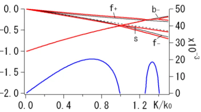
Fig. 1. Dispersion relation of parametric instabilities in the Hall-MHD system. Shown are the real (red lines, left scale) and imag-inary (blue lines, right scale) normalized frequencies plotted ver-sus the normalized wave number, K/ k0. Parameters used are,
k0=−0.5,β=0.5, andb0=0.4. For comparison, the dispersion re-lation of sideband wave modes and the sound wave (zero parent wave amplitude) is superposed as black solid and dashed lines, re-spectively. Forward and backward lower (upper) sideband waves are labeledf−(+)andb−(+), and the sound wave is labeleds.
where we write the subscripts(±1)as(±)for brevity. Com-bining these equations above, we obtain,
(2−βK2)L+L−=
K2b02
2 (L+R−+L−R+), (27) where
L±=ω±2 −k
2
±(1+ω±), (28)
R±=k0k±
k 0 ω0K
+ω±
k0K
−1−ω±
. (29)
The dispersion relation (27) has been obtained and solved numerically (Wong and Goldstein, 1986; Longtin and Son-nerup, 1986; Terasawa et al., 1986; Vinas and Goldstein, 1991; Hollweg, 1994; Champeaux et al., 1999). Figure 1 shows the real and imaginary frequencies of the longitu-dinal waves when β=0.5, b0=0.4, and k0=0.5. Under this particular set of parameters, the modulational instability (0<K/ k0<1) has a growth rate larger than (or almost com-parable with) the beat instability aroundk=1.3.
It is instructive to look at Eqs. (23) and (24) in order to discuss how the side band mode frequencies are determined. The r.h.s. of these equations represent three basic processes which determine the transverse magnetic field; the linear re-sponse (k±v±(∗)), the v×bnonlinearity (k±b0u1/2), and the Hall effect (k±2b
(∗)
± −b0k0k±ρ/2). Hereafter we will call
these terms as “linear”, “nonlinear”, and the “dispersive” terms, respectively. For a given set of parent wave param-eters (b0 andk0),β, andK, one can solve Eq. (27) to find associated with the modulational instability (eigenvalue), together with ratios among variables,ρ1,u1, b(±∗), andv
(∗)
±
Fig. 2. The three frequency contributions,ωlin,ωnl, andωdisp, plotted versusk, using the same set of parameters used for Fig. 1. See text for explanation of how to make the plot. Both Re[ω] (red solid line) andωlinare linearly dependent onk, and so should be the sum ofωdispand ωnl, suggesting that the dispersion and the nonlinear effects are cancelled each other.
(eigenvector). By varyingK in both positive and negative regimes, the dispersion relation can be visualized by plot-ting the real part ofω≡ω0+as a function ofk≡k0+K, as shown in Fig. 2 as a solid red line. Superposed in the figure are the plots ofωlin=(k±v(±∗))/b
(∗)
± ,ωnl=k±b0u1/2b(±∗), and
ωdisp=k±2−b0k0k±ρ/2b(±∗) versus k, which are frequency
contribution from the three effects introduced above. By def-inition,ω=ωlin+ωnl+ωdisp.
From the figure we notice that bothωandωlinalmost
lin-early depend onk, and thus sum ofωnl andωdispshould also depend linearly onk, suggesting that the nonlinear effect and the dispersion effect are balanced, as they were for the DNLS equation discussed previously. In other words, the mismatch of the resonance condition due to the dispersion effect is re-duced by nonlinear interaction among the Fourier modes, just like in the case of the DNLS (Sect. 2.1).
3 Phase coherence in the DNLS equation
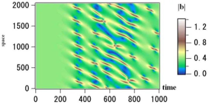
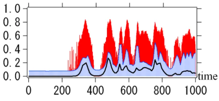
Fig. 3.Time evolution of envelope|b|in the DNLS model (11) with periodic boundary conditions. Initial conditions are given as a su-perposition of finite amplitude, left-hand polarized monochromatic waves, and very small amplitude white noise.
very small amplitude white noise with<|bnoise|2>1/2=10−5 within the range of −256<m<256, where the bracket de-notes spatial average over the simulation system. In the above, the wave numberkis related to the mode numberm as k=2π m/L, where the system size isL=256. We have used the convention thatmandkpositive (negative) repre-sents the right- (left-) hand polarized waves. For the numeri-cal computation, we have employed the rationalized Runge-Kutta scheme for time integration and the spectral method for evaluating spatial derivatives. Number of grid points used for this run is 2048.
Since in Fig. 3 we are plotting the magnetic field enve-lope, which is constant for the monochromatic, circularly polarized waves, at the beginning not much wave activities are apparent. However, starting fromt∼200, modulation of the envelope becomes increasingly more evident, and around t∼300 a series of solitary waves is created. The number of solitary waves is decided by the wave number that has the largest growth rate in Eq. (13). Aftert∼300 we observe a complex behavior of solitary waves: they appear, propagate, disappear, and interact with each other.
Corresponding time evolution of the power spectrum is shown in Fig. 4. During 0<t.200, the parent wave energy (m=−11) is gradually transferred to the side-band daughter waves (mainly, m=−4 and m=−18) through the modula-tional instability. Later on, increasingly more waves at dif-ferent mode numbers are generated due to coupling among finite amplitude waves, and also due to the modulational in-stability of the daughter waves, as can be seen as widening of the power spectrum in them-space. Aroundt∼300, the width of the spectrum is maximized, corresponding to the appearance of the solitary waves. When the solitary waves disappear, the power spectrum becomes narrow again, repre-senting the uncertainty principle, i.e., the width of the wave packet in the real and Fourier space are inversely proportional to each other. We note that solitary waves disappear almost completely at certain time intervals liket∼900. This is
remi-Fig. 4.Time evolution of the power spectrum (in logarithmic scale), log|bm|, plotted in the phase space of the wave mode number (m) and time. The parent mode is given initially atm0=−11. Positive (negative)mcorresponds to right- (left-) hand polarized waves. The wave number is given byk=2π m/L, whereL=256 is the system size.
niscent of the presence of (near) recursion of the DNLS equa-tion with periodic boundary condiequa-tions.
Next we show that distribution of wave phases and fre-quencies are closely related to the generation and disappear-ance of the solitary waves. We write the Fourier transformed magnetic fieldbk=|bk|expiφk, and discuss the relation
be-tween behavior of solitary waves and correlation among wave phases,φk. A method to evaluate the wave phase
coher-ence has been proposed (Hada et al., 2003; Koga and Hada, 2003), which we briefly explain below: Suppose we have a data containing waves, BORG(x), where “ORG” stands for “original data”. In the present analysis, this is a snapshot of simulation data evaluated at certain fixed time. From BORG(x) we make a phase randomized surrogate (PRS), BPRS(x), and a phase correlated surrogate (PCS),BPCS(x), by shuffling and making equal all the phases, respectively. Then we compute the “phase coherence index”,
Cφ=(LPRS−LORG)/(LPRS−LPCS), (30) where
L∗=
X
x
|B∗(x+δ)−B∗(x)| (31)
is the first order structure function evaluated for data (*), and the asterisk stands for either ORG, PRS, or PCS. In the above,δ is an external parameter representing the coarsing scale, which we choose to be the grid size for the present analysis. WhenCφis close to 0, wave phases are almost
ran-dom, whileCφbeing close to unity suggests that phases are
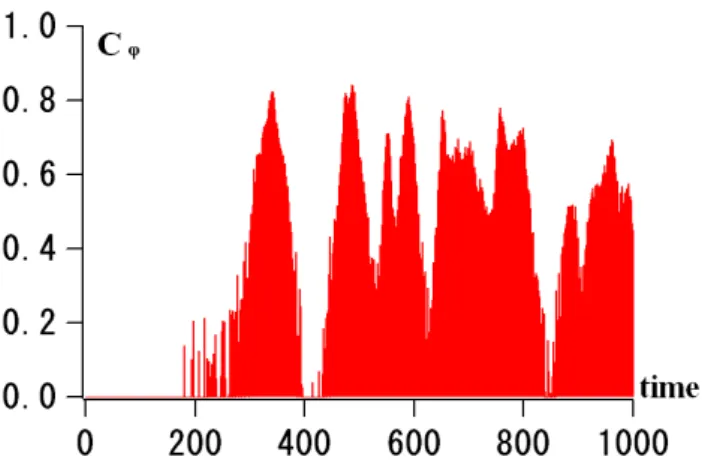
almost completely coherent. Figure 5 shows time evolution ofCφfor the run shown in Fig. 3. Apparently, the
appear-ance and disappearappear-ance of solitary wave trains correspond to the increase and decrease ofCφ. This is easily understood
Fig. 5. Time evolution of the phase coherence index,Cφ. When
Cφ∼0, the wave phases are almost random, whileCφ∼1 represents that the wave phases are almost completely correlated.
Now we discuss how phase coherence is generated by the modulational instability in the DNLS. Since the nonlinearity of the DNLS equation is cubic, it follows that, the basic non-linear interaction in this model is the four wave resonance. (On the other hand, if we regard|b|2as a quasi-mode as rep-resented in the static approximation (10), the interaction can be viewed as the three wave resonance among two Alfv´en waves and the quasi-mode.)
We have the resonance relation among the wave numbers,
k1+k2=k3+k4, (32)
and a similar relation should hold for the wave frequencies as well. While the resonance condition of the wave frequen-cies usually has the mismatch due to the dispersion effect in the DNLS, as we saw in Sect. 2, the dispersion effect and the nonlinear effect cancels each other, and so there is no mis-match of frequencies when the wave modes are coupled.
Let us define the relative phase among the four waves as θ (k)≡φk1+φk2−φk3−φk4, (33) where k={k1, k2, k3, k4} represents the quartets of wave modes in resonance. Small temporal change ofθ (k)implies that the phase coherence between the four waves is strong (locked), because this temporal change corresponds to the mismatch of the resonance condition of frequencies.
From Eqs. (11) and (33), we have d
dt
|bk1|2 2
! =k1
X
|bk1||bk2||bk3||bk4|sinθ (k), (34) and
d
dt(φk1)=k1
X|bk2||bk3||bk4| |bk1|
cosθ (k)+k12, (35) where the summation is to be taken over all the combinations of(k2, k3, k4)which satisfy (32). Equation (34) indicates that
F
k
|d
θ/
dt|
Fig. 6.Relation betweenF (k)and| ˙θ (k)|(see text for detailed ex-planation of the plot and the variables). The set of wave numbers chosen for the plot arekj=2π mj/L, whereL=256 is the system size, andm3=m4=m0=−11,m1=−15, m2=m3+m4−m1=−7. The figure suggests that the exchange of wave energy between the sites is enhanced (reduced) when the relative phase is almost con-stant (varies rapidly) in time. The unit of the vertical axis is degrees per unit time.
the evolution of wave energy of a certain mode is determined by “energy flow” exchanged between the quartets,
F (k)≡k1|bk1||bk2||bk3||bk4|sinθ (k). (36) The direction of the energy flow is determined by the sign of sinθ (k)andk1.
Figure 6 is a scatter plot in the phase space ofF (k)and
coherence (Fig. 5), since a large number of quartes undergo significant nonlinear interaction among them as evidenced in Fig. 6.
The interpretation above is justified by inspection of the dispersion relation directly computed from the simulation run. By computingφ˙k using (35) and plotting it versusk1, the dispersion relation in the simulation system can be visu-alized for any given time. In Fig. 7 we show time evolution of the dispersion relation, att=0,t=200, andt=550. Initially, almost all the wave modes have extremely small amplitude except for the parent wave, and thus they are located around the linear dispersion relation,ω=b20k+k2. As many of the wave modes acquire finite wave amplitude via the wave-wave interaction, they tend to be aligned on straight lines (two line segments exist in (b): notice a little difference in slopes of lines forkpositive and negative). The slope of the line cor-responds to the propagation speed of a soliton, and the in-terval ofkwhich are aligned on the line segment represent the waves the soliton is composed of. At later time (c), it is more evident that the wave modes are concentrated on a number of different line segments, with different ranges ofk, and with different slopes. These line segments do not nec-essarily go through the origin, since they represent the four (but not three) wave interaction. Consequently, even though there can be many solitary waves (coherent structures) with different propagation speeds, the resonance condition among the four waves is well satisfied, i.e., the frequency mismatch is small, and thus a large flow of energy exchange among the modes is expected.
The nonlinear interaction among different waves can be inspected through evaluation of the so-called bi-coherence (Dudok de Wit et al., 1999; Diamond et al., 2000),
bc(k1, k2, k3)=
|< ρk1bk2bk∗3>| p
<|ρk1bk2|2><|bk3|2>
. (37)
Presence of finite wave power at k1, k2, k3, together with bc∼1 suggests that the waves are in resonance. Figure 8 compares time evolution of averaged bi-coherence index, bφ=N−1Pbc, total absolute energy flow among all the
quartets, Ftot=N−1P|F (k)|, and the phase coherence in-dex,Cφ. On computingbφandFtot, all the combinations of wave numbers (Ndifferent ways) are exhausted. Apparently variations of the three quantities agree well to each other, suggesting that the phase coherence is generated as the wave energy is exchanged among resonant quartets.
Finally, we make a remark on the direction of the en-ergy flow. From Fig. 4 we see that the parent wave mode (k=k0=2π m0/L) remains to be the dominant one throughout the simulation run. Therefore, among the many quartets of wave modes in resonance (k1, k2, k3, k4) with k1+k2=k3+k4, the most dominant quartet (which makes (36) the largest) is the one withk3=k4=k0. The resonance condition of wave number for this quartet is,
k0+k0=k1+k2. (38)
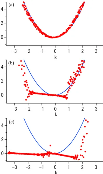
Fig. 7. The wave frequencyφ˙k(red circles) versuskevaluated at (a)t=0, (b)t=350, and (c)t=550. Att=0, all the wave modes ex-cept for the parent wave have very small wave amplitude, and thus they are located around the linear dispersion relation,ω=b20k+k2
(blue line). However, as the wave modes grow via wave-wave inter-action, they tend to be aligned along straight lines. The slope of the line corresponds to the propagation speed of a soliton, and the inter-val of k which are aligned on the line segment represent the waves the soliton is composed of. Among the quartet of waves on a sin-gle line, the frequency mismatch for the resonance condition| ˙θ (k)| is small, and consequently, energy exchange among themF (k)is large, as seen in Fig. 6.
Fig. 8. Time evolution ofCφ (red area), bφ (blue area), and
Ftot/10−6, (black solid line). Variation ofCφwell corresponds to those ofbφandFtot.
Fig. 9.Evolution of sinθ (k), plotted in the phase space of the wave mode number (m1) and time.
solitary wave rows (t∼200−350), sinθ (k)<0 fork1<0 and sinθ (k)>0 fork1>0. Namely, in both regimes ofk1>0 and k1<0, the energy flow defined in Eq. (36) is positive, i.e., the energy is transferred from the parent wave to the daughter waves. During the time interval when solitary waves disap-pear (t∼350−400), we observe the opposite, i.e., the energy flows back from the daughter to the parent waves.
4 Nonlinear relation among phase and frequency: Hall-MHD equations
In this section, we discuss the modulational instability in the Hall-MHD equations (Eqs. 5–8), and compare the results with that in the DNLS.
Numerical time integration of the Hall-MHD set of equa-tions, Eqs. (5–8), is performed, in a similar way as for the DNLS equation discussed in the preceding section. As initial conditions, finite amplitude, left-hand polarized, monochro-matic, parallel Alfv´en waves are given, with the wave am-plitudeb0=0.4 and the mode numberm=m0=−20. Super-posed with the parent wave is a small amplitude white noise
Fig. 10.Time evolution of envelope|b|due to Eqs. (5–8) with peri-odic boudary conditions. Initial conditions are given as a superposi-tion of finite amplitude, left-hand polarized monochromatic waves, and very small amplitude white noise.
with<|anoise|2>1/2=10−5, wherearepresents any variable in Eqs. (5–8) within the range of−128<m<128. The sys-tem size isL=256, in which there are 1024 grid points. We choseβ=0.5 so that the modulational instability growth rate is the largest among all the parametric instabilities possibly driven unstable. The parameters specified here are essen-tially equivalent to the ones used in the previous section.
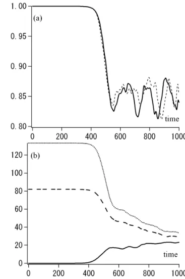
Figure 10 shows time evolution of|b|plotted in a way sim-ilar to Fig. 3, and Fig. 11 represent time evolution of log|bm|
and log|ρm|, which is the power of the transverse and the
longitudinal waves, respectively, as a function of the wave mode number,m.
From comparison of the DNLS and the Hall-MHD simu-lation runs, we dicuss validity of various approximations as-sumed in the DNLS. In particular, we look at the following: (a) the quasi-static approximation, Eq. (10), (b) conservation of the magnetic field energy alone, and (c) the assumption of constant plasma density in the dispersion term (i.e., the Hall-term,∂/∂x(ρ−1∂b/∂x), is simplified by assumingρto be constant). These approximations are justified as long as the power of the longitudinal modes (Fig. 11b) is much less than that of the transverse modes (Fig. 11a). Aroundt∼350, the power spectrum of sideband wave modes and the daugh-ter wave modes begin to grow. To check the validity of the approximation in Eq. (10), we evaluate the cross-correlation function,
c(λ, τ )= <|b(x+λ, t+τ )|
2ρ(x, t ) > p
Fig. 11. Time evolution of power spectrum (in logarithmic scale), log|bm| and log|ρm|, plotted in the phase space of the wave mode number (m) and time. The parent mode is given initially at
m0=−20. Positive (negative)mcorresponds to positive (negative) helicity.
energy both decrease. Aroundt∼500, inverse cascade begins to take place (discussion of the inverse cascade in the DNLS can be found in Krishan and Nocera, 2003).
The validity of the static approximation has been exam-ined by several authors. By performing hybrid (kinetic ions + an electron fluid) simulations, Machida et al. (1987) ar-gues that the system automatically adjusts itself to a state described by the static approximation when ion kinetic ef-fects are included. However, as time elapses, longitudinal mode grows and the static approximation is soon violated. Spangler (1987) concluded that the breakdown of the static approximation takes place in association with rapid evolu-tion of wave packets by ponderomotive force. Combining
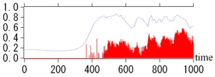
Fig. 12. Time evolution of(a)the cross-correlation,c(λ=0, τ=0)
evaluated for the run shown in Fig. 10 (solid line), andc(0,0) eval-uated for a run in which the advection term is artificially removed from the Hall-MHD set of equations (broken line). (b)magnetic field energy (broken), perpendicular kinetic energy (dotted), and parallel kinetic energy (solid), plotted versus time. Aroundt∼350, together with the decay of the cross-correlation function, the mag-netic field and the perpendicular kimag-netic energy decrease and the parallel kinetic energy increases.
Eqs. (5) and (6), we have ∂2ρ
∂t2 −β ∂2ρ ∂x2 =
∂2 ∂x2
|b|2
2 +ρu 2
. (40)
This equation describes propagation of sound waves in a presence of a source term (r.h.s.), which consists of the ponderomotive force, |b|2/2, and the advection effect, ρu2 (Spangler, 1987). The latter represents the “self-coupling” of longitudinal waves.
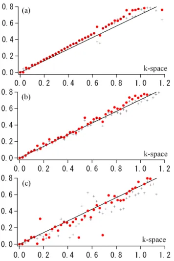
Fig. 13. Numerically obtained dispersion relation at(a)t=350,(b) t=500,(c)t=720. The blue line indicates the linear dispersion re-lation, and the red circles and black crosses show the frequency evaluated from the temporal variation of the magnetic field mode (φ˙kb) and that of the density modes (φ˙kρ), respectively. Superposed (green) line has a slope equal to the phase velocity of the wave mode which has the maximum power. Corresponding to the appearance of solitary waves and localized structures, the wave power tends to be aligned along a straight line.
are artificially removed from the Hall-MHD set of equations. The broken line in Fig. 12a depicts time evolution of the cross correlation function evaluated for the run without the advection terms, using the same simulation parameters as the previous run. The time evolution for both runs are es-sentially the same, suggesting that the process playing the most dominant role in violating the static approximation is the ponderomotive force, as suggested by Spangler (1987). The self-coupling term cannot be neglected, however, since its magnitude becomes comparable to other terms as the lon-gitudinal wave modes grow.
In a similar way described before to plot the dispersion re-lation of nonlinear Alfv´en waves in the DNLS directly from the simulation run, we have computed theφ˙kρ andφ˙kb, using Eqs. (5) and (8), respectively. Corresponding to appearance of solitary waves and localized structures, the frequency dis-tribution (φ˙kρ andφ˙bk), i.e., the dispersion relation, appears along a straight line, as shown in numerically evaluated dis-persion relation, Fig. 13. Since these waves propagate in the same direction as the parent wave, the frequency distribution along a straight line is usually satisfied at the origin. Fur-thermore, Fig. 13 shows that the longitudinal and transverse wave modes have a similar slope, which is the velocity of the structures composed of these waves. Thus, the three wave resonance condition between the transverse wave modes and the longitudinal wave modes is approximately satisified.
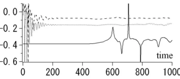
Figure 14 displays time evolution of the wave frequency (φ˙bk) for the parent wave (m=−20, solid line), and some of the daughter waves (m=−8, dotted line) (m=−3, broken line). When 0<t <∼500, the parent wave mode is dominant, and its frequency stays almost constant. Aroundt∼500, the inverse cascade begins to take place, and the parent wave frequency starts to be modified. On the other hand, the fre-quencies of the lower sideband wave modes remain almost constant (broken line). Thus, the phase velocity of the modes with the maximum power is close to the velocity of the struc-tures, and it corresponds to the slope of the dispersion rela-tion in Fig. 13.
Now we examine the approximation (c) we listed before in the DNLS, i.e., the assumption of constant density in the Hall term. In order to do so, let us explicitly write down the phase relation of Eq. (8),
dφkb
dt =ωnl+ωdisp+ωlin, (41)
ωnl =k X
k=k1+k2
|uk1||bk2| |bk|
cos(θkbub=k1+k2), (42)
ωdisp=k3k X
k=k3+k4
|bk3||Vk4| |bk|
cos(θkbbV=k3+k4), (43)
ωlin= −k |vk| |bk|
cos(φkb−φvk), (44)
whereV=ρ−1andθkxyz=l+m=φkx−φly−φmz. In the linear per-turbation analysis in Sect. 2.2 we have calledωnl,ωdisp, and ωlin as contribution to the wave frequency via “nonlinear”, “dispersion”, and “linear” effects, respectively. The disper-sion effect is not simplyk2, but isk2−b0k0Kρ/2/b±(∗), where
the latter term arises due to longitudinal perturbation. Just like in the DNLS model, the balance between the “nonlin-ear” and the “dispersion” terms also exist in the Hall-MHD equations.
Fig. 14. Time evolution of the wave frequency (φ˙kb) for the waves withm=−20 (solid line),m=−8 (dotted line), andm=−3 (bro-ken line). The wave number of these modes arek=−0.49,−0.19, and−0.07, respectively. When 0<t.500, the parent wave mode is dominant, and its frequency is almost constant. Aroundt∼500, the inverse cascade begins to take place, and the parent wave frequency starts to vary. On the other hand, the frequencies of the lower side-band wave modes remain almost constant aftert >500.
regarded as self-generation of the (dispersive) Walen’s rela-tion, which is the relation between the transverse magnetic and the velocity field satisfied for Alfv´enic fluctuations and rotational discontinuities (e.g., Landau and Lifshitz, 1962). For example, the normalized magnetic and the velocity field, b0andv0in Eqs. (14–15), satisfyv0= ∓b0/vφ0, where the signs represent parallel/anti-parallel propagation with respect to the background magnetic field, and the phase velocityvφ0 is determined from the dispersion relation (16). The term cos(φkb−φvk)in the r.h.s. of Eq. (44) takes the value of ei-ther 1 or−1 (so thatωlin/ k=±|vk|/|bk|) in association with
broadening of the power spectrum. Also, from Figs. 13 and 15, we find numerically thatωlin/ k∼k/ω (corresponding to the appearance of near straight lines in these plots). There-fore we find that the system approaches automatically to a state wherek/ω= ± |vk|/|bk|(Walen’s relation) is
automat-ically fulfilled. Furthermore, sinceωlinis almost linear ink in Fig. 13, so is the sum ofωdisp andωnl as Eq. (41)
sug-gests, i.e., the contribution to the wave frequency nonlinear inkis cancelled due to balance between the dispersion and the nonlinear effects.
Figure 16 shows distribution ofφ˙uk (similar toφ˙kρ) versus k. When 0<t.500, these longitudinal fluctuations are found to be distributed along the same straight line in the disper-sion relation, and should be recognized as the ponderomo-tive density fluctuations, produced via interaction of Alfv´en waves. In the present case, the fluctuations are produced in the course of the modulational instability, and the two in-teracting Alfv´en waves are on the same branch with nearly equal wave numbers and the wave frequencies, so that the resultant ponderomotive fluctuations have similar phase ve-locity as the interacting Alfv´en waves. The phase velocities of the longitudinal fluctuations (ρ anduin Fig. 16), trans-verse fluctuations (bandvin Fig. 13), and the acoustic wave (solid line in Fig. 13), are measured as∼0.78,∼0.78, and
Fig. 15. The three basic elements of the wave frequency,ωlin(light blue squares),ωnl(blue circles), andωdisp(green crosses), defined in Eqs. (42–44), plotted versusk, evaluated at(a)t=350,(b)t=500, and(c)t=720. As discussed in Sect. 2.2,ωlinis almost linear in
k, suggesting that the dispersive Walen’s relation is held. Since the dispersion relation (Fig. 13) suggests that the wave frequency, which is a sum of the three terms above, is linear ink also, the linearity inkof the sum ofωdispandωnl should be held as well, indicating that the dispersion and the nonlinear effects cancel each other, and the system is brought to a state where the wave resonance condition is easily satisfied.
Fig. 16. Numerically computed frequencyφ˙uk(red circles) andφ˙kρ
(black crosses) versus the wave numberkat(a)t=350,(b)t=500, (c)t=720. When 0<t.500, the longitudinal modesφ˙u
k,φ˙ ρ k are dis-tributed around a line slightly (but distinctly) above the sound wave branch (solid black line). The former may be called the “pondero-motive density fluctuation” branch. As later times, however, we find that the longitudinal wave frequencies are re-distributed around the sound branch.
fluctuation acts as a driver to excite the sound waves, as rep-resented in Eq. (40).
This excitation of the sound wave is also related to particle heating due to the modulational instability of Alfv´en waves. Many authors discussed Landau damping associated with en-velope modulation of Alfv´en waves (Mjølhus and Wyller, 1986, 1988; Spangler; 1989, 1990; Medvedev and Diamond, 1996; Passot and Sulem; 2003). However, the ion acoustic wave mode is exclueded, as long as the “ponderomotive” ex-pansion is used in scaling of the system. In the case of the weak nonlinearity, the “triple-degenerate” expansion makes a similar description atβ∼1 (Hada, 1993). The kinetic ”triple-degenerate” DNLS equation will be useful for elucidating the physics of the heating process. The use of numerical
simula-tion models (Vasquez, 1995) and/or theoretical models (Sny-der, 1997; Passot and Sulem, 2004) that include the strong nonlinearity and kinetic effects are desired.
5 Conclusions and discussions
In this paper, we discussed the nonlinear relation among phases and frequencies in the modulational instability of parallel propagating Alfv´en waves in the context of one-dimensional two fluid models, using linear perturbation anal-ysis and numerical experiments.
The main results of the present paper may be summarized as follows:
(1) Corresponding to generation of solitary waves or co-herent structures by the wave modulation, dispersion relation of the waves tend to be aligned along straight segments of lines (Figs. 7 and 13). The slopes of these straight lines cor-respond to velocities of the solitary waves and the structures, and are well estimated as the phase (∼the group) velocity of the wave with the largest wave power.
(2) The exchange of wave energy among the resonant wave modes is enhanced (reduced) when the relative phase is close to constant (varies rapidly) in time (Fig. 6). This is a universal feature in a wide variety of nonlinear systems: e.g., it can also be seen in a single triplet model (Appendix A).
(3) The fact that the dispersion relation is essentially given as segments of lines in the dispersion relation suggests that the mismatch in the resonance conditions among the coupled wave modes is reduced automatically. The waves can effi-ciently exchange wave energy and generate the phase coher-ence.
In the DNLS equation (Sect. 3), increase and decrease of the phase coherence index well corresponds to the appear-ance and disappearappear-ance of solitary wave trains. However, in the Hall-MHD equations (Sect. 4), evolution of the phase co-herence index turns out to be more complex. There are two issues to be discussed: the physical processes leading to the variation of the phase coherence index, and the validity of the index.
In the DNLS, the energy flow among the wave modes gen-erates order not only among the wave frequencies but also among wave phases (see Appendix A, and also Fig. 9), and the associated broadening of the power spectrum always cor-responds to the global energy flow because of the balance between the dispersion effect and the nonlinear effect. How-ever, in the Hall-MHD, the presence of the localized struc-tures does not always correspond to the broadening of the power spectrum. In Fig. 17 we plot time evolution ofCφ
andbφbased on the Hall-MHD simulation run discussed
be-fore. The broadening of the power spectrum correlates well withbφ, but not quite well withCφ. This probably is due to
Fig. 17. Time evolution ofCφ(red area) andbφ(broken line). In association with the broadening of the power spectrum,bφvaries accordingly, butCφdoes not.
In case of the modulational instability starting from a sin-gle parent wave plus small amplitude background noise, one can evaluate the relative phase among the resonant wave modes and also the energy flow among them, and identify clearly time intervals the phase coherence is generated (see Fig. 9, and also early part of Fig. 18). On the other hand, after the initial stage of the modulational instability, wave modes at low wave numbers produced via the inverse cascade be-come dominant, it is no longer possible to identify the time intervals in which the phase coherence is produced.
Regarding the phase coherence index, we have to say that its physical meaning is still not completely clear, although it was demonstrated that the index is a useful measure to iden-tify the presence of wave-wave interaction (Koga and Hada, 2003). Since the concept of the phase synchronization is uni-versal (e.g., He and Chian, 2005), it is important to develop a method that can characterize the underlying nonlinearity of the system. This discussion is translated into the explanation or improvement of the phase coherence index.
The relation between the longitudinal and transverse modes has important information on the nature of the para-metric instability. In the dispersion relation, longitudinal and transverse modes were found to be both linear, with almost the same slope, corresponding to the structures generated by modulational instability. On the other hand, the longitudi-nal fluctuations generated by the decay instability distribute on the sound wave line with some band width (Terasawa et al., 1986). Such a cross relation among different variables in MHD turbulence is very important to understand the turbu-lent dynamics. Henceforth, we have to analyze in detail the general rules of the relation among these variables in parallel Alfv´en turbulence generated by parametric instability. Also, it is essential to include the kinetic effects whenβis moder-ately large.
It is important to identify the phase coherence brought by nonlinear wave-wave interaction, in order to discuss under-lying physical processes leading to the generation of the co-herent structures. This is particularly important for analysis of spacecraft data, since there are many localized structures in space plasmas which are produced, presumably, by pro-cesses other than nonlinear wave-wave interactions. Dudok
Fig. 18. Time evolution of the relative phase between the parent and the other wave modes, sin(φkb0−φkb1−φuK).
de Wit et al. (1999) and Soucek et al. (2003) discussed the so-called Volterra model, a way to identify nonlinear wave-wave interactions using the satellite and the simulation data, by utilizing the high order spectrum analyses and weak tur-bulence theory. This method may shed light on understand-ing the nature of wave-wave interactions when the weak and strong turbulence processes co-exist. In the future, we hope to clarify the process of the phase coherence generation via the wave-wave interaction in more detail, and to extend the Volterra-type models in such a way that the weak turbulence approximation is not necessary.
Finally, we make a remark on energetic particle transport in the turbulence including the localized structures. Since these structures have broad power spectrum in thekspace, particles with wide range of energy can resonate with them. However, this is not the more important side of the wave-particle interaction, from the viewpoint of the phase coher-ence – rather, it is in the fact that large amount of electro-magnetic field and plasma energy is concentrated within the solitary wave (phase correlated wave/structure), so that it can influence particle motion via strong and correlated impulse force rather than via sequence of random forces which last for a long time.
Fig. A1. Time evolution of Nj with the initial condition,
N3≫N1, N2. The broken, dotted, and solid lines indicateN1,N2, andN3, respectively. The system is “unstable” in that the “quanta” originally stored in mode 3 are re-distributed to modes 1 and 2 within an instability time scale (∼3000).
dominance between the ballistic and trapped trajectories, en-semble of these particles may appear as either super- or sub-diffusive (Zimbardo et al., 2000; Carreras et al., 2001). In order to properly describe time evolution of the ensemble, one has to invoke the fractal diffusion formalism (Metzler and Nonnenmacher, 1998; del-Castillo-Negrete et al., 2004).
Appendix A
Three wave resonance: a single triplet
A triplet is known as the most basic element of nonlinear interaction that can be extracted from various phenomena. Decay instability of Alfv´en waves in space plasma is an ex-ample. A finite amplitude Alfv´en wave propagating parallel to the ambient magnetic field decays into a backward prop-agating Alfv´en wave and a forward propprop-agating ion acoustic wave. We consider a set of three wave equations (3W) dis-cussed by Sagdeev and Galeev (1969),
˙
C1= −iC2∗C3, (A1)
˙
C2= −iC1∗C3, (A2)
˙
C3= −iC1C2, (A3)
whereCj is the normalized complex amplitude of thej-th
mode. The above set of equations is derived via resonance condition among frequencies of each mode,
ω3=ω1+ω2. (A4)
By introducing the wave quanta (wave action), Nj=|Cj|2=ǫj/ωj, where ǫj is the wave energy of
modej, we have the Manley-Rowe relations,
N1+N3=const, (A5)
Fig. A2. Same as Fig. A1 except that the initial condition here isN2≫N1, N3. The broken, dotted, and solid lines indicateN1,
N2, andN3, respectively. The system is “stable” in the sense that variations ofN1,N2, andN3are small.
N1−N2=const. (A6)
Now let us writeCj=Ajexp(iφj), withAj(=pNj)andφj
real, then we obtain a relation about the phase difference among the triplets (θ=φ3−φ2−φ1),
˙
θ= ˙φ3− ˙φ2− ˙φ1, (A7)
= −(A1A2 A3
−A2A3
A1
−A3A1
A2
)cosθ, (A8)
=cotθ d
dtlog(A1A2A3), (A9)
where φ˙j is the (nonlinear) frequency andθ˙ represents the
frequency mismatch in the resonance condition. From the above, the following conservation law is derived
A1A2A3cosθ=D0=const. (A10) The 3W equations at a glance have six degrees of freedom, but if we write them into the real amplitude and phase, we find that the equations actually have only four degrees of freedom: the real amplitudesA1,A2,A3, and the phase dif-ferenceθ. Since there are three invariants (A5, A6, A10), the 3W equation set is integrable. All initial problem of 3W can be solved, and the solution can be written using elliptic func-tions. Behavior of the system may be physically interpreted as either stable or unstable depending on initial distribution of wave quanta to the three eigenmodes (Figs. A1 and A2).
Let us define the flow of quantaF, which represents the interaction between the eigenmodes,
F = ˙N1= ˙N2= − ˙N3=2A3A2A1sinθ, (A11) and consider its relationship to temporal change of the phase differenceθ. The sign of sin˙ θ determines the direction of quanta flow.
Fig. A3. Time evolution ofN1,N2,N3, andθ for the case that
A1A2A3cosθ=0.
quanta, and the second is that all the modes have some finite number of quanta. In the first case, cosθ=0 always since D0=0. In Fig. A3, we see thatθ jumps 180 degrees peri-odically because the direction of the quanta flow remain un-changed per half the oscillation period.
From now on, we only discuss the case where all the modes have some finite number of quanta. Since D0=const6=0, we can rewriteF as
F =2D0tanθ, (A12)
and therefore, the condition−π/2<θ <π/2 is required in or-der thatF be finite. This condition is evident from Eq. (A10). Equation (A12) suggests that|F|is large whenθis close to either−π/2 orπ/2, whileF=0 whenθ=0 (Fig. A4a).
Figure A4b shows time evolution of φ˙j. Both fast and
slow temporal changes ofθ can be seen. Around the point where the number quanta is close to take extremal values, the temporal change ofθ becomes rapid. If the system is unstable, temporal change of the phase difference is much faster when the quanta is at local minimum, than when it is at local maximum. Figure A4c shows this relationship more clearly. Using Eqs. (A10) and (A12), andφ˙j=−D0/Nj, we
have
˙
θ= −D0( 1 N3
− 1
N1
− 1
N2 )=D0
˙
F
2G2, (A13)
where G=A1A2A3. This equation exactly shows the rela-tionship discussed above.
In summary, if the temporal change of the phase differ-ence is small (large), quanta flow between the modes is large (small). In other words, the stronger (weaker) the modes are correlated, are the interaction between the modes strong (weak). This relationship between the phase coherence and the interaction among eigenmodes is universal. For example, similar relationship is held in a system where many triplets are connected, in the DNLS, and in the Hall-MHD models. Also, when cosθ=0 initially, we have a situation similar to the case thatNj=0 for one (or more) of the modes, and thus
cosθ=0 always.
Fig. A4. (a)The energy flowF(solid line, left axis) and sinθ (dot-ted line, right axis) are plot(dot-ted versus time. When the energy is exchanged between the modes, the relative phase stays at almost at a constant level. The same tendency is observed in systems with multiple degrees of freedom (cf., Figs. 9 and 18). (b)Time evolu-tion ofφ˙j. The thin, solid, and dotted lines indicateφ˙1,φ˙2, and
˙
φ3, respectively.(c)Relation betweenθ˙andFfor a (single) triplet. The exchange of quanta between the sites is enhanced when the rel-ative phase is approximately constant in time, while the exchange of quanta is reduced when the relative phase varies rapidly.
Acknowledgements. We thank S. Matsukiyo and D. Koga for fruitful discussions and valuable comments. This paper has been supported by JSPS Research Felowships for Young Scientists in Japan.
References
del-Castillo-Negrete, D., Carreras, B. A., and Lynch, V. E.: Frac-tional diffusion in plasma turbulence, Phys. Plasmas, 11(8), 3854–3864, 2004.
Carreras, B. A., Lynch, V, E., and Zaslavsky, G. M.: Anomalous diffusion and exit time distribution of particle tracers in plasma turbulence model, Phys. Plasmas, 8(12), 5096–5103, 2001. Chanpeaux, S., Laveder, D., Passot, T., and Sulem, P. L. : Remarks
on the parallel propagation of small-amplitude dispersive Alfv´en waves, Nonlin. Processes Geophys., 6, 169–178, 1999,
http://www.nonlin-processes-geophys.net/6/169/1999/.
Chen, X. J. and Lam, W. K.: Inverse scattaring transform for the derivative nonlinear Schr¨odinger equations with nonvanishing boundary conditions, Phys. Rev. E, 69, 066604, doi:10,1103, 2004.
Derby, N. F.: Modulational instability of finite-amplitude, circulary polarized Alfv´en waves, Astrophys. J., 224(3), 1013–1016, 1978. Diamond, P. H., Rosenbluth, M. N., Sanchez, E., Hidalgo, C., Van Milligen, B., Estrada, T., Branas, B., Hirsch, M., Hartfuss, H. J., and Carreras, B. A.: In seach of the elusive zonal flow using cross-bicoherence analysis, Phys. Rev. Lett., 84(21), 4842–4845, 2000.
Dudok de Wit, T., Krasnosel’skikh, V. V., Dunlop, M., and Luhr, H.: Identifying nonlinear wave interactions in plasmas using two-point measurements: A case study of Short Large Amplitude Magnetic Structures (SLAMS), J. Geophys. Res., 104, 17 079– 17 090, 1999.
Galeev, A. A., Oraevskii, V. N., and Sagdeev, R. Z.: Universal in-stability of an inhomogeneous plasma in a magnetic feild, Sov. Phys. JETP, 17, 615–620, 1963.
Ghosh, S. and Papadopoulos, K.: The onset of Alfv´enic turbulence, Phys. Fluids, 30(5), 1371–1387, 1987.
Goldstein, M. L.: An instability of finite amplitude circularly polar-ized Alfv´en waves, Astrophys. J., 219(2), 700–704, 1978. Hada, T.: Evolution of large amplitude Alfv´en waves in the solar
wind withβ∼1, Geophys. Res. Lett., 20(22), 2415–2418, 1993. Hada, T., Koga, D., and Yamamoto, E.: Phase coherence of MHD
waves in the solar wind, Space Sci. Rev., 107(1–2), 463–466, 2003.
Hasegawa, A., Kodama, Y., and Watanabe, K.: Self-organization in Korteweg – de Vries turbulence, Phys. Rev. Lett., 47(21), 1525– 1529, 1981.
He, K. and Chian, A. C.-L.: Nonlinear dynamics of turbulent waves in fluids and plasmas, Nonlin. Processes Geophys., 12, 13–24, 2005,
http://www.nonlin-processes-geophys.net/12/13/2005/.
Hollweg, J. V.: Beat, modulational, and decay instabilities of a circularly polarized Alfv´en wave, J. Geophys. Res, 99, 23 431– 23 447, 1994.
Kaup, D. J. and Newell, A. C.: An exact solution for a derivative nonlinear Schr¨odinger equation, J. Math. Phys., 19, 798–801, 1978.
Kawata, T. and Inoue, H.: Exact solution of the derivative nonlinear Schr¨odinger equation under the nonvanishing conditions, J. Phys. Soc. Japan, 44, 1968–1976, 1978.
Kawata, T., Sakai, J.-I., and Kobayashi, N.: Inverse method for the mixed nonlinear Schr¨odinger equation and soliton solutions, J. Phys. Soc. Japan, 48, 1371–1379, 1980.
Koga, D. and Hada, T.: Phase coherence of foreshock MHD waves:
wavelet analysis, Space. Sci. Rev., 107, 495–498, 2003. Krishan, V. and Nocera, L.: Relaxed states of Alfv´enic turbulence,
Phys. Lett. A, 315, 389–394, 2003.
Kuramitsu, Y. and Hada, T.: Acceleration of charged particles by large amplitude MHD waves: effect of wave spatial correlation, Geophys. Res. Lett., 27(5), 629–632, 2000.
Landau, L. D. and Lifshitz, E. M.: Electrodynamics of continuous media, Pergamon, Oxford, New York, 1984.
Longtin, M. and Sonnerup, B.: Modulational instability of circulary polarized Alfv´en waves, J. Geophys. Res., 91, 798–801, 1986. Lucek, E. A., Horbury, T. S., Balogh, A., Dandouras, I., and
Reme, H.: Cluster obsevations of structures at quasi-parallel bow shocks, Ann. Geophys., 22, 2309–2314, 2004,
http://www.ann-geophys.net/22/2309/2004/.
Machida, S., Spangler, S. R., and Goertz, C. K.: Simulation of amplitude-modulated circularly polarized Alfv´en waves for beta less than one, J. Geophys. Res., 92(A7), 7413–7422, 1987. Mann, G., Luhr, H., and Baumjohann, W.: Statistical analysis of
short large-amplitude magnetic field structures in the vicinity of the quasi-parallel bow shock, J. Geophys. Res., 99(A7), 13 315– 13 323, 1994.
Medvedev, M. D. and Diamond, P. H.: Fluid models for kinetic effects on coherent nonlinear Alfv´en waves, Phys. Plasmas, 3(3), 863–873, 1996.
Medvedev, M. D., Diamond, P. H., Shevchenko, V. I., and Galinsky, V. L.: Dissipative dynamics of collisionless nonlinear Alfv´en wave trains, Phys. Rev. Lett., 78(26), 4934–4937, 1997. Metzler, R. and Nonnenmacher, T. F.: Fractional diffusion,
waiting-time distributions, and Cattaneo-type equations, Phys. Rev. E, 57(6), 6409–6414, 1998.
Mio, K., Ogino, T., Minami, K., and Takeda, S.: Modified nonlin-ear Schr¨odinger equation for Alfv´en waves propagating along the magnetic field in cold plasmas, J. Phys. Soc. Japan, 41, 265–271, 1976.
Mjølhus, E.: Application of the reductive perturbation method to long hydromagnetic waves parallel to the magnetic field in a cold plasma, Report no. 48, Department of applied mathematics, Univ. Bergen, Norway, 1974.
Mjølhus, E.: On the modulational instability of hydromagnetic waves parallel to the magnetic field, J. Plasma. Phys., 16, 321– 334, 1976.
Mjølhus, E. and Wyller, J.: Alfv´en solitons, Phys. Scr., 33, 442– 451, 1986.
Mjølhus, E. and Wyller, J.: Nonlinear Alfv´en waves in a finite beta plasma, J. Plasma Phys., 40, 299–318, 1988.
Mjølhus, E. and Hada, T.: Soliton theory of quasi-parallel Alfv´en waves, in: Nonlinear waves and chaos in space plasmas, edited by: Hada, T. and Matsumoto, H., Terrapub, Tokyo, 121–169, 1997.
Nariyuki, Y. and Hada, T.: Self-generation of phase coherence in parallel Alfv´en turbulence, Earth, Planets, Space, 57, e9–e12, 2005.
Nocera, L. and Buti, B.: Bifurcations of coherent states of the DNLS equation, Phys. Scr., T63, 186–189, 1996.
Passot, T. and Sulem, P. L.: Long-Alfv´en wave trains in collision-less plasmas. 1. Kinetic theory, Phys. Plasmas, 10(10), 3887– 3905, 2003.
5189,2004.
Rogister, A.: Parallel propagation of nonlinear low-frequency waves in high-beta plasma, Phys. Fluids, 14, 2733–2739, 1971. Sagdeev, R. Z. C. and Galeev, A. A.: Nonlinear Plasma Theory,
edited by: O’Neil, T. M., Book, D. L., and Benjamin, W. A., New York, 1969.
Sakai, J.-I. and Sonnerup, B.: Modulational instability of finite am-plitude dispersive Alfv´en waves, J. Geophys. Res., 88, 9069– 9078, 1983.
Snyder, P. B., Hammett, G. W., and Dorland, W.: Landau fluid models of collisionless magnetohydrodynamics, Phys. Plasmas, 4(11), 3974–3985, 1997.
Soucek, J., Dudok de Wit, T., Krasnoselskikh, V., and Volokitin, A.: Statical analysis of nonlinear wave interactions in simulated Langmuir turbulence data, Ann. Geophys., 21, 681–692, 2003, http://www.ann-geophys.net/21/681/2003/.
Spangler, S. R. and Sheerin, J. P.: Properties of Alfv´en solitons in a finite-beta plasma, J. Plasma Phys., 27, 193–198, 1982. Spangler, S. R.: The evolution of nonlinear Alfv´en waves subject to
growth and damping, Phys. Fluids, 29(8), 2535–2547, 1986. Spangler, S. R.: Density fluctuations induced by nonlinear Alfv´en
waves, Phys. Fluids, 30(4), 1104–1109, 1987.
Spangler, S. R.: Kinetic effects on Alfv´en-wave nonlinearity, 1. Ponderomotive density fluctuations, Phys. Fluids, B 1(8), 1738– 1746, 1989.
Spangler, S. R.: Kinetic effects on Alfv´en-wave nonlinearity, 2. The modified nonlinear-wave equation, Phys. Fluids, B 2(2), 407– 418, 1990.
Terasawa, T., Hoshino, M., Sakai, J.-I., and Hada, T.: Decay in-stability of finite-amplitude circulary polarized Alfv´en waves: A numerical simulation of stimulated brillouin scattering, J. Geo-phys. Res., 91, 4171–4187, 1986.
Tsurutani, B. T., Lakhina, G. S., Pickett, J. S., Guarnieri, F. L., Lin, N., and Goldstein, B. E.: Nonlinear Alfv´en waves, proton perpendicular acceleration, and magnetic holes/decreases in in-terplanetary space and the magnetosphere: intermediate shocks?, Nonlin. Processes Geophys., 12, 321–336, 2005,
http://www.nonlin-processes-geophys.net/12/321/2005/. Vasquez, B. J.: Simulation study of the role of ion kinetics in
low-frequency wave train evolution, J. Geophys. Res., 100(A2), 1779–1792, 1995.
Vinaz, A. F. and Goldstein, M. L.: Parametric instabilities of circu-larly polarized large-amplitude dispersive Alfv´en waves: excita-tion of parallel-propagating electromagnetic daughter waves, J. Plasma. Phys., 46, 107–127, 1991.
Wong, H. K. and Goldstein, M. L.: Parametric instabilities of circu-larly polarized Alfv´en waves including dispersion, J. Geophys. Res., 91, 5617–5628, 1986.