Nonlinear wave effects at the non-reflecting beach

www.nonlin-processes-geophys.net/19/1/2012/ doi:10.5194/npg-19-1-2012

© Author(s) 2012. CC Attribution 3.0 License.

Nonlinear Processes

in Geophysics

Nonlinear wave effects at the non-reflecting beach

I. Didenkulova1,2and E. Pelinovsky3,4

1_{Laboratory of Wave Engineering, Institute of Cybernetics at Tallinn University of Technology, Akadeemia tee 21,}

12618 Tallinn, Estonia

2_{Nizhny Novgorod State Technical University, Nizhny Novgorod, Russia}

3_{Department of Nonlinear Geophysical Processes, Institute of Applied Physics, Nizhny Novgorod, Russia} 4_{Department of Information System, Higher School of Economics, Nizhny Novgorod, Russia}

Correspondence to:I. Didenkulova (ira@cs.ioc.ee)

Received: 8 October 2011 – Revised: 3 December 2011 – Accepted: 5 December 2011 – Published: 3 January 2012

Abstract. Nonlinear effects at the bottom profile of con-vex shape (non-reflecting beach) are studied using asymp-totic approach (nonlinear WKB approximation) and direct perturbation theory. In the asymptotic approach the nonlin-earity leads to the generation of high-order harmonics in the propagating wave, which result in the wave breaking when the wave propagates shoreward, while within the perturba-tion theory besides wave deformaperturba-tion it leads to the varia-tions in the mean sea level and wave reflection (waves do not reflect from “non-reflecting” beach in the linear theory). The nonlinear corrections (second harmonics) are calculated within both approaches and compared between each other. It is shown that for the wave propagating shoreward the nonlin-ear correction is smaller than the one predicted by the asymp-totic approach, while for the offshore propagating wave they have a similar asymptotic. Nonlinear corrections for both waves propagating shoreward and seaward demonstrate the oscillatory character, caused by interference of the incident and reflected waves in the second-order perturbation theory, while there is no reflection in the linear approximation (first-order perturbation theory). Expressions for wave set-up and set-down along the non-reflecting beach are found and dis-cussed.

1 Introduction

Propagating in the real ocean waves normally lose its en-ergy because of numerous reflections from coasts and any inhomogeineities of the seabed (Massel, 1989; Mei, 1989; Dean and Dalrymple, 2002). These effects have been demon-strated in numerical simulations (Kowalik and Murty, 1993; Yeh et al., 1996; Liu et al., 2008) and measured in the coastal zone (Raubenneimer and Guza, 1996; Raubenneimer et al., 2001; Dean and Walton, 2009). Theoretically, wave propa-gation and reflection in a basin of variable depth are usually

analyzed within the linear theory framework; such analyti-cal solutions can be found in books by (Massel, 1989; Mei, 1989; Dean and Dalrymple, 2002). Probably, the only case studied rigorously in the framework of nonlinear shallow-water theory is the wave propagation along the constant slope beach (Carrier and Greenspan, 1958; Synolakis, 1987; Di-denkulova et al., 2008). It has been shown that the wave becomes steeper and breaks while climbing the beach. The wave spectrum near the coast becomes wide demonstrat-ing considerable contribution of high-harmonics. For the arbitrary varying bottom profile the study of nonlinear ef-fects during wave propagation becomes very difficult. It requires solving nonlinear PDEs with variable coefficients, while even in the first-order (linear) case the solution has a complicated form.

2 Nonlinear wave transformation in a basin of slowly varying depth

The dynamics of long waves (in the nearshore region all waves can be considered as long) can be described by the nonlinear shallow water theory

∂η ∂t +

∂

∂x[(h+η)u]=0 ∂u ∂t +u

∂u ∂x+g

∂η

∂x=0, (1) where η(x,t) is water displacement, u(x,t) is depth-averaged velocity, h(x) is an arbitrary unperturbed water depth, g is gravity acceleration, x is a coordinate directed offshore, andtis time.

Here we analyze the wave propagation along the beach profile

h(x)₌h0 _x

x0 4/3

. (2)

This profile can be often observed in natural conditions. Its existence was demonstrated in (Didenkulova et al., 2009, 2010; Didenkulova and Soomere, 2011) for different ge-ographic locations. Here we underline the work by (Di-denkulova and Soomere, 2011), where the beach changes were studied with respect to the joint effect of wind and ship waves in the Baltic Sea. It was shown that during the field ex-periment the equilibrium beach kept the non-reflecting shape Eq. (2) for any wave conditions.

In the linear shallow water approximation the beach pro-file Eq. (2) allows non-reflecting wave propagation even for significant bottom slopes (Didenkulova et al., 2009). In or-der to study nonlinear effects along this beach, at first ap-proximation we assume smooth and slow depth variations (dh/dx_≪1). In this case the reflected wave should be weak even for the nonlinear problem. Since the energy flux is con-served in smoothly inhomogeneous medium, further we will call this case adiabatic or WKB approach. The nonlinear transformation of weakly nonlinear long waves in the basin of slowly varying depth is studied in (Varley et al., 1971; Gurtin, 1975; Caputo and Stepanyants, 2003; Didenkulova, 2009) within asymptotic nonlinear WKB approximation for different kinds of bottom profiles. In the case of the weak-amplitude wave above the non-reflecting beach Eq. (2) it can be described by the following expression in the implicit form η(T ,x)₌

=A0

x₀ x

1/3 η0 T+

9ηx0

8h0√gh0

x₀

x 4/3

−1 x x0

1/3! ,(3)

where A0 and η0 are amplitude and shape of the water

displacement in the point x₌x0, which is assumed to

be far from the coast, h0 is a depth at the point x=x0,

T₌t₋τ (x)is time in the reference system of coordinates, τ (x)₌

x

R

x0

dx/√gh(x)is a travel time from the pointx₌x0.

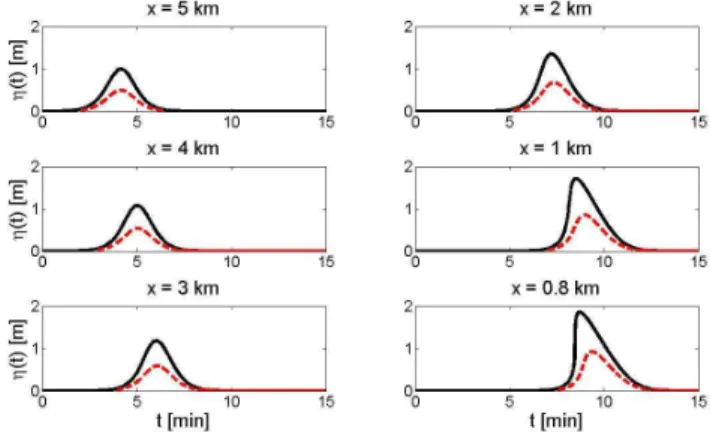
Fig. 1. Time series of nonlinear wave transformation during its propagation to the coast; red dashed line corresponds to the wave withA0=0.5 m, black solid line – toA0=1 m.

The details of the derivation of Eq. (3) can be found in (Di-denkulova, 2009). Equation (3) describes the wave propagat-ing in any onshore or offshore direction. In the case of the wave propagating to the shore, it can be seen from Eq. (3) that the wave increases its amplitude and steepens during the propagation to the coast. The demonstration of this process is shown in Fig. 1 for initial solitary wave with different am-plitudes, located atx0=5 km at the depthh0=40 m

η0(t )=A0cosh−2(t /T0), (4)

whereT0=60 s is the characteristic duration of the wave.

The wave of 1 m height steepens faster than the one of 0.5 m height and breaks at 780 m far from the coast, while the 0.5-m wave breaks 480 m from the coast. The breaking dis-tance (the disdis-tance from the coast, where the wave front be-comes vertical) can also be found from Eq. (3) (Didenkulova, 2009). In the case of the non-reflecting beach Eq. (2) it can be re-written as:

XBr=

x0 h

1+ 8h0√gh0

9A0x0max(η′0)

i3/4, (5)

where the prime means derivative with respect to the argu-ment ofη0in Eq. (3). For a sine wave Eq. (5) has a form

XBr=

x0 h

1+8h0√gh0

9A0ωx0

i3/4. (6)

It follows from Eq. (6) that the wave propagating onshore always breaks.

For the wave propagating seawards (x > x0)the sign of the

second term in argument of the functionη0in Eq. (3) will be

opposite and correspondingly the second term in the denom-inator of the breaking distance Eqs. (5) and (6) should have an opposite sign. As a result, the wave propagating offshore can break only if its amplitude is unrealistically large A0≥

8h0√gh0

9x0max η′0

. (7)

For example, the amplitude of a solitary wave with a 4-min duration propagating offshore from the depth 40 m and dis-tance of 500 m from the coast should be more than 100 m.

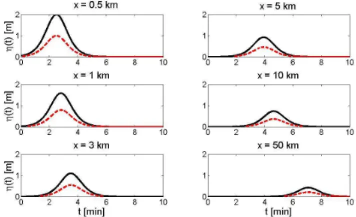
The behavior of 1- and 2-m height waves propagating sea-wards is shown in Fig. 2. It can be seen that, practically, there are no nonlinear effects for the wave propagating offshore.

For different applications it is important to know the wave spectrum and its changes. The spectral characteristics of the nonlinear wave propagating in the basin of constant depth are studied in (Zahibo et al., 2008). Spectral representation of the wave moving onshore in a basin of slowly varying depth can be found from Eq. (3). Let us study a transformation of a sine wave with amplitudeA0and frequencyω[η0=A0sin(ωt )]

along the bottom profile (2). In this case the wave field can be presented as a Fourier series

η(T ,x)₌

∞

X

n₌1

An(x)sin(nωT ), (8)

whereT₌t₋τ (x)and An(x)=

=2_πA0x_x01/3

π

Z

0

sin ωT₊ 9ηωx0 8h0√gh0

x₀

x 4/3

−1 x x0

1/3! ×

×sin(nωT )d (ωT ). (9) Integral in Eq. (9) can be taken and the final expression for spectral amplitudes is

An(x)=

=16h0 √

gh0

9ωnx0

x₀ x

1/3x₀ x

4/3 −1

−1 ×

×Jn

_9A

0ωnx0

8h0√gh0

_x

0

x 4/3

−1

, (10)

whereJn are Bessel functions of then-th order. Using the

breaking distance for a sine wave (6) Eq. (10) can be re-written in the following form:

An(x)=

=2A_n0x_x0

1/3 

 

_x

0 XBr

4/3 −1

x0 x

4/3 −1



 ×

×Jn



 n



 

x0 x

4/3 −1 _x

0 XBr

4/3 −1



  



. (11)

Fig. 2. Time series of nonlinear wave transformation during its propagation seawards; red dashed line corresponds to the wave with

A0=1 m, black solid line – toA0=2 m.

From Eq. (11) we can find proportions between different har-monics and their changes with the time. In particular, at the moment of the first wave breakingx₌XBr, amplitude of the

firstA1and secondA2harmonics are:

A2

A0=

J2(2)

2

_x

0

XBr 1/3

≈0.18

_x

0

XBr 1/3

, A1

A0=

J1(1)

_x

0

XBr 1/3

≈0.44

_x

0

XBr 1/3

. (12)

It follows from Eq. (12) that at the moment of the first wave breaking amplitude of the second harmonicsA2is connected

to the first harmonicsA1in the following way:

A2=

A1J2(2)

2J1(1) ≈

0.4A1. (13)

The results discussed above have been obtained with the use of the nonlinear WKB approximation valid at large distances ∼XBr(Engelbrecht et al., 1988). However, if we apply the

direct perturbation theory to Eq. (3), found with an assump-tion of smoothly varying depth (see Didenkulova, 2009 for details), which is formally valid at distances smaller than XBr, in the second order of the perturbation theory the field

will consist of two harmonics only: η₌A0

x₀ x

1/3

sin(ωT )+

+A0 2

x₀ x

1/3 h _x

0 x

4/3 −1i

x0 XBr

4/3 −1

sin(2ωT ). (14)

Equation (14) can also be obtained from Eq. (12) assuming x_≪XBr.

to this solution. The amplitude of the correction term is pro-portional to the squared initial amplitude and changes with the distance asx−5/3

∼h−5/4_{, which is significantly stronger}

than the Green’s law. So, when the wave approaches the shore the amplitude of the nonlinear correction grows faster than the one of the linear term and the wave tends to break. Of course, this conclusion is valid for both, asymptotic and direct perturbation approaches.

The amplitude of the small nonlinear correctionA2 with

respect to the amplitude of the linear termA1calculated from

Eq. (14) can be expressed as a function of the only parameter

XBr x0

A2

A1=

1 2

h _x

0 x

4/3 −1i

x0 XBr

4/3 −1

, (15)

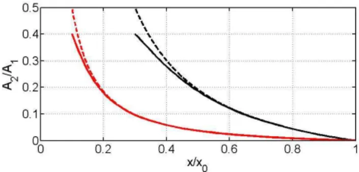
and it is shown in Fig. 3. It can be seen from Eq. (15) that at the breaking distance the amplitude of the second harmonics A2is twice smaller than the amplitude of the first harmonics

A1. Thus, in the vicinity of the wave breaking the

pertur-bation theory overestimates the amplitude of the second har-monics by 20 % compare to the asymptotic approach (13).

Similar analysis can be performed for the wave propagat-ing seawards. In this case amplitudes of harmonics, obtained with the use of asymptotic approach Eqs. (11), and the wave field found from the perturbation theory Eq. (14), should be re-written as

Aoff_n (x)₌2A0 n

x₀ x

1/3 

   

x0 Xoff_Br

4/3 −1

x0 x

4/3 −1



    ×

×Jn



    n



   

x0 x

4/3 −1

x0 Xoff_Br

4/3 −1



    

   

, (16)

ηoff₌A0 x₀

x 1/3

sin(ωT )+

+A0 2

x₀ x

1/3 h _x

0 x

4/3 −1i "

x0 Xoff_Br

4/3 −1

#sin(2ωT ). (17)

It can be seen that in the case of the wave propagating sea-wards the perturbation theory in the vicinity of the wave breaking also overestimates the amplitude of the second har-monics compare to the asymptotic approach.

Fig. 3. Amplitude of the second harmonic A2 with respect to

the amplitude of the first harmonicA1 calculated from Eq. (14)

for XBr

x0 =0.1 (red dashed line) and 0.3 (black dashed line); solid

lines show the corresponding ratio ofA2andA1calculated from

Eq. (11).

3 Non-adiabatic nonlinear effects at the non-reflecting beach

In the general case when the water depth is varied arbitrary, we cannot find neither asymptotic no exact analytical solu-tion of Eqs. (1); this also applies to the non-reflecting beach (2). That is why here in order to describe the nonlinear ef-fects at the non-reflecting beach of an arbitrary slope we use a direct perturbation theory. We should also note that based on the analysis presented in the previous section we expect that the perturbation theory will overestimate the magnitude of the nonlinear correction by up to 20 %.

Let us assume a weakly nonlinear case of Eqs. (1) η₌ηl+ηnl, u=ul+unl, (18)

ηnl≪ηl, unl≪ul, (19)

whereηl andul correspond to the water displacement and

flow velocity in the linear case and ηnl andunl reflect the

influence of the nonlinearity.

When substituting Eq. (18) into Eq. (1) we obtain linear shallow water equations forηlandulto a first approximation:

∂ηl

∂t + ∂

∂x[h(x)ul]=0, ∂ul

∂t +g ∂ηl

∂x =0, (20) and for small nonlinear correctionsηnl andunl we have the

system of linear inhomogeneous equations ∂ηnl

∂t + ∂

∂x[h(x)unl]= − ∂ ∂x[ηlul], ∂unl

∂t +g ∂ηnl

∂x = − 1 2

∂u2_l

∂x. (21)

Equation (21) can be reduced to the inhomogeneous wave equation for the water displacement:

∂2ηnl

∂t2 −

∂ ∂x

gh(x)∂ηnl ∂x

=8(x,t),

8(x,t)₌1 2

∂ ∂x

" h(x)∂u

2 l

∂x #

− ∂

2

For the bottom profile defined by Eq. (2) the general solu-tion of the homogeneous Eq. (22) represents a superposisolu-tion of two travelling waves propagating in opposite directions. Here we consider only one wave propagating shoreward, pre-sented in the complex form (Didenkulova et al., 2009) ηl(x,t )=Al(x)eiωt+A∗l(x)e−

iωt_,

ul(x,t )=Ul(x)eiωt+Ul∗(x)e−

iωt_,

(23) where

Al(x)=

A0

2

_h

0

h(x) 1/4

eiωτ (x)_,

Ul(x)=

A0 2 r _g h(x) _h 0 h(x) 1/4

−1+ √ gh 4hiω dh dx

eiωτ (x)_, (24) Substituting Eq. (24) into Eq. (22) in the right hand side of Eq. (22) we have

8(x,t)₌810(x,t )+811(x,t )e2iωt+8∗11(x,t )e−2iωt,(25)

where 810(x,t )=

d dx h

d_|Ul|2

dx !

,

811(x,t )=

1 2

d dx h

d(U_l2) dx

!

−2iωd(AlUl)

dx . (26) Since the forcing function has three different frequencies then the solution of Eq. (22) should also consists of three terms

ηnl(x,t )=η10(x)+η11(x)e2iωt+η11∗ e−2iωt. (27)

Substituting Eq. (26) into Eq. (22) we obtain two ordinary differential equations for definition of η10(x) and η11(x)

(equation forη∗₁₁(x)is obtained automatically) d

dx

gh(x)dη10 dx

= − d

dx

h(x) d

dx|Ul(x)|

2_,

(28)

d dx

gh(x)dη11 dx

+4ω2η11=

= − " 1 2 d dx h

dU_l2 dx

!

−2iωd(AlUl) dx

#

. (29)

Eq. (27) describes the set-up and set-down effects and can be integrated

η10(x)=C1+

Z _C

2dx

gh(x)−

|Ul(x)|2

g ,C1=

|Ul(x=x0)|2

g ,

C2=0, (30)

coefficientsC1andC2are chosen to satisfy the condition of

no water disturbances before wave arrival and after the wave passage. Equation (28) is the inhomogeneous second-order

Fig. 4.Amplitude of the nonlinear correctionA2with respect to the

amplitude of the linear termA1calculated from Eq. (17) for

X_Broff x0 =

3 (black dashed line) and 5 (red dashed line); solid lines show the corresponding ratio ofA2andA1calculated from Eq. (16).

differential equation with variable coefficients, which can be solved by the method of variation of constants. Let us seek the solution of Eq. (28) in the following form:

η11=H1(x) hx₀

x i1/3

e2iωτ (x)₊H2(x) hx₀

x i1/3

e−2iωτ (x),(31) whereτ is a travel time fromx0andH1(x)andH2(x)are

un-known functions ofx. Substituting Eq. (30) into Eq. (28) we obtain a system for variable amplitudesH1(x)andH2(x):             

dH1(x)

dx e

2iωτ (x)

+dH2(x)

dx e−

2iωτ (x)

=0

dH1(x)

dx e

2iωτ (x)

−dH2(x)

dx e−

2iωτ (x)=

= − A

2 0g

8iω√gh0[ x2₀/3 x8/3−

32√gh0

27iωx3 −

28gh0

81ω2_x10/3_x2/3 0

−

− iωx

4/3 0

3√gh0x7/3+

3ω2_x2 0 gh0x2]e

2iωτ (x)

(32)

from whichH1(x)andH2(x)can be found. In particular, H1(x)=

A2 0g

16iω√gh0

x0

2x2−

32x₀1/3√gh0

63iωx7/3 −

7gh0

54ω2x8/3x₀1/3− iωx5/3₀ 5√gh0x5/3+

9ω2_x7/3 0

4gh0x4/3

−

− A

2 0g

16iω√gh0

1 2x0−

32√gh0

63iωx2−

7gh0

54ω2x3 0−

iω 5√gh0+

9ω2_x 0

4gh0

(33)

and describes a part of second harmonics of the wave propa-gating shoreward. At large distances Eq. (32) behaves like:

H1(x)∼ −

9iωA2₀x0

64h0√gh0 "

x₀4/3 x4/3−1

#

, (34)

which corresponds to 1/4 of the amplitude of the second harmonics found for the wave propagation along the bot-tom of slowly varying depth using the perturbation theory (Eq. 14), and together withH∗

1(x), which is contained in

η∗

11(x)(Eq. 26), they will give a half of it.

In a similar wayH2(x)can be found from Eq. (31) in the

integral form

H2(x)=

Fig. 5.Absolute values ofH₁(x)(black solid line) andH₂(x)(red dashed line) for 1-meter wave propagating shoreward. Blue dash-dotted line corresponds to the amplitude of the second harmonics found for the wave propagation along the bottom of slowly varying depth using the perturbation theory Eq. (14).

×

x

Z

x0

" x0

x3−

32x₀1/3√gh0

27iωx10/3 − (35)

− 28gh0 81ω2_x11/3_x1/3

0

− iωx

5/3 0

3√gh0x8/3+

3ω2x₀7/3 gh0x7/3 #

e4iωτ (x)dx.

It contains components of both incoming and reflected waves, which cannot be separated, and, therefore, describes the nonlinear reflection from the beach which is neglected in the linear approximation.

Both amplitudesH1(x)andH2(x)are displayed in Fig. 5

for 1-m wave propagating shoreward, which is initially lo-cated at the distance 5-km from the coast at the 40 m water depth. For convenience of demonstration Fig. 5 is shown in semi-logarithmic scale.

It can be seen in Fig. 5 thatH2(x)has a quasi-periodic

structure, which confirms the existence of both incident and reflected components inH2(x). Decreasing depth results in

the decrease in the wavelength and spatial period of oscilla-tion when the wave approaches the shore. These changes are close to √h as it could be expected from WKB ap-proach. Since amplitude of waves increases significantly in the coastal zone (in two orders, see Fig. 5) small oscillations are vanished against this background. Amplitude of the sec-ond harmonics found for the wave propagation along the bot-tom of slowly varying depth using the perturbation theory Eq. (14) is larger than sum ofH1(x)andH2(x).

Similar calculations are performed for the 1-m wave prop-agating offshore from the initial distance from the coast of 500 m and the water depth of 40 m. Corresponding ampli-tudesH1(x)andH2(x)are shown in Fig. 6.

Comparison of the second harmonics found from the non-linear WKB approximation (10) and nonnon-linear term (24) is shown in Figs. 7 and 8 for 1-m sine wave propagating shore-ward and offshore respectively. The wave with a period of 4 min is initially located 5 km from the coast (500 m for the wave propagating seawards) at the water depth 40 m. As in

Fig. 6. H1(x)(black solid line) andH2(x)(red dashed line) for

1-meter wave propagating offshore. Blue dash-dotted line corre-sponds to the amplitude of the second harmonics found for the wave propagation along the bottom of slowly varying depth using the per-turbation theory (14).

Fig. 7. Comparison of amplitudes of the second harmonics found from the nonlinear WKB approximation (10) (black solid line) and nonlinear term (26) (red dashed line) for the wave propagating shoreward. Blue dash-dotted line corresponds to the amplitude of the second harmonics found for the wave propagation along the bot-tom of slowly varying depth using the perturbation theory (14).

Fig. 5 it is more convenient to use semi-logarithmic axis in Fig. 7.

Fig. 8. Comparison of amplitudes of the second harmonics found from the nonlinear WKB approximation (10) (black solid line) and nonlinear term (26) (red dashed line) for the wave propagating off-shore. Blue dash-dotted line corresponds to the amplitude of the second harmonics found for the wave propagation along the bottom of slowly varying depth using the perturbation theory (14).

Fig. 9. Wave set-down for the wave propagating shoreward.

nonlinear effects. Variations of the amplitude of the second harmonics in deep water are weak and wave is almost linear. In conclusion let us discuss the effects of wave set-up and set-down (zero harmonics) found from the direct perturba-tion theory (Eq. 29). Its changes for the 1-m wave propa-gating shoreward from 5 km distance from the coast (40 m depth) are shown in Fig. 9. It can be seen that during wave propagation to the coast before the wave breaking, the mean sea level decreases, which leads to the known effect of wave set-down outside the wave breaking zone (Longuet-Higgins and Stewart, 1963; Bowen et al., 1968; Dean and Walton, 2009).

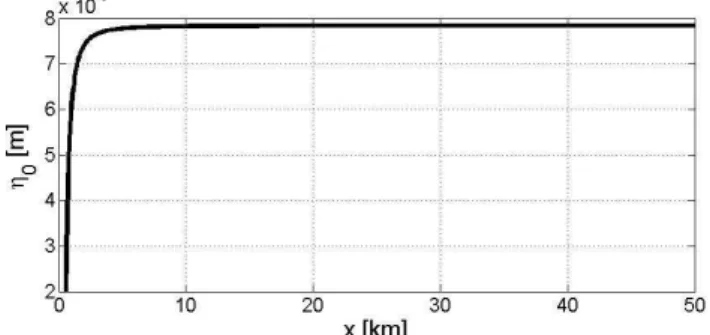
At the same time during wave propagation seaward the mean sea level rises, but those effects are almost negligible. For example, it is shown in Fig. 10 that the seaward propaga-tion of 1-m wave from the initial locapropaga-tion 5 km (depth 40 m) results in less than 1 cm set-up at the distance 50 km from the coast. It also follows from Eq. (29) that the wave set-up for the wave propagation to deep water has an asymptotic and is limited by

η0(x→ ∞)→|

Ul(x=x0)|2

g . (36)

For example, shown in Fig. 10 the maximum set-up is only 8 mm.

Fig. 10.Wave set-up for the wave propagating seaward.

4 Conclusions

Nonlinear evolution of long waves above special bottom pro-file (h∼x4/3)is studied. This profile has a special interest since it allows non-reflecting wave propagation within the linear shallow-water theory; the shape of the wave during its propagation along such a beach is also conserved in time (Didenkulova et al., 2009). At the same time in the nonlinear theory reflection from such a beach exists as it is demon-strated here with the use of the perturbation theory.

It is shown in the framework of the nonlinear WKB ap-proach assuming slow bottom changes and weak nonlinearity that nonlinearity leads to the wave breaking near the coast. In contrary, when the wave propagates seawards it may break only if it is of unrealistically large amplitude. Using direct perturbation theory the generation of zero- and second- har-monics is studied for an arbitrary slope of non-reflecting ge-ometry. It is demonstrated that in the second-order of the per-turbation theory the nonlinearity leads to the wave reflection and change in the sea level. The mean sea level decreases during wave propagation shoreward, which leads to the well-known effect of wave set-down before wave breaking (Dean and Walton, 2009). For the seaward-going wave the mean sea level change is minor and limited by the value, depending on the water flow velocity at the initial location.

Acknowledgements. Partial support from the targeted financing by the Estonian Ministry of Education and Research (grant SF0140007s11), Estonian Science Foundation (grant 8870), RFBR (Grants 11-05-00216, 11-05-92002 and 11-02-00483) and Russian president grant (MK-1440.2012.5) is greatly acknowledged.

Edited by: R. Grimshaw

Reviewed by: two anonymous referees

References

Bjorkavag, M. and Kalisch, H.: Wave breaking in Boussinesq mod-els for undular bores, Phys. Lett. A, 375, 1570–1578, 2011. Bowen, A. J., Inman, D. L., and Simmons, V. P.: Wave set-down

and wave set-up, J. Geophys. Res., 73, 2569–2577, 1968. Caputo, J.-G. and Stepanyants, Y. A.: Bore formation, evolution and

disintegration into solitons in shallow inhomogeneous channels, Nonlin. Processes Geophys., 10, 407–424, doi:10.5194/npg-10-407-2003, 2003.

Carrier, G. F. and Greenspan, H. P.: Water waves of finite amplitude on a sloping beach, J. Fluid Mech., 4, 97–109, 1958.

Dean, R. G. and Dalrymple, R. A.: Coastal processes with engineer-ing applications, Cambridge University Press, 475 pp., 2002. Dean, R. G. and Walton, T. L.: Wave setup, in: Handbook of coastal

and ocean engineering, edited by: Kim, Y. C., World Sci., Singa-pore, 2009.

Didenkulova, I.: Nonlinear long-wave deformation and runup in a basin of varying depth, Nonlin. Processes Geophys., 16, 23–32, doi:10.5194/npg-16-23-2009, 2009.

Didenkulova, I. and Pelinovsky, E.: Non-dispersive traveling waves in strongly inhomogeneous water channels, Phys. Lett. A, 373, 3883–3887, doi:10.1016/j.physleta.2009.08.051, 2009.

Didenkulova, I. and Pelinovsky, E.: Traveling water waves along a quartic bottom profile, Proc. Estonian Ac. Sci., 59, 166–171, doi:10.3176/proc.2010.2.16, 2010.

Didenkulova, I. and Pelinovsky, E.: Runup of tsunami waves waves in U-shaped bays, Pure Appl. Geophys., 168, 1239–1249, doi:10.1007/s00024-010-0232-8, 2011.

Didenkulova, I. and Soomere, T.: Formation of two-section cross-shore profile under joint influence of random short waves and groups of long waves Mar. Geol., 289, 29–33, doi:10.1016/j.margeo.2011.09.011, 2011.

Didenkulova, I., Pelinovsky, E., and Soomere, T: Runup Char-acteristics of Symmetrical Solitary Tsunami Waves of “Un-known” Shapes, Pure Appl. Geophys., 165, 2249–2264, doi:10.1007/s00024-008-0425-6, 2008.

Didenkulova, I., Pelinovsky, E., and Soomere, T.: Long surface wave dynamics along a convex bottom, J. Geophys. Res.-Oceans, 114, C07006, doi:10.1029/2008JC005027, 2009.

Didenkulova, I., Nikolkina, I., Pelinovsky, E., and Zahibo, N.: Tsunami waves generated by submarine landslides of variable volume: analytical solutions for a basin of variable depth, Nat. Hazards Earth Syst. Sci., 10, 2407–2419, doi:10.5194/nhess-10-2407-2010, 2010.

Engelbrecht, J. K., Fridman, V. E., and Pelinovsky, E. N.: Nonlinear Evolution Equations, Pitman Research Notes in Mathematics Series, No. 180, Longman, London, 1988.

Gurtin, M. E.: On the breaking of water waves on a sloping beach of arbitrary shape, Quart. Appl. Math., 33, 187–189, 1975. Kowalik, Z. and Murty, T. S.: Numerical Modelling of Ocean

Dy-namics, Advanced Series on Ocean Engineering, World Scien-tific, Singapore, Vol. 5, 1993.

Liu, P. L.-F., Yeh, H., and Synolakis, C.: Advances in Coastal and Ocean Engineering Advanced Numerical Models for Simulating Tsunami Waves and Runup, World Scientific, 2008.

Longuet-Higgins, M. S. and Stewart, R. W.: A note on wave set-up, J. Mar. Res., 21, 4–10, 1963.

Massel, S. R.: Hydrodynamics of coastal zones. Elsevier, Amster-dam, 1989.

Mei, C. C.: Applied dynamics of ocean surface waves, Singapore, World Scientific, 1989.

Nwogu, O. G.: Numerical prediction of breaking waves and cur-rents with a Boussinesq model, Proc. 25th International Con-ference on Coastal Engineering, ICCE’96, Orlando, 4807–4820, 1996.

Raubenneimer, B. and Guza, R. T.: Observations and predictions of run-up, J. Geophys. Res., 101, 25575–25587, 1996.

Raubenneimer, B., Guza, R. T., and Elgar, S.: Field observations of wave-driven setdown and setup, J. Geophys. Res., 106, 4639– 4638, 2001.

Sato, S. and Kabiling, M. B.: A numerical simulation of beach evolution based on a nonlinear dispersive wave-current model. Proceedings of the 24th International Conference held in Kobe, Japan, Coastal Engineering 1994, New York, 2557–2570, 1995. Sorensen, R. M.: Basic Wave Mechanics, Wiley, New York, 1993. Synolakis, C. E.: The runup of solitary waves, J. Fluid Mech., 185,

523–545, 1987.

Varley, E., Venkataraman, R., and Cumberbatch, E.: The propa-gation of large amplitude tsunamis across a basin of changing depth, I. Off-shore behaviour, J. Fluid Mech., 49, 775–801, 1971. Yeh, H., Liu, P. L.-F., and Synolakis, C.: Long-Wave Runup

Mod-els, World Scientific, 1996.