Stochastic Diffusion of Energetic Ions Due to
Incoherent Lower Hybrid Waves
Lucio M. Tozawa and Luiz F. Ziebell
Instituto de F´ısica, Universidade Federal do Rio Grande do Sul
Caixa Postal 15051, 91501-970, Porto Alegre, RS, Brasil
Received on 9 May, 2003
In the present paper we discuss stochastic diffusion of energetic ions by a set of lower hybrid waves with frequencies close to each other and random phases which change along the time evolution of the system. We obtain efficient long term diffusion in velocity space, which is more representative of the diffusion produced by a continuous wave packet than the diffusion produced by a set of waves with random phases which are constant along the time evolution.
1
Introduction
It is known that the movement of ions in a uniform magnetic field may become stochastic in the presence of a coherent electrostatic wave, if the wave amplitude is sufficiently large [1, 2]. The ensuing diffusion in velocity space may have important consequences, as indicated by relatively recent experiments, which show evidence of interaction between lower hybrid waves and energetic ions in large tokamaks [3, 4]. A parametric analysis has shown that the threshold condition for stochasticity as derived in Ref. [1] is not eas-ily satisfied in present day large tokamaks, although it can be attained in small tokamaks with relatively modest levels of wave power [5]. When the threshold condition is satis-fied a quasilinear formalism can be derived and employed to describe the stochastic diffusion which occurs in veloc-ity space [2]. Using quasilinear analysis, significant wave-particle interaction between energetic ions and lower hybrid (LH) waves has been indeed demonstrated to occur [6, 7].
In a recent paper we have investigated the transition be-tween cases in which one coherent LH wave is present in the system, with amplitude below the stochasticity thresh-old, and cases with the presence of several LH waves of close frequencies, studying the appearance of stochasticity along this transition [8]. We have employed a generaliza-tion of Karney’s approach, assuming that a finite number of waves is present in the system, forming a sufficiently narrow wave packet inkspace [8]. Despite the relative simplicity of the Hamiltonian obtained, the system dynamics has been shown to be complicated, originating interesting behavior which had not until quite recently been widely studied in the literature [9].
The analysis made in Ref. [8] has shown that in the particular case of a set of coherent waves the threshold for stochastic diffusion is reduced in comparison with the threshold in the one wave case, with the ensuing particle diffusion in velocity space occurring in periodic bursts along the time evolution. For a set of waves with random phases, the results appearing in Ref. [8] have shown more
effi-cient long term diffusion in velocity space than in the case of the same number of coherent waves, although the initial diffusion rate for incoherent waves may be smaller than in the case of coherent waves. Reduction of the stochastic-ity threshold regarding the coherent one-wave case has also been obtained in other situations, for instance assuming two waves propagating obliquely to the ambient magnetic field [9], or considering the possibility of a modulation in the wave frequency [10].
In the present paper we resume the use of the theoreti-cal approach employed in Ref. [8], now applied to the case of a finite set of waves with randomly chosen phases that are modified along time evolution. This procedure tends to average out all possibly remaining regularity in the distribu-tion of the wave phases, so that the outcome must be close to that expected for a continuous wave packet.
The structure of the paper is the following. In Sec. 2 we present a summary of the theoretical formalism devel-oped in Ref. [8], which helps to explain fundamental fea-tures of the system and show how to obtain the equations of motion. In Sec. 3 we present some numerical results which illustrate the appearance of stochastic diffusion in the system due to the presence of a set of incoherent lower hy-brid waves, considering both the case of waves with random phases which are fixed along time evolution, and waves with random phases which change along the time evolution of the system. Finally, in Sec. 4 we summarize our findings and comment on the main results of the paper.
2
The description of the system and
the equations of motion
Let us therefore consider the following magnetized system:
B=B0ez
E=X
i
Theωiappearing in this expression are angular frequencies
of the individual waves in a set ofnωwaves, theEi(ωi)are
the amplitudes of these waves, and theφiare their phases.
Assuming the Coulomb gauge,
A=−B0yex,
we can writeE=−∇Φ, with
Φ =−X
i
Ei(ωi)
ki(ωi)
sin (ki(wi)y−ωit−φi)ey. (2)
The Hamiltonian for the system can be written as fol-lows.
h= P 2
2m+qΦ, (3)
where
P2 =p2
x+p
2
y+q
2
B2 0y
2
−2qpxB0y,
and whereqandmare the ion charge and mass respectively, and thepi are the cartesian components of the particle
mo-mentum. We have used pz(t = 0) = 0, which implies
pz(t) = 0.
For the sake of simplicity, we consider thatnωis an odd
number, with waves equally spaced in frequency. We denote the amplitude, the angular frequency and the phases of the central wave asE,ω, andφ, respectively, and assume initial conditions such that the phase of the central wave is zero (φ = 0). Using these definitions, we introduce the dimen-sionless variables
t′= Ωt, Ω =qB0
m , y
′ =k y,
p′
i=
k
mΩpi, (i=x, y) (4) wherek=ki(ωi=ω).
As a consequence of these definitions, the Hamiltonian appears as follows.
h′=1
2
h
(p′
x+y′)
2 +p′2
y
i
−αX
i
rEi
rki
sin (rkiy
′−ν
it′−φi), (5)
where
α= qmE0
k k2 m2Ω2 =
E0
B0
k
Ω =
E0/B0 Ω/k ,
rEi =
Ei(ωi)
E0
,
rki = ki/k, νi = ωi/Ω, and h′ = hm/(mΩ/k)
2 . The amplitudeE0is obtained from the following normalization condition,
E2 0 = 2
*Ã X
i
Eicosϕiey
!
·
X
j
Ejcosϕjey
+
,
whereϕi≡(kiy−ωit−φi), and the symbol< ... >means
the time average over a time interval sufficiently large in order to be an integer multiple of the periods of all waves appearing in thekwave packet. The rate of amplitudesrEi,
therefore satisfies the following constraint
nω
X
i=1
r2
Ei
cos2
ϕi®+2 nω−1
X
i=1
X
j>i
rEirEjhcosϕicosϕji=
1 2. (6) After performing the time average, we obtain
cos2
ϕi®= 0.5, andhcosϕicosϕji= 0.0, and therefore,
from Eq. (6),
nω
X
i=1
r2
Ei = 1. (7)
Also for the sake of simplicity, we consider the case in which thenω waves of the kspace packet have the same
amplitude (rEi=rE, for anyi),
rE= (nω)−
1/2
. (8)
We can also definerωi = ωi/ω, and consider that the
wave spectrum is non-vanishing only betweenω−δωand
ω+δω, and thereforerωi spreads from rωi = 1−∆ to
rωi = 1 + ∆, where∆ = δω/ω. If the wave packet ink
space is narrow, we may assume also for the sake of sim-plicity that for the waves in the packet
ω
k ≃V, (9)
whereV is a constant. As a consequence,
rωi =
ωi
ω =
V ki(ωi)
V ki(ω)
=ki(ωi)
k =rki(ωi),
and therefore
νi =ωi
ω ω
Ω =rkiν, where ν =
ω
Ω.
Dropping the ’primes’, for simplicity, we obtain as the system’s Hamiltonian,
h=1 2
h
(px+y)
2 +p2
y
i
−αX
i
rEi
rki
sin [rki(y−νt−φi)]. (10)
Following steps similar to those employed in Ref. [1], we perform the following canonical transformation
(x, y, px, py)⇒(X, Y, Px, Py)
F2(x, y, Px, Py) = (Px−νt)x+Py(y−νt+Px) (11)
X = ∂F2
∂Px
=x+Py
Y = ∂F2
∂Py
=y−νt+Px
px=
∂F2
py=
∂F2
∂y =Py
K=h+∂F2
∂t =h−ν(x+Py) =h−νX,
resulting
Y =y+px, X =x+py.
The new Hamiltonian is
K(X, Y, Px, Py) =
1 2
£
Y2 +P2
y
¤
−αX
i
rEi
rki
sin [rki(Y −Px)−φi]−νX. (12)
Performing now a second canonical transformation, (X, Y, Px, Py)⇒(I1, ω1, I2, ω2)
F1(X, Y, ω1, ω2) = 1 2Y
2
cotg(ω1) +Xω2.
Px= ∂F
1
∂X =ω2,
Py =∂F
1
∂Y =Ycotg(ω1)→Py= (2I1)
1/2
cos(ω1),
I1=−
∂F1
∂ω1 = 1
2Y 2
cosec2(ω1)→Y = (2I1) 1/2
sin(ω1),
I2=−
∂F1
∂ω2
=−X,
we arrive at the final form of the Hamiltonian, denoted as
H,
H =K+∂F1
∂t =K.
The Hamiltonian is therefore
H =I1+νI2
−αX
i
rEi
rωi
sin{rωi[Rsin(ω1)−ω2]−φi}, (13)
where we have usedrki =rωiand definedR= (2I1)
1/2 . The Hamiltonian equations are easily obtained as fol-lows
˙
ωi=
∂H ∂Ii
, I˙i=−
∂H ∂ωi
,
˙
ω1= 1−sin(ω1) 1
Rα
X
i
rEicos{rωi[Rsin(ω1)−ω2]−φi},
˙
ω2=ν,
˙
I1= cos(ω1)Rα
X
i
rEicos{rωi[Rsin(ω1)−ω2]−φi},
˙
I2=−α
X
i
rEicos{rωi[Rsin(ω1)−ω2]−φi}. (14)
This set of coupled equations is now ready to be object of a numerical analysis, with results presented in Sec. 3.
3
Some numerical results
For the numerical solution of the Hamiltonian equations, we assume a given number of particles (np) and a given
num-ber of waves (nω) and giveαandνas parameters. We also
assume a given value of∆and a distribution of wave ampli-tudesrEi.
As loading procedure for the numerical calculation we initially consider the following case: We give parameters
I0
1,a0, and the initial HamiltonianH, and attribute, for the
npparticles, regularly spaced values ofI1,ω1andω2:
I1=I 0 1+
1
np
a0, I 0 1 +
2
np
a0, ..., I 0 1 +a0,
ω1= 2π 1
np,2π
2
np, ...,2π,
ω2= 2π 1
np
,2π 2 np
, ...,2π,
I2= (H−I1+S)/ν, (15) where
S≡αX
i
rEi
rωi
sin{rωi[Rsin(ω1)−ω2]−φi}.
In other words, the loading procedure assumes initial values forI1,ω1andω2, and evaluateI2, in such a way that all the particles have the same initial Hamiltonian (H), for which we have arbitrarily assumed the valueH =I0
1+νI 0 1. In Ref. [8] we have also considered the same set of par-ticle initial conditions utilized here, and also a different set of initial conditions. The results obtained were qualitatively similar in both cases, indicating that they were not restricted to a special set of conditions.
It is useful to remark here that when assuming the initial value ofI1for each particle, we are simply assuming the ini-tial value of the perpendicular canonical momentum of the particles, since reversing the canonical transformations one obtains
I1= 1 2
k2 m2Ω2
£
p2
y+ (px−qAx)
2¤
,
wherepx andpy are thexandy dimensional components
of the particle momentum, as used in Eq. (3), before the introduction of the dimensionless variables by Eq. (4).
With the choice of parametersI0
1 anda0, the spread of perpendicular momenta of the particles is such that50.0 < R < 57.4, where as we have seenR = √2I1. This range of parameters is similar to that utilized in previous studies of the one-wave case, which we use for comparison when considering the case of several waves [1, 2].
αdependent and have been stablished approximately as the following [1],
Rmin=ν−√α, Rmax= (4αν)2/3(2/π)1/3.
Forν = 30andα= 2.0, the stochasticity therefore will fully occur in the region28.6 < R <33.2. Forα= 4.0, in the region 28.0 < R < 43.5, and forα = 6.0, in the region27.5 < R < 69.0. Therefore, for our choice of pa-rameters, in the one-wave case small amount of stochastic-ity may be expected for α = 2.0, for instance, since the range 50.0 < R < 57.4 is far from the stochastic range, and appreciable amount of stochasticity forα= 4.0, since the range50.0< R <57.4is close to the stochastic range. On the other hand, for larger wave amplitude, as in the case of α = 6.0, for instance, one can expect fully stablished stochasticity in the chosen range, which will be completely immersed in the stochastic region. These expectations will be now subjected to numerical confirmation, and compared to the case of fixed wave amplitude and different number of incoherent waves.
We start by considering the one-wave case, same situa-tion considered in Refs. [1] and [2].
In order to illustrate the effect of the increase of the wave intensity, we present in Fig. 1 the quantityRversusω2(mod. 2π), for the case of 50 particles and one wave, withα=2.0, 3.0, 4.0, and 5.0, assumingI0
1 = 1.25×10 3
,a0= 400, and
ν = 30.0. The sequence of panels illustrates the gradual modification of particle trajectories caused by the increase in the wave intensity. It is seen the gradual appearance of the overlap of particle orbits which has been shown to cor-respond to stochastic diffusion in velocity space [1, 2].
48 50 52 54 56 58 60 62
0 1 2 3 4 5 6 7
R
ω2
(a)
48 50 52 54 56 58 60 62
0 1 2 3 4 5 6 7
R
ω2
(b)
48 50 52 54 56 58 60 62
0 1 2 3 4 5 6 7
R
ω2
(c)
48 50 52 54 56 58 60 62
0 1 2 3 4 5 6 7
R
ω2
(d)
Figure 1. Ras a function ofω2(mod. 2π), for 50 particles, one wave (nω = 1),ν = 30, and (a)α= 2.0, (b)α=3.0, (c)
α=4.0, and (d)α=5.0.
We now consider the presence of more than one wave, with different frequencies and random phases which are fixed in time, with the phase of the central wave assumed to be zero (φ = 0). The random phases are obtained from a random number generator which starts from a numerical seed. All the results which follow, unless explicitly stated otherwise, are generated with the use of the same seed for the random number generator.
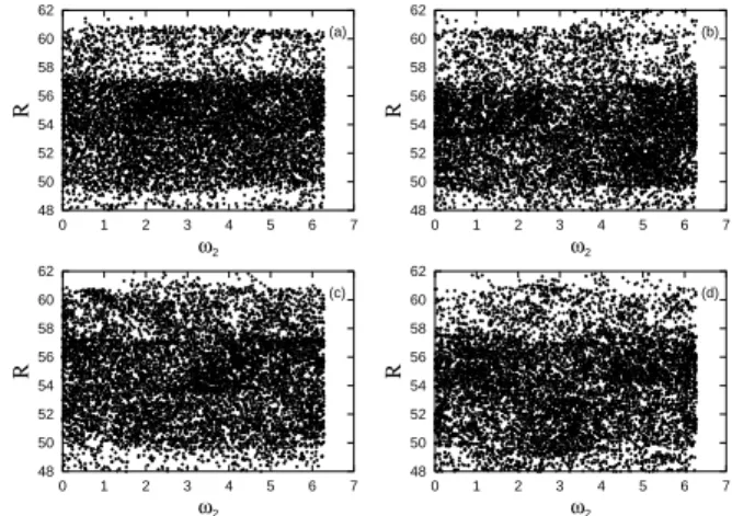
In Fig. 2 it is seen the case ofRversusω2 (mod. 2π), considering 50 particles andα= 2.0, for several values of
the number of waves (1, 3, 5, and 7), using∆ = 1.0×10⁻² and the other parameters as in Fig. 1. Figure 2 clearly shows that the presence of the waves with random phases cause the complete spreading of the particle orbits which are present in the case of only one-wave, for the same value ofα.
48 50 52 54 56 58 60 62
0 1 2 3 4 5 6 7
R
ω2
(a)
48 50 52 54 56 58 60 62
0 1 2 3 4 5 6 7
R
ω2
(b)
48 50 52 54 56 58 60 62
0 1 2 3 4 5 6 7
R
ω2
(c)
48 50 52 54 56 58 60 62
0 1 2 3 4 5 6 7
R
ω2
(d)
Figure 2. Ras a function of ω2 (mod. 2π), for 50 parti-cles and waves with fixed random phases,α= 2.0,ν = 30, ∆ = 1.0×10⁻²
, and number of waves (a) 1, (b) 3, (c) 5, and (d) 7.
48 50 52 54 56 58 60 62
0 1 2 3 4 5 6 7
R
ω2
(a)
48 50 52 54 56 58 60 62
0 1 2 3 4 5 6 7
R
ω2
(b)
48 50 52 54 56 58 60 62
0 1 2 3 4 5 6 7
R
ω2
(c)
48 50 52 54 56 58 60 62
0 1 2 3 4 5 6 7
R
ω2
(d)
Figure 3. Ras a function of ω2 (mod. 2π), for 50 parti-cles and waves with fixed random phases,∆ = 1.0×10⁻²
,
nω= 5, and (a)α= 0.25, (b)α= 0.5, (c)α= 1.0, and (d)α=
2.0.
In Fig. 3 we show R as a function of ω2 (mod. 2π), for the case in which five waves are present in the sys-tem, considering smaller values of the wave amplitude (α= 0.25,0.5,1.0,and2.0), and ∆ = 1.0×10⁻²
The presence of stochastic behavior can also be investi-gated by following the time behavior of the following quan-tities,
(δIj)t=
(
1
np−1 np
X
i=1
[Ij(t)−Ij(0)]
2
)1/2
, (16)
wherej = 1,2. In a plot of(δIj)tversust, the inclination
of(δIj)trelative to thetaxis is a measure of the diffusion
coefficient in velocity space [11].
In Fig. 4 we show (δI1)t as a function of normalized time, forI0
1 = 1.25×10 3
,a0 = 400,ν = 30.0, andα = 2.0, for nω= 1, 5, and 9, for the case of waves with
ran-dom phases which are fixed in time. For this figure, we have considerednp = 1000, which results in much better
statis-tics than obtained withnp = 50. The Poincar´e plots
pre-sented in Figs. 1 to 3, on the other hand, were obtained with
np = 50because with a larger number of particles it
be-comes very difficult to see any structure in the plots, due to the proximity of the dots which represent sucessive passages of particles by the Poincar´e section. Panel (a) shows the evo-lution up tot≃120, while panel (b) shows the evolution up tot ≃1200. According to Fig. 4, the long term evolution of the quantity(δI1)tappearing in Fig. 4b shows continued diffusion, without the conspicuous “steps” appearing in the case of coherent waves [8].
0 20 40 60 80 100 120
0 20 40 60 80 100 120
(
δ
I1
)t
t (a)
0 50 100 150 200 250 300
0 200 400 600 800 1000 1200
(
δ
I1
)t
t (b)
Figure 4. (δI1)t as a function of normalized time, for the
case of waves with fixed random phases, forI0
1 = 1.25× 10³
,a0= 400,ν = 30.0, andα=2.0, fornω= 1 (full line),
5 (broken line), and 9 (dotted line). (a) Short-term evolution; (b) Long-term evolution.
Figure 4 has been obtained for a given set of random phases. If a different seed would be attributed to the random number generator, a different set of random phases would be obtained, which would result in different time evolution for the quantity depicted in the figure. We have obtained results for different sets of initial random phases, some of which have been displayed in Ref. [8]. What we have served from these different cases is that, although the ob-vious differences between the different curves obtained, the inclination relative to thetaxis is approximately the same in all corresponding cases, indicating similar average diffu-sive behavior. The interesting parameters for the emulation of the interaction of a narrow wave packet with energetic particles seem to be the wave energy and the width of the spectrum, and not the particular phases of the waves com-posing the finite set of waves chosen to arbitrarily represent the spectrum. These results could be in principle improved by an ensemble average, considering a large number of sets of random phases, which would require very intensive use
of numerical calculation. It is expected that the average be-havior obtained using different sets of random phases would tend to become more and more similar for increasing num-ber of waves, so that in the limit of infinite wave numnum-ber the difusion caused by the waves would be independent of the particular set of random phases utilized in the calcula-tion. Instead of proceeding with this costly approach, we may consider the case of a finite set of waves, with randomly chosen phases that are modified along time evolution, which tend to average out all possibly remaining regularity in the phase distribution, so that the outcome must be close to that expected for a continuous wave packet.
We now consider the presence of more than one wave, with different frequencies and random phases which are modified along the time evolution, with the initial phase of the central wave assumed to be zero (φ = 0). The phases are modified after a real time interval which aver-agesδt= 2π/δω, so that for longer time intervals all phase correlations are averaged out. In nondimensional time, for ∆ = 1.0 ×10⁻²
andν = 30.0, the modification of the phases occurs after an average intervalδt≃20. The effect of the finite set of waves becomes truly random and more adequate to the emulation of a wave packet of finite width.
48 50 52 54 56 58 60 62
0 1 2 3 4 5 6 7
R
ω2
(a)
48 50 52 54 56 58 60 62
0 1 2 3 4 5 6 7
R
ω2
(b)
48 50 52 54 56 58 60 62
0 1 2 3 4 5 6 7
R
ω2
(c)
48 50 52 54 56 58 60 62
0 1 2 3 4 5 6 7
R
ω2
(d)
Figure 5. R as a function of ω2 (mod. 2π), for 50 par-ticles and waves with random phases which change along time evolution,α= 2.0,ν= 30,∆ = 1.0×10⁻²
, and num-ber of waves (a) 1, (b) 3, (c) 5, and (d) 7.
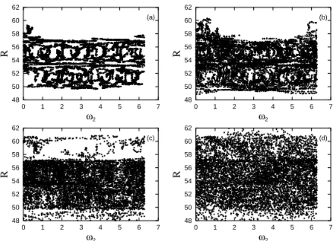
For this situation, in Fig. 5 it is seen the Poincar´e plot of
Rversusω2(mod. 2π), again considering 50 particles and
α= 2.0, for several values of the number of waves (1, 3, 5, and 7), using∆ = 1.0×10⁻²
and the other parameters as in Fig. 1. Except for the random phases which change along time, these are exactly the same conditions used to gener-ate Fig. 2. Fig. 5 clearly shows that the randomly changing phases cause the complete spreading of the particle orbits which appeared in the fixed phase one-wave case, result-ing in a plot which appears qualitatively independent of the number of the waves, at least for the region in phase space which is depicted in Fig. 5.
wave amplitude (α= 0.25,0.5,1.0,and2.0, the same val-ues considered for Fig. 3), and∆ = 1.0×10⁻²
. The loading procedure and other parameters are also the same. We ob-serve that the amount of stochastic diffusion, for the same number of iterations, is gradually smaller for smaller wave energy, but even in the case ofα= 0.25 the degree of stochas-ticity is larger than that obtained in the one-wave case and
α= 2.0, seen in the first panel of Fig. 1 and in the first panel of Fig. 2. Comparing the first panel of Fig. 6 with the first panel of Fig. 3, it is seen that the randomness of the phases is responsible for significant diffusive behavior which was pratically absent in the corresponding case ofα= 0.25for five waves with fixed phases.
48 50 52 54 56 58 60 62
0 1 2 3 4 5 6 7
R
ω2
(a)
48 50 52 54 56 58 60 62
0 1 2 3 4 5 6 7
R
ω2
(b)
48 50 52 54 56 58 60 62
0 1 2 3 4 5 6 7
R
ω2
(c)
48 50 52 54 56 58 60 62
0 1 2 3 4 5 6 7
R
ω2
(d)
Figure 6. R as a function of ω2 (mod. 2π), for 50 par-ticles and waves with random phases which change along time evolution,∆ = 1.0×10⁻²
,nω= 5, and (a)α= 0.25,
(b)α= 0.5, (c)α= 1.0, and (d)α= 2.0.
0 20 40 60 80 100 120
0 20 40 60 80 100 120
(
δ
I1
)t
t (a)
0 50 100 150 200 250 300
0 200 400 600 800 1000 1200
(
δ
I1
)t
t (b)
Figure 7. (δI1)tas a function of normalized time, for the
case of waves with random phases that change along time evolution, forI0
1 = 1.25×10 3
,a0 = 400,ν = 30.0, and
α=2.0, fornω= 1 (full line), 5 (broken line), and 9 (dotted
line). (a) Short-term evolution; (b) Long-term evolution. Proceeding along the proposed line, in Fig. 7 we show (δI1)tas a function of normalized time, forI
0
1 = 1.25×10 3
,
a0 = 400, ν = 30.0, and α =2.0, fornω= 1, 5, and 9,
for the case of waves with random phases that change along time evolution. As for Fig. 4, the number of particles has been assumed to be 1000. The long-term evolution depicted at panel (b) at the right-hand side shows that the stochas-ticity introduced by the randomly changing waves results in continued diffusive behavior in velocity space, even for the one wave case.
In Fig. 8 we show(δI1)t as a function of normalized time, for the one-wave case (nω = 1),I10 = 1.25×10
3 ,
a0 = 400,ν = 30.0, andα =2.0, 3.0, 4.0, and 5.0, con-sidering that the phase of the wave changes randomly along the time evolution. Panel (a) of Fig. 8 shows the evolution up to normalizedt≃120, and panel (b) shows the extended evolution, up tot ≃1200. Fig. 8 clearly shows that long-term diffusive behavior, measured by the inclination of the curve relative to thetaxis, is nearly proportional to the wave amplitude, while it should be nearly absent in the region of the phase space depicted in the figure, forα ≃ 2.0, if the phase of the wave were kept constant along time evolution, according to the analysis presented at the beginning of the present section.
0 20 40 60 80 100 120 140 160 180
0 20 40 60 80 100 120
(
δ
I1
)t
t (a)
0 50 100 150 200 250 300 350 400 450 500
0 200 400 600 800 1000 1200
(
δ
I1
)t
t (b)
Figure 8. (δI1)t as a function of normalized time, for
nω = 1,I10 = 1.25×10 3
,a0 = 400,ν = 30.0, andα= 2.0 (full line), 3.0 (broken line), 4.0 (dashed line), and 5.0 (dotted line). The phase of the wave is randomly modified along time evolution. (a) Short-term evolution; (b) Long-term evolution.
4
Final remarks
We have generalized the discussion on stochastic diffusion of energetic ions by lower hybrid waves by considering a case where a set of waves with similar frequencies and ran-dom phases which change ranran-domly along time evolution is present in the system. As in Ref. [8], the task has been accomplished by generalization of the approach utilized in Refs. [1, 2] under the restriction that the spectra is suffi-ciently narrow such that the phase velocity of the waves present in the system can be considered to be a constant. The present discussion generalizes previous results obtained assuming a set of waveswith fixed phases, since the random modification of the phases along time evolution tends for long time evolution to be equivalent to an ensemble average over fixed phases, which would be much more costly from a numerical point of view.
The results obtained indicate significant long term diffu-sion which is nearly independent from the number of waves present in the system. The random modification of the phases along time evolution averages possible regularities originated from a given set of phases, and produces stochas-tic diffusion which must be close to that expected from a continuous wave packet of finite fequency width.
Acknowledgments
References
[1] C. F. F. Karney, Phys. Fluids 21, 1584 (1978). [2] C. F. F. Karney, Phys. Fluids 22, 2188 (1979).
[3] M. C. R. de Andrade, M. Brusati, and the JET team, Plasma Phys. Contr. Fusion 36, 1171 (1994).
[4] D. Testa et al., Plasma Phys. Contr. Fusion 41, 507 (1999).
[5] L. F. Ziebell and L. M. Tozawa, Braz. J. Phys. 28, 222 (1998). [6] L. M. Tozawa and L. F. Ziebell, Braz. J. Phys. 28, 211 (1998).
[7] L. F. Ziebell, Plasma Phys. Contr. Fusion 42, 359 (2000).
[8] L. M. Tozawa and L. F. Ziebell, Phys. Rev. E 66, 056409, 13p. (2002).
[9] S. Benkadda, A. Sen, and D. R. Shklyar, Chaos 6, 451 (1996).
[10] S. Riyopoulos, Phys. Fluids 28, 1097 (1985).