SRef-ID: 1607-7946/npg/2005-12-117 European Geosciences Union
© 2005 Author(s). This work is licensed under a Creative Commons License.
Nonlinear Processes
in Geophysics
Nonlinear multidimensional scaling and visualization of earthquake
clusters over space, time and feature space
W. Dzwinel1, D. A. Yuen2, K. Boryczko1, Y. Ben-Zion3, S. Yoshioka4, and T. Ito5
1AGH Institute of Computer Science, al. Mickiewicza 30, 30-059, Krak´ow, Poland 2Minnesota Supercomputing Institute, Univ. of Minnesota, Minneapolis, MN 55455, USA 3Department of Earth Sciences, University of Southern California, Los Angeles, CA 90089, USA 4Department of Earth and Planetary Sciences, Kyushu University, Fukuoka, 812-8581, Japan
5Graduate School of Environmental Studies, Nagoya, University, Furo-cho, Nagoya, Aichi, 464-8602, Japan
Received: 4 October 2004 – Revised: 1 December 2004 – Accepted: 2 December 2004 – Published: 28 January 2005
Abstract. We present a novel technique based on a multi-resolutional clustering and nonlinear multi-dimensional scal-ing of earthquake patterns to investigate observed and syn-thetic seismic catalogs. The observed data represent seis-mic activities around the Japanese islands during 1997–2003. The synthetic data were generated by numerical simulations for various cases of a heterogeneous fault governed by 3-D elastic dislocation and power-law creep. At the highest res-olution, we analyze the local cluster structures in the data space of seismic events for the two types of catalogs by using an agglomerative clustering algorithm. We demon-strate that small magnitude events produce local spatio-temporal patches delineating neighboring large events. Seis-mic events, quantized in space and time, generate the multi-dimensional feature space characterized by the earthquake parameters. Using a non-hierarchical clustering algorithm and nonlinear multi-dimensional scaling, we explore the multitudinous earthquakes by real-time 3-D visualization and inspection of the multivariate clusters. At the spatial resolu-tions characteristic of the earthquake parameters, all of the ongoing seismicity both before and after the largest events accumulates to a global structure consisting of a few separate clusters in the feature space. We show that by combining the results of clustering in both low and high resolution spaces, we can recognize precursory events more precisely and un-ravel vital information that cannot be discerned at a single resolution.
1 Introduction
Understanding of earthquake dynamics and development of forecasting algorithms require a sound knowledge and skill in both measurement and analysis spanning various geo-physical data, such as seismic, electromagnetic, gravita-tional (Song and Simons, 2003), geodetic, geochemical, etc.
Correspondence to:D. A. Yuen
The Gutenberg-Richter power-law distribution of earthquake sizes (Gutenberg and Richter, 1944) implies that the largest events are surrounded (in space and time) by a large number of small events (e.g. Wesnousky, 1994; Ben-Zion and Rice, 1995; Wiemer and Wyss, 2002). The multi-dimensional and multi-resolutional structure of this global cluster depends strongly on geological and geophysical conditions (Miller et al., 1999; Ben-Zion and Lyakhovsky, 2002), past seis-mic activities (Rundle et al., 2000, 2002), closely associ-ated events (e.g. volcano eruptions) and time sequence of the earthquakes forming isolated events, patches, swarms etc.
Investigations on earthquake predictions are based on the assumption that all of the regional factors can be filtered out and general information about the earthquake precursory patterns can be extracted (Geller et al., 1997). This extrac-tion process is usually performed by using classical statisti-cal or pattern recognition methodology. Feature extraction involves a pre-selection process of various statistical proper-ties of data and generation of a set of seismicity parameters (Keilis-Borok and Kossobokov, 1990; Eneva and Ben-Zion, 1997a, b), which correspond to linearly independent coordi-nates in the feature space. The seismicity parameters in the form of time series can be analyzed by using various pat-tern recognition techniques ranging from fuzzy sets theory and expert systems (e.g. Wang and Gengfeng, 1996), multi-dimensional wavelets (Enescu et al., 2002; Erlebacher and Yuen, 2001, 2003) to neural networks (Joswig 1990; Dowla 1995; Tiira, 1999; Rundle et al., 2002; Anghel et al., 2004).
Prediction of earthquakes is a very difficult and challeng-ing task (Geller et al., 1997); we cannot operate only at one level of resolution. The coarse graining of the original data can destroy the local dependences between the events and the isolated earthquakes by, e.g. neglecting their spatio-temporal localization. In coarse-grain analysis, the subtle correlations between the earthquakes and preceding patches of events can vanish in the background of uncorrelated and noisy data.
F F F F F FF
FEEEEEEEEAAAAAAAATTTTTTTTUUUUUUUURRRRRRRREEEEEEEE SSSSSSSSPPPPPPPPAAAAAAAACCCCCCCCEEEEEEEE YYYYYYYY
Y Y Y
Y={Yj: Yj =[Yj1, Yj2 ..., YjN]} D
DAATTAA SSPPAACCEE XX
X ={Xi: Xi = [Xi1, Xi2, ..., Xin ]}
F Feeaattuurreeggeenneerraattiioonn
X→→→→YYYY Yjl →→→→ Flj(Xi)
M u l t i d i m en si on a l sc a l i n g
Y YY Y→→→→ZZZZ (Yj→→→→Zj)
S S S S S SS
SPPPPPPPPAAAAAAAACCCCCCCCEEEEEEEE OOOOOOOOFFFFFFFF EEEEEEEEXXXXXXXXTTTTTTTTRRRRRRRRAAAAAAAACCCCCCCCTTTTTTTTEEEEEEEEDDDDDDDD FFFFFFFFEEEEEEEEAAAAAAAATTTTTTTTUUUUUUUURRRRRRRREEEEEEEESSSSSSSS ZZZZZZZZ
Z Z Z
Z = {Zj; Zj = [Zj1, Zj2,, Zj3]}
F FF F F F F
Feeeeeeeeaaaaaaaattttttttuuuuuuuurrrrrrrreeeeeeee ssssssssppppppppaaaaaaaacccccccceeeeeeee
v vv v
v vv viiiiiiiissssssssuuuuuuuuaaaaaaaalllllllliiiiiiiizzzzzzzzaaaaaaaattttttttiiiiiiiioooooooonnnnnnnn
C
Clluusstteerriinnggiinn
d
daattaassppaaccee
DATA MINING AN D KNOWLEDGE EXTRACTION
D
DAATTAA AACCQQIISSIITTIIOONN
Xik - measure ment k for
event i Data base transactions
C C C C C C C Clllllllluuuuuuuusssssssstttttttteeeeeeeerrrrrrrriiiiiiiinnnnnnnngggggggg iiiiiiiinnnnnnnn
ffff
ffffeeeeeeeeaaaaaaaattttttttuuuuuuuurrrrrrrreeeeeeee ssssssssppppppppaaaaaaaacccccccceeeeeeee
D
Daattaassppaaccee
v
viissuuaalliizzaattiioonn
Fig. 1. The principal steps of the knowledge extraction process. The data spaceX is represented by n-dimensional vectorsXi of measurementsXk. It is transformed to a new abstract spaceY of vectorsYj. The coordinatesYl of these vectors represent seismic parameters, which are nonlinear functions of measurementsXk. The new featuresYlformN-dimensional feature space. The dimensional scaling procedure is used for visualizing the multi-dimensional events in 3-D space for a visual inspection of theN -dimensional feature space.
seismicity catalogs. In Dzwinel et al. (2003), we proposed a new approach employing clustering for multivariate anal-ysis of seismic data. The method can extract local spatio-temporal clusters of low magnitude events and recognize cor-relations between the clusters and the large earthquakes. We showed that these clusters could reflect clearly the short-term trends in seismic activities followed by isolated large events. However, local clustering of seismic events is not sufficient to extract an overall picture concerning the precursory pat-terns.
Our analysis procedure does not use a standard software package. Our goal is to construct an interactive system for data mining (Mitra and Acharya, 2003), which allows one to match the most appropriate clustering schemes for the struc-ture of actual seismic data. As shown in Figs. 1 and 2, our data-mining techniques include not only various clustering algorithms but also feature extraction and visualization tech-niques. This present approach is more general than the work of (Dzwinel et al., 2003).
In this paper we propose a novel muti-resolutional ap-proach, which combines local clustering techniques in the data space with a non-hierarchical clustering in the feature space. The raw data are represented byn-dimensional vec-torsXiof measurementsXk. The data space can be searched
for patterns and be visualized by using local or remote pat-tern recognition and advanced visualization capabilities. The data spaceXis transformed to a new abstract spaceYof vec-torsYj. The coordinatesYl of these vectors represent
non-linear functions of measurementsXk,which are averaged in
space and time in given space-time windows. This transfor-mation allows for coarse graining of data (data quantization),
D
DAATTAASSPPAACCEE
fi = [xi, zi, ti, mi]
VISUALIZATION
IN POSITION-TIME-MAGNITUDE SPACE
AGGLOMERATIVE CLUSTERING
Produces clusters of similar events fi
C
COOAARRSSEEGGRRAAIINNIINNGG
7
7--DD FFEEAATTUURREE SSPPAACCEE
Fj = [NSj, NLj, CDj, SRj, AZj, TIj, MRj]
where the coordinates are the seismicity parameters defined in the paper
NON-HIERARCHICAL CLUSTERING MULTIDIMENSIONAL SCALING NON-LINEAR TRANSFORMATION
3D ←←←← 7-D VISUALIZATION
IN 3-D FEATURE SPACE
H
HIIGGHHRREESSOOLLUUTTIIOONN
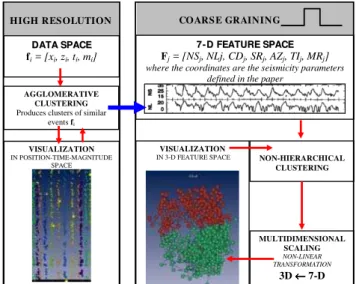
Fig. 2.Schematic diagram of multi-resolutional analysis of seismic events. At the highest level of resolution, a single seismic eventi
is represented as a multi-dimensional data vectorfi. These vec-tors contain information about local properties of seismic patterns. A general knowledge about the data has to be extracted from the lower resolution feature spaceby using coarse graining proce-dureL[8]. The MDS transformationMS[]→ωmaps the 7-D feature spaceinto its image in a 3-D spaceω.
amplification of their characteristic features, and suppres-sion of both the noise and other random components. The new featuresYl form anN-dimensional feature space. We
use multi-dimensional scaling procedures for visualizing the multi-dimensional events in 3-D space. The Sammon’s non-linear transformation (Jain and Dubes, 1988) (multidimen-sional scaling), transformsYinto a 3-DZspace of extracted features, assuming that this dimensionality reduction mini-mizes the distortions between the N-dimensional structure ofYj vectors and its 3-D image inZspace. This
transfor-mation allows for a visual inspection of theN-dimensional feature space. The visual analysis helps greatly in detecting subtle cluster structures, not recognized by classical cluster-ing techniques, selectcluster-ing the best pattern detection procedure used for data clustering, classifying the anonymous data and formulating new hypotheses.
We used our methodology for analyzing the observed (Ito and Yoshioka, 2002; Toda et al., 2002) and synthetic (Ben-Zion, 1996) earthquake data. The observed data represent seismic activity of the Japanese islands in the 1997–2003 time interval. The synthetic catalogs correspond to various cases of a large heterogeneous fault zone in an elastic half-space.
ap-proach can indeed improve greatly the accuracy of following the evolution of earthquake dynamics. Finally, we discuss the conclusions and future prospects.
2 Methodologies
2.1 Multi-resolutional analysis of multidimensional seis-mic data
In Fig. 2, we show that the seismic data can be analyzed in diverse resolutions, associated with two different types of spaces:
1. The first is the data space 8 with data vectors fi
(i=1,...,N) – which correspond to the data describing a single seismic event.
2. The second one, more abstract, is the feature space
of time eventsFj (j=1,...,M) andM≪N – an
ab-stract space resulting from a non-linear transformation
L[8]→ representing the feature generation proce-dure.
At the highest level of resolution, a single seismic eventican be represented as a multi-dimensional data vectorfi=[mi, zi,xi,ti] wheremi is the magnitude andxi,zi,ti – its
epi-central coordinates, depth and the time of occurrence, re-spectively. As shown in (Dzwinel et al., 2003), we can an-alyze these data locally by looking for clusters with similar (or dissimilar) events using the agglomerative clustering pro-cedures (Andenberg, 1973; Gowda and Krishna, 1978; Jain and Dubes, 1988; Theodoris and Koutroumbas, 1998). The search for similar data is limited to successive time stripestk
with the same width1τ. We are seeking neighbors of event
ionly intk and the previoustk−1time intervals. The pointj
belongs to the nearest neighbors of eventiif a given set of conditions is fulfilled (see Dzwinel et al., 2003). This allows us to identify correlated patches of events that reflect short-term trends in seismic activity initiated by rapid changes gen-erated by strong events. By combining similarity and dis-similarity measures (Theodoris and Koutroumbas, 1998) be-tween the data vectors, we can extract also the patches of small magnitude events corresponding to the isolated large earthquakes. This type of data analysis extracts information on the local properties of seismic patterns (Dzwinel et al., 2003). However, this also generates a large number of extra-neous clusters, which produce unreliable information over a long timescale.
With the above procedure, we cannot extract general knowledge about the data, which requires the detection of long-range spatial and temporal correlations. This knowl-edge has to be extracted from a global data structure in a low resolution space. We achieve this by using a coarse graining procedureL[8]. This averages out the noise and detailed modes of the data vector components.
The coordinates in the low resolution feature space are de-fined by means of seismicity parameters. Originally they are
computed as timeτ and spaceX averages in a given time [t0, tEND] and space intervals ([X0, XEND]=[x0, xEND] ∪
[z0,zEND] – epicentral coordinates and depth, respectively)
within a sliding time window with a length1T and time step
dt, i.e.
αi = tEND
Z
t0
Z
X∈[X0,XEND]
α (τ, X)·H (t0+i·dt, τ )dτ dX (1)
H (t, τ )=
1 for -1T2 < τ−t < 1T2
0 otherwise , (2)
where αrepresents one of the following seismicity param-eters: N S, N L, CD, SR, AZ, T I, MR. The value of dt
was assumed to be equal to the average time difference be-tween two recorded consecutive events while 1T is equal to about 1/10 of the average time distance between two suc-cessive large events (for synthetic data m>6, for real data
m>5). Larger values ofdt and1T give smoother time se-ries due to better statistics. However, by increasingdt and
1T poorer prediction characteristics can be expected. The seismicity parameters are defined as follows (Eneva and Ben-Zion, 1997a, b):
Degree of spatial non-randomness at short (N S) and at long distances (N L) – represents the differences between distributions of event distances and distances between ran-domly distributed points. NS and NL represent the portions of events involved in anomalies in short distances and long distances, respectively (0–5 km and 60–65 km for the syn-thetic catalogs, Eneva and Ben-Zion, 1997).
1. Spatial correlation dimension (CD) - calculated on the basis of correlation integrals based on interevent dis-tances.
2. Degree of spatial repetitiveness (SR) – contains the spatio-magnitude. components and represents the ten-dency of events with similar magnitudes to have nearly the same locations of hypocenters.
3. Average depth (AZ).
4. Inverse of seismicity rate (T I) – time interval in which a given (constant) number of events occurs.
5. Ratio of the numbers of events falling into two different magnitude rangesMR=N (m≥M0)/N (m<M0).
We have introduced an additional parameterM, which is not used in the data processing and simply displays the maxi-mum magnitude of events in the moving time window.
We focus our data analysis on the time series of seven seis-micity parameters that create the abstract 7-dimensional fea-ture space of time eventsFt = (N St,N Lt,CDt,SRt,AZt, T It, MRt) where t are discretized values of time. These
all the 7 parameters in the same moment of time. Because the number of clusters is generally unknown, and most of the clustering methods are not able to extract the clusters of com-plicated shapes and densities accurately (Ertoz et al., 2003), we propose to visualize the clustering structure in the feature space. We use multi-dimensional scaling transformationMS
[]→ω, which maps the 7-D feature spaceinto its image in a 3-D spaceω(Jain and Dubes 1988; Siedlecki et al., 1988; Theodoris and Koutroumbas, 1998; Dzwinel, 1994; Dzwinel and Blasiak, 1999). From high-resolution 3-D visualization, one can discern clearly how strong the clusters are and how they are positioned with respect to each other. This allows us to fine tune the clustering parameters or select a different clustering algorithm that matches better the clustered struc-tures.
2.2 Clustering schemes
Clustering analysis is a mathematical concept whose main useful role is to extract the most similar (or dissimilar) sep-arated sets of objects according to a given similarity (or dis-similarity) measure (Andenberg, 1973). This concept has been used for many years in pattern recognition. Nowadays clustering and other feature extraction algorithms are recog-nized as important tools for revealing coherent features in the earth sciences (Rundle et al., 1997, 2000; Freed and Lin, 2001), bioinformatics (Jones and Pevzner, 2004) and in data mining (Xiaowei et al., 1999; Grossman et al., 2001; Hand et al., 2001; Hastie et al., 2001; Mitra and Acharya, 2003). Depending on the data structures and goals of classification, different clustering schemes must be applied (Gowda and Kr-ishna, 1978; Karypis and Kumar, 1999).
In our new approach we use two different classes of clus-tering algorithms for different resolution levels. In data space we use agglomerative schemes, such as modified mu-tual nearest neighbor algorithm (mnn) (Gowda and Krishna, 1978; Karypis et al., 1999; Boryczko et al., 2003). This type of clustering extracts better the localized clusters in the high-resolution data space.
In the feature space we are searching for global clusters of time events comprising similar events from the whole time interval. The non-hierarchical clustering algorithms are used mainly for extracting compact clusters by using global knowledge about the data structure. We use improved k-means based schemes (Theodoris and Koutroumbas, 1998), such as a suite of moving schemes (Ismail and Kamel, 1989), which uses the k-means procedure plus four strategies of its tuning by moving the data vectors between k-clusters to ob-tain a more precise location of the minimum of the goal func-tion:
J (Z)=X j
X
i∈Cj
xi−zj
2
, (3)
whereZ=[z1, ...,zk],zjis the position of the center of mass
of the clusterj, whilexiare the feature vectors closest tozj.
To find a global minimum of functionJ (), we repeat many times the clustering procedures for different initial
condi-tions. Each new initial configuration is constructed in a spe-cial way from the previous results by using the methods from (Ismail and Kamel, 1989; Zhang and Boyle, 1991). The clus-ter structure with the lowestJ (w, z)minimum is selected. 2.3 Multidimensional scaling (MDS)
The feature extraction methods, called also mapping tech-niques or multi-dimensional scaling (MDS), represent lin-ear or non-linlin-ear transformations of N-dimensional data into
n-dimensional sets, where n≪N (Jain and Dubes, 1988; Siedlecki et al., 1988; Theodoris and Koutroumbas 1998; Dzwinel, 1994; Dzwinel and Blasiak, 1999). These meth-ods allow for visualization of the multidimensional data in 3-D and for participating interactively the process of cluster extraction.
The MDS algorithm, which is based on the “stress func-tion” criterion, is one of the most powerful mapping tech-niques. The goal is to maintain all the distances between pointsRi∈ω⊂ℜN in the Euclidean 3-D (or 2-D) space with a minimum error. The “stress function” criterion is as fol-lows:
E ω, ω′=X j <iD
−wm ij ·
Dij−rij′ d
=min, (4)
where:
rij′ = ri−rj· ri−rj, i, j =1, ..., M.
Di,j– is a squared distances between pointsRi,Rj∈ω⊂ℜN
andri,rj∈ω′⊂E3 – coordinates of the respective points in
3-D Euclidean space andw,d– parameters.
The result of mapping depends on the quality of the mini-mum obtained for the criterion function (Eq. 4). The dimen-sionality of the “stress function” domain is very high and is equal toN·M(thousands, in typical problems). An increase of the number of input data (more than 103), the dimension-ality of source space and data complexity may cause the re-sulting 2-D (3-D) patterns to be completely illegible. This is often the case with application of standard numerical algo-rithms for finding minimum of this multimodal, non-linear and complex criterion. To make the non-linear mapping use-ful for visualization of greater (M>103 and N >102) data samples, a new minimization technique extracting global minimum of the criterion function is required.
We propose to use the molecular dynamics algorithm (Dzwinel and Blasiak, 1999) as a solver, which can be used for finding the global minimum of the criterion function (Eq. 4). Let us assume that:
1. an initial configuration ofMmutually interacting “par-ticles” is generated inE3,
2. every “particle” corresponds to the respective N -dimensional point fromℜN,
3. the “particles” interact with each other with 8i,j
(a)
z x
time
(b)
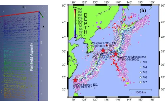
Fig. 3. (a)The synthetic raw data (horizontal distance –X, depth –z) visualized in time by using the Amira visualization package (http: //www.amiravis.com) for A data set (Ben-Zion, 1996). Large events (m>6) are shown as distinctly larger dots on the background of low magnitude events (m<4). There are visualized patches of low magnitude events preceding larger events (Dzwinel et al., 2003). The patches represent clusters marked in colors.(b)Seismic activities around the Japanese Archipelago within 5 years time period. We use the hypocentral data provided by the Japan Meteorological Agency (JMA). The magnitude of the earthquakes (JMA magnitude) and their depths are represented by differences of the radius of the circle and colors, respectively. The red stars symbolize large events such as: Chi-Chi Taiwan earthquake (21 September 1999 M7.6 latitude 23.8 longitude 121.1) Swarm at Miyakejima (July 2000– August 2000 latitude 34.0 longitude 139.0) Western Tottori earthquake (6 October 2000 M7.3 latitude 35.3 longitude 133.4).
8i,j = k
2mD
−wm ij ·
Dij−rij′ d
(5) andkis a stiffness factor. Thus the interaction between each pair of particles is described by various long range poten-tials, dependent on the separation distance between particles
rijand the distanceDij between respective multidmensional points inℜN. To assure the energy dissipation from the sys-tem, an additional friction force is introduced. Using the “leap-frog” numerical scheme (Haile, 1992) the following formula for velocities and positions of “particles” can be de-rived from the momentum equation:
vni+1/2=(1−ϕ) (1+ϕ)·v
n−1/2
i +
α1t (1+ϕ)·
(M
X
j=1
rijn−Dij
d−1
rnij
)
,
rni+1=rni +vni+1/2·1t, (6)
α= k
m, ϕ = λ
2m·1t,
wherevni,rni – the velocity and position of particlei, respec-tively,n– time-step number,m=1 – particle mass.
As it is in molecular dynamics (Haile, 1992), the system of “particles” described by the discrete Eqs. (6) evolves in time according to the Newton equations of motion until the global (or close to the global) minimum of Eq. (5) is reached. Only two free parameters,λandk, have to be fit to obtain the proper stable state, where the final positions of frozen “particles” reflect the result of N-D to 3-D mapping.
3 Description of the data
We analyze the observed and synthetic earthquake catalogs for different time intervals. The synthetic catalogs (Fig. 3a) were obtained by numerical simulations of seismicity on a heterogeneous fault governed by 3-D elastic dislocation the-ory, power-law creep and boundary conditions corresponding to the central San Andreas Fault (Ben-Zion, 1996).
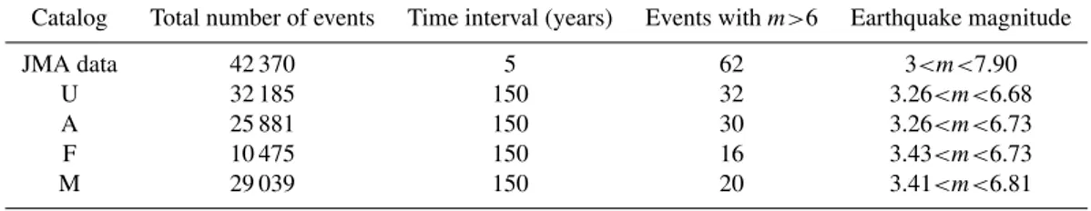
Table 1.Data specification.
Catalog Total number of events Time interval (years) Events withm>6 Earthquake magnitude
JMA data 42 370 5 62 3<m<7.90
U 32 185 150 32 3.26<m<6.68
A 25 881 150 30 3.26<m<6.73
F 10 475 150 16 3.43<m<6.73
M 29 039 150 20 3.41<m<6.81
Original data
Randomized data
M M M M T I T IT I T I
T I T I T I T I
M M M M
TIME
TIME
Fig. 4.The seismicity parametersT IandMfor the “original” and “randomized” synthetic data sets (set A). There is not any correla-tions betweenMandT Ifor the randomize data. This is a contrast to the original data set.
width1T and shiftdt (see Eqs. 1–2). We employ1T=10 days anddt=2 days for the Japanese data and1T=10 months anddt=2 months for the synthetic data. Each parameter in the clustering was normalized with respect to the standard deviation.
The observed data (see Fig. 3b) represents seismic activ-ities of the Japanese islands collected by the Japan Mete-orological Agency (JMA). The JMA catalogue consists of 915 829 events detected in Japan Islands between 1923 and 31 January 2003. The original catalogue includes also events with magnitudes less then 1.0. The lowest magnitudes were determined by using a detection level, estimated from the Gutenberg-Richter frequency-size distribution. For the pur-poses of this paper we have assumed that the cutoff magni-tude of earthquake is equal to 3 (m>3). We do not use any cutoff depth of hypocenter events. The seismic events shown in Fig. 3b, were recorded during the 5 years time interval from 1 October 1997 to 31 January 2003. The data set pro-cessed consists of 42370 seismic events with magnitudesm, position in space (latitudeX, longitudeY, depthz) and oc-currence timet. Statistical completeness of the earthquakes above the detection level assures that no significant events in both space and time are missing.
4 Results of clustering
As shown in Fig. 3a and in (Dzwinel et al., 2003), the syn-thetic seismic events with magnitudesm<4 produce
stripe-like clusters in the data space. They precede large earth-quakes (m>6) and are separated in time by the regions of quiescence. Similar pattern can be observed in the feature space.
In Fig. 4 we display the time series for two, out of seven, seismicity parameters: the maximum magnitude of events in the moving time windowM and the inverse seismicity rate
T I, which define the time distribution of events. The seis-micity parameters were computed both for the raw data set A from the synthetic data catalog (“original data”) and for the same data set but randomized in time (“randomized data”). These two sets of data were searched for clusters in the 7-D feature space . For simplicity, only two clusters were considered. They are represented in Fig. 4 by red and white stripes.
As shown in Fig. 4, theM andT I time series from the “original data” are highly correlated. The periodic occur-rence of large events withm>6 is preceded by the increase of the inverse of seismicity rate T I (the region of quies-cence), which drops at the large event time. Similar corre-lations can be seen for other seismicity parameters not dis-played in Fig. 4. The time intervals corresponding to these rapid changes of seismicity parameters produce one cluster (white), while the rest of them belong to the second cluster (red). Moreover, the periodic stripes representing time in-tervals from the second cluster correspond to the clusters of events in the data space displayed in Fig. 3a. This shows that the averaged properties of a variety of clusters from the data space (see Fig. 3a) are similar, producing a single superclus-ter in the feature space.
It is obvious that clusters can be also found for the “ran-domized data”, however, they are completely meaningless – i.e. computed in-cluster average correlations are statistically irrelevant. This can be inspected visually in Fig. 4. The relations between seismicity parameters – including the cor-relation between the inverse of seismicity rateT I and the averaged magnitudeM – do not exist for the “randomized data”. It is also impossible to extract any distinct proper-ties separating the two clusters (e.g. by using the Karhunen-Loeve transformation, see e.g. Theodoris and Koutroumbas, 1998).
clustering schemes, respectively. These patterns contain in-formation concerning the correlations between characteris-tic features of seismic measurements and their temporal se-quencing. This can be confirmed further by additional anal-ysis of both the synthetic and observed seismic data.
In Fig. 5 we display the seismicity parameters in time com-puted for the complete synthetic data catalog A. The time eventsFt=(N St,N Lt,CDt,SRt,AZt,T It,MRt)produce
3 clusters in the feature space: the first cluster symbolized by green, the second by white and the third by red strips. From the top plot of Fig. 5 displaying the largest eventsM in the sliding time window, we may conclude that the white and red clusters comprise time eventsFt, which correspond to
post mainshock effects. The white cluster represents the net aftershock events while the red one includes the earthquake effects averaged in the sliding time window. Conversely, the green cluster contains the time eventsFtpreceding the
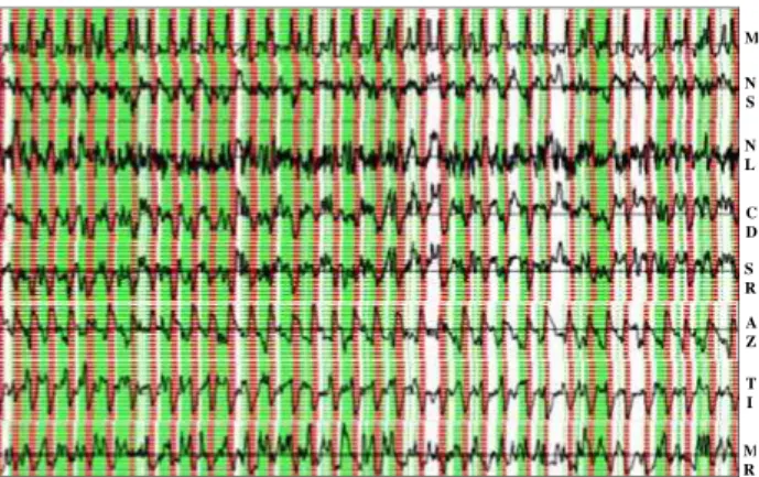
earth-quakes. The selectivity in time of the seismicity parameters depends on the width 1T and shift dt of the sliding time window. Due to space and time averaging, it is impossi-ble to correlate precisely the appearance of a given earth-quake with the rest of the seismicity parameters when two earthquakes are too close to each other. Therefore, the se-quence of green-red-white cluster events can be broken for the time domains with many large earthquakes (see Fig. 5). As shown in Fig. 5, the occurrence of the largest events cor-relates well with the minima ofN S,CD,SR,T I and max-ima ofAZ,MRparameters. This means that the occurrence of large earthquakes is preceded by increasing spatial diffu-sion of events and increasing inverse of seismicity rate. More specifically, the results reveal:
1. an increasing spatial randomness of seismic events, 2. a high spatial correlation dimension (this drops rapidly
at the onset of large events),
3. a decreasing tendency of events with similar magnitudes to have nearly the same locations of hypocenters, 4. a decreasing average depth of seismic activity,
5. an increase of inverse seismicity rate before large events (it drops rapidly at the onset of large event).
For the synthetic data the clusters in the feature space reflect well both the precursory and post mainshock effects. How-ever, the interpretation of clusters for the real data is more complicated and ambiguous.
Results of clustering of the observed Japanese seismic cat-alogs both in data and in feature spaces are shown in Fig. 6. At the highest resolution level a single seismic eventican be represented as a multi-dimensional data vectorfi=[mi,zi, Xi,Yi,ti] where: mi is the magnitude,Xi – the latitude,Yi
– the longitude,zi andti – the depth and the time of
occur-rence, respectively. The seismic events are visualized with the Amira visualization package (http://www.amiravis.com) in Figs. 5a and 5b as an irregular cloud consisted of colored dots with (z,x,t) coordinates.
M
N S
N L
C D
S R
A Z
T I
M R
Fig. 5.The seismicity parametersM,N S,N L,CD,SR,AZ,T I,
MRin time (see Eqs. 1–2) for synthetic data catalog A.
From the Gutenberg-Richter relationship, the number of events of different range of magnitudes differs con-siderably. Therefore, we divide the entire set of data into three subsets comprising the small S (mi<ma),
mediumM(ma≤mi<max) and the large magnitude events L(mi>max). The last ones represent the earthquakes and
are displayed in Figs. 5a and 5b as larger spheres. The deep-est earthquakesz>150 km are not displayed in the Fig. 5. The various shades represent the magnitudes of earthquakes from m=6 (green) to m=7 (red). In Figs. 5a and 5b we present the clustering results in the data space8of the data vectorsfi∈S(mi<ma) (Fig. 5a) andfi∈M(ma≤mi<max)
(Fig. 5b). We have chosen arbitrarily thatma=4 and max=6. We look for clusters of similar events as shown in (Dzwinel et al., 2003). The dots (data vectors), belonging to the same clusters, have the same color.
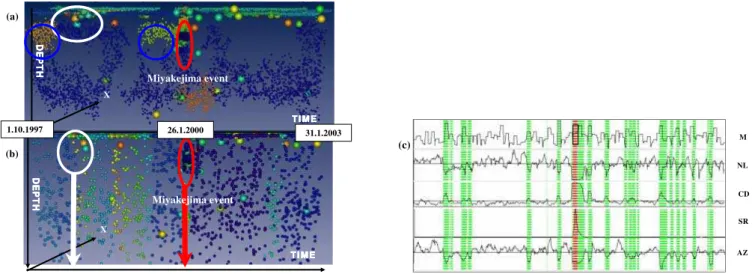
As shown in the upper part of Fig. 6a, clusters made of small size events are located mainly close to the surface (0– 30 km deep). They form long disparate stripes along the time axis. The stripes break-out close to the largest cluster of earthquakes – the Miyakejima event (Toda et al., 2002; Ito and Yoshioka, 2002) – located in the middle of time interval and encircled in red in Fig. 6a. The large swarm of earth-quakes (26 June 2000) occurs in the region of Miyakejima, Honshu, in central Japan (Toda et al., 2002; Ito and Yoshioka, 2002). The eruptions of Miyakejima and five large earth-quakes with magnitudes 6.0 and above occurred together with a large number of 100 000 smaller earthquakes.
Miyakejima event
Miyakejima event
T I M E T I M E T I M E T I M E
D
E
P
T
H
D
E
P
T
H
D
E
P
T
H
D
E
P
T
H
X
T I M E T I M E T I M E T I M E
D
E
P
T
H
D
E
P
T
H
D
E
P
T
H
D
E
P
T
H
X
1.10.1997 26.1.2000 31.1.2003
(a)
(b)
M
NL
CD
SR
AZ
(c)
Fig. 6.Natural seismic data (Ito and Yoshioka, 2002) analyzed by using multi-resolutional clustering in both the data and the feature spaces
(a)–(c). In panels a and b one can see the results of clustering in the data space for small magnitude (3<m<4) and medium magnitude (4<m<6) events, respectively, represented by the small shaded dots. The different colors of the dots mean different clusters. Large events are visualized by the larger spheres. The shades show difference in magnitudesm(red – the largest, green - the smallest). The clusters in panels a-b encircled in red and white shows the places of the largest seismic activity, while those in blue probably represent the clusters of precursory events. The red, white and green stripes in panel c representing 4 (out of 7) seismic parameters and maximum magnitudeM
show the time events belonging to three different clusters. The earthquakes are visualized by using the 3-D Amira visualization package (http://www.amiravis.com).
medium events (4<m<6) (Fig. 6b) have completely different structures. They look like stripes, which lie parallel to X–z plane. The borders between clusters roughly correspond to the borders of successive showers of the earthquakes.
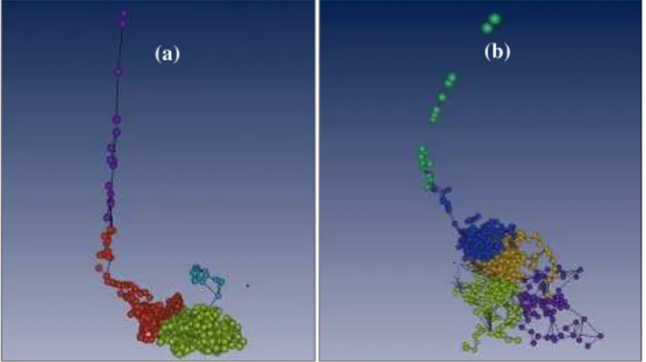
By clustering the time events in the feature space and simultaneous inspection of the results by using multi-dimensional scaling, we have found 4 distinct clusters. The cluster structure in 7-D feature space is shown in Fig. 7a, which represents the result of its mapping into 3-D. The blue cluster forming a long thin rod in Fig. 7a, corresponds to the famous Miyakejima earthquake swarm (Toda et al., 2002) encircled in red on Figs. 6a and 6b. The red and flat clus-ter from Fig. 7a, represent both the largest earthquakes and corresponding time events. The yellow and blue clusters con-tain the rest of the time events. The small blue cluster from Fig. 6a represents the events at the end of the time interval, which are averaged within a shrinking time window. In sum-mary, clustering of averaged time events in the feature space does not detect any anomalies reflecting the precursory pat-terns.
In Fig. 6c we display the time series of selected seismic-ity parameters and in Fig. 7b the 3-D image of the feature space. Both pictures represent the data pre-selected initially by clustering the raw seismic events in the data space. Only small and medium events belonging to the largest clusters (displayed in Figs. 6a and 6b) were used for computing the seismicity parameters. Neglecting the events that do not pro-duce clusters in the data space, we repro-duce the number of un-correlated events both in space and in time enhancing ex-tremes in the time series of seismicity parameters. As shown in Figs. 7a and 7b, in comparison to the original data, the
feature space becomes more diverse producing several well separated clusters. In Fig. 6c, we show that by clustering data in the feature space, we can extract not only Miyake-jima event (red cluster in the center) but also the cluster of events which are characterized by similar behavior of the seismicity parameters as the Miyakejima swarm (green clus-ter). The remaining data produce the white cluster. As shown in Fig. 6c, the green cluster comprises time events corresponding mainly to the largest and shallow earthquakes, which are characterized by increasing randomness of event locations, low spatial correlation dimension which increases rapidly in the moment of large shock, high spatial repetitive-ness and high seismicity rate. The last properties are oppo-site to those observed for the synthetic catalog A. The dif-ferences are caused by the association of the two data sets with very different seismic regimes. Comparing the proper-ties of red, green and white clusters we can conclude that the large swarm in the observed data is preceded and followed by events of a similar nature but considerably smaller mag-nitude. We note that the number of aftershocks is greater than the number of precursory effects belonging to the same green cluster.
The above results cannot be used yet for earthquake pre-diction. It is impossible to forecast earthquakes from just a single case. However, continuing analysis of this type may help to find “dangerous” seismic patterns and predict salient aspects of their evolution.
(a) (b)
Fig. 7. The results of non-linear multi-dimensional scaling of 7-D clusters from the feature spaces defined by the seismicity parame-ters computed for all the seismic events from the data space to 3-D metric space(a)and the same data pre-selected initially by clus-tering(b). The figures are rendered using the Amira visualization package (http://www.amiravis.com).
precursory events produce distinct clusters in both Fig. 4 and Fig. 5, we can construct a simple visual classifier (Jain and Dubes 1988; Theodoris and Koutroumbas 1998) for recog-nizing the precursory patterns.
The entire time interval in the feature space has been di-vided into two parts. The events from the first 2/3 of the in-terval – approximately 700 events – represent the “teaching set”, the rest – about 300 events – make up the “test set”. From the “teaching set” we extract two uneven groups of events. The first one consisting of 10 successive time events preceding each of the earthquake (m>6) is shown in green in Fig. 8. The rest of the events represent the second (pink) cluster from Fig. 8. The clusters are visualized by using multi-dimensional scaling in 3-D. Then, the distances (see Eqs. 3–4) between events belonging to the same clusters was multiplied by the factorλ<1, while the distances between events from different clusters remain the same. The value of
λis gradually decreasing to the moment when the two clus-ters separates from each other. For the situations shown in Fig. 8λis set to 0.8. The events from the “test set” (the blue points) are added to this “teaching” structure, with the de-termined coordinates in 3-Dωspace. They are “attracted” or “repelled” from the “teaching” clusters according to their distances to the events from the “teaching set”. Eventually, we obtain the configurations shown in Fig. 8. The precur-sory events from the test set marked in blue (10 events pre-ceding the earthquake) were recognized at 100% level for synthetic data sets A, U, F. The blue points fall into the area occupied by the green cluster representing precursory events from the “teaching set”. They can be classified by using sim-ple k-NN (k nearest neighbors) classifier. We see that many other points are also situated in the area of a green cluster. However, the choice of precursory events for training was completely arbitrary. By using a more careful analysis of seismicity patterns, such as in (Eneva and Ben-Zion, 1997a), and a better selection of “teaching” patterns, we can improve the classification.
(a) (b)
Fig. 8.Results from visual classification of the synthetic data (from catalogs A and F, respectively) in the feature space transformed into 3-D space by using multi-dimensional scaling (MDS). The time events are divided onto two groups of data (Fi;i<T) (violet and green) and (Fi;i>T) (red and blue) representing: teaching and test sets, respectively. The classifier is constructed using teaching set of time events, which consists of two groups of events: preceding the earthquakes (green) and the others (violet). The preceding time events were taken arbitrarily as the 10 nearest events to the corre-sponding earthquake. In the result of training we obtain two clus-ters: green and violet. The same two groups of data are marked in the test set (preceding the earthquakes – blue, and the others – red). We see that all the blue points were attracted to the green cluster – taught initially as the cluster consisting of “precursory” events -so all of them can be recognized as “precur-sory” (e.g. using k-NN classifier). This is visualized using the authors’ own package and the borders of clusters are drawn manually.
5 Conclusions
The problem of earthquake prediction, based on data extrac-tion of precursory phenomena, is a highly challenging task. Various computational methods and tools are used for de-tection of precursors by extracting general information from noisy data. In our opinion, such a generalization is impossi-ble when the data analysis is carried out at a single level of resolution. Improved possibilities exist when using a set of data-mining tools interactively, allowing for on-line cluster-ing, feature extraction and visualization of the data on vari-ous levels of resolution.
We show that by using a common framework of clustering, we are able to perform multi-resolutional analysis of seis-mic data starting from the raw data events described only by their magnitude-spatio-temporal data space. Then we look for global cluster structure in the feature space, which is de-fined by using the seismicity parameters. This global view can also be divided over different levels of resolution in the feature space defined, e.g. by wavelet analysis (Holschnei-der, 1995; Strang and Nguyen, 1996) of the time series of the seismicity parameters (Torrence and Compo, 1998) and fur-ther classification of wavelet amplitudes by using clustering schemes.
grained feature space by eliminating the noisy patterns and uncorrelated events. We have developed a new software that is based on pre-clustering. This allows for the detection of precursory events with a higher accuracy (e.g. pick-up the Miyakejima event) and their generalization at the low resolu-tion level. It also allows us to construct visual classifiers for anonymous data. We believe that a more careful extraction of the precursory events will be needed for constructing more accurate classifiers.
The raw seismic data contain both local and global knowl-edge of the correlations between the seismic events. Thus, the two-level approach presented here can still be incom-plete, since the general knowledge about the seismic back-ground can be buried in the subtle patterns of data events. Any coarse graining of the data can destroy some, if not a majority, of these patterns. Therefore, extracting global knowledge about seismic patterns corresponding to precur-sory events involves global clustering of data without any averaging. This is a very daunting task both methodolog-ically and computationally. In particular, great difficulties are associated with the irregular structure of seismic data, which comprise many noisy events, different accuracy of measurements, outliers, bridges, clusters of different density and the large number of data vectors (greater than 104) which have to be processed. This problem can be attacked by us-ing modern non-hierarchical clusterus-ing schemes, such as the DBSCAN (Sander et al., 1998), CURE (Guha and Rastogi, 1998), CHAMELEON (Karypis, 1999) or the shared nearest neighbor clustering algorithm (SNNCA) (Ertoz, 2003).
This new methodology can be also used for the analysis of the data from other geological phenomena, e.g, we can apply this clustering method to volcanic eruptions (Amelung et al., 2000; Hong et al., 2004), astrophysical events such as dissipation phenomena, occurring in a dispersed stellar popu-lation (Briceno et al., 2001) also in data mining and bioinfor-matics (Kuramochi and Karypis, 2001; Jones and Pevzner, 2004).
Glossary
– featuresdenotedfi orFj (i, j– feature indices) – a set
of variables which carry discriminating and characteriz-ing information about the objects under consideration. The features can represent raw measurements (data)fi
or can be generated in a non-linear way from the data
Fj (features).
– data vector (fkwherek– data vector index) and
fea-ture vector (Fk wherel– feature vector index) – a
col-lection of features ordered in some meaningful way into multi-dimensional column vectorsfk andFl that
resents the signature of the object to be identified rep-resented by raw datafi or generated featuresFj. The
dimensionalities of data and feature vectors can be dif-ferent.
– data space – the multidimensional space in which the data vectorsfk exist.
– feature space– the multidimensional space in which the Fk vectors are defined. Data and feature vectors
represent multidimensional points in respective spaces. – class – the category to which a given object belongs.
The classes can create patterns in a properly defined multidimensional space.
– cluster – isolated set of multidimensional points (ob-jects) in data and feature spaces.
– clustering – the computational procedure extracting clusters in multidimensional spaces.
– agglomerative clustering algorithm – the algorithm of a clustering procedure in which the clusters are built-up in a hierarchical way. At the start of clustering, the multidimensional points represent singular clusters. The procedure repeats the process of gluing-up the clos-est clusters to the moment when a proper number of clusters is achieved.
– non-hierarchical clustering algorithm – the cluster-ing algorithm in which the clusters are searched for by using global optimization algorithms (unlike in ag-glomerative clustering where local search is exploited). The most representative algorithms of this type are con-structed on the base of k-means procedure.
– k-means clustering (Theodoris and Koutroumbas, 1998) – non-hierarchical clustering algorithm in which the randomly generated centers of clusters are then im-proved iteratively. This simple idea is exploited in vari-ous variants of this algorithm.
– multi-resolutional clustering analysis – due to clus-tering a hierarchy of clusters can be obtained. The anal-ysis of the results of clustering in various resolution lev-els allows for extraction of knowledge hidden in both local (small clusters) and global (large clusters) similar-ity of multidimensional points (objects).
– data mining(Mitra and Acharya, 2003) – algorithms, tools, methods and systems used in extraction of knowl-edge hidden in a large amount of data.
Acknowledgements. We acknowledge the Japan Meteorological
Agency (JMA), which allowed us to use their hypocentral data set We thank George Karypis, Y. J. B. D. Kaneko Zack, A. Garbow, B. J. Kadlec, E. Bolling and G. Erlebacher for useful discussions and K. Tiampo for valuable comments and remarks. WD and KB acknowledge support from the Polish Committee for Scientific Research (KBN) Grant No. 3T11C05926. DAY acknowledges support from both the Geophysics and the ITR programs. YBZ acknowledges support from a Mercator fellowship of the German Research Society (DFG).
Edited by: G. Z¨oller
References
Amelung, F., Jonsson, S., Zebker, H., and Segall, P.: Widespread uplift and ‘trapdoor” faulting on Galapagos volcanoes observed with radar interferometry, Nature, 407, 993–996, 2000. Andenberg, M. R.: Clusters Analysis for Applications, New York,
Academic Press, 1973.
Anghel, M., Ben-Zion Y., and Martinez, R. R. : Dynamical system analysis and forecasting of deformation produced by an earth-quake fault, Pure Appl. Geophys., 161, 2023–2051, 2004. Ben-Zion, Y. and Rice, J. R.: Slip patterns and earthquake
popula-tions along different classes of faults in elastic solids, J. Geophys. Res., 100, 12, 12 959–12 983, 1995.
Ben-Zion, Y.: Stress, slip and earthquakes in models of com-plex single-fault systems incorporating brittle and creep defor-mations, J. Geophys. Res., 101, 5677–5706, 1996.
Ben-Zion, Y. and Lyakhovsky, V.: Accelerated seismic release and related aspects of seismicity patterns on earthquake faults , Pure Appl. Geophys., 159, 2385–2412, 2002.
Boryczko, K., Dzwinel, W., and Yuen, D. A.: Clustering Revealed in High-Resolution Simulations and Visualization of Multi-Resolution Features in Fluid-Particle Models, Concurr. Comp-Pract., 15, 101–116, 2003.
Briceno, C., Vivas, A. K., Calvet, N., Hartmann, L., Pacheco, R., Herrera, D., Romero, L., Berlind, P., Sanchez, G., Snyder, J. A., and Andrews, P.: The CIDA-QUEST Large-Scale Survey of Orion OB1: Evidence for Rapid Disk Dissipation in a Dispersed Stellar Population, Science, 291, 93–96, 2001.
Dowla, F. U.: Neural networks in seismic discrimination, in Mon-itoring a CTBT, edited by Husebye E. S. and Dainty, A. S., NATO-ASI series E 303, Kluwer Publishing, 777–789, 1995. Dzwinel, W.: How to Make Sammon’s Mapping Useful for
Multi-dimensional Data Structures Analysis?, Pattern Recogn., 27/7, 949–959, 1994.
Dzwinel W. and Blasiak, J.: Method of particles in visual clustering of multi-dimensional and large data sets, Future Gener. Comp. S., 15, 365–379, 1999.
Dzwinel, W., Yuen, D. A., Kaneko, Y., Boryczko, K., and Ben-Zion, Y.: Multi-Resolution Clustering Analysis and 3-D Visualization of Multitudinous Synthetic Earthquakes, Vis. Geosc., 8, 12–25, 2003.
Eneva, M. and Ben-Zion, Y.: Techniques and parameters to an-alyze seismicity patterns associated with large earthquakes, J. Geophys. Res., 102, 177 85–17 795, 1997a.
Eneva, M. and Ben-Zion, Y.: Application of pattern recognition techniques to earthquake catalogs generated by models of seg-mented fault systems in three-dimensional elastic solids, J. Geo-phys. Res., 102, 24 513–24 528, 1997b.
Enescu, B., Ito, K., and Struzik, Z.: (Multi)fractality of Earthquakes by use of Wavelet Analysis. Proceedings of American Geophys-ical Union Fall Meeting, 6–10 December 2002, San Francisco, California, 2002.
Erlebacher, G. and Yuen, D. A.: A Wavelet Toolkit for Visualization and Analysis of Large Data Sets In Earthquake Research, Pure Appl. Geophys., 161, 2215–2229, 2004.
Erlebacher, G., Yuen, D. A., and Dubuffet, F. W.: Current trends and demands in visualization in the geosciences, http://link.springer-ny.com/link/service/journals/10069/technic/ erlebach/index.htm, Electr. Geosc., 4, 2001.
Ertoz, L., Steinbach, M., and Kumar, V.: Finding Clusters of Differ-ent Size, Shapes and Densities in Noisy, High-Dimensional Data, Army High Performance Center, technical report, April 2003.
Freed A. M. and Lin, J.: Delayed triggering of the 1999 Hec-tor Mine earthquake by viscoelastic stress transfer, Nature, 411, 180–183, 2001.
Geller, R. J., Jackson, D. D., Kagan, Y. Y., and Mulargia, Y. F.: Earthquakes Cannot Be Predicted, Science Online, 275, 5306, 1616, 1997.
Gowda, C. K. and Krishna, G.: Agglomerative clustering using the concept of nearest neighborhood, Pattern Recogn., 10, 105–112, 1978.
Grossman, R. L., Karnath, Ch., Kegelmeyer, P., Kumar, V., and Namburu, R. R.: Data Mining for Scientific and Engineering Ap-plications, Kluwer Academic Publisher, New York, 2001. Guha, S., Rastogi, R., and Cure, A.: An efficient clustering
al-gorithm for large data bases, SIGMOD 1998, Proceedings of ACM SIGMOD International Conference on Management of Data, Washington, USA, 73–84, 1998.
Gutenberg, B. and Richter, C. F.: Frequency of earthquakes in Cal-ifornia, Bul. Seismol. Sco. Amer., 34, 185–188, 1944.
Hand, D., Mannila, H., and Smyth, P.: Principles of Data Mining, M.I.T. Press, Cambridge, MA, 2001.
Hastie, T., Tibshirani, R., and Friedman, J.: The Elements of Statis-tical Learning: Data Mining, Inference and Prediction, Springer Verlag, New York, 533, 2001.
Haile, P. M.: Molecular Dynamics Simulation, Wiley: New York, 1992.
Holschneider, M.: Wavelets: An Analysis Tool, Oxford Science Publications, Clarendon Press, Oxford, 1995.
Hong, H., Kadlec, D. J., Yuen, D. A., Zheng, Y., Zhang, H., Liu, G., and Dzwinel, W.: Fast timescale phenomena at Changbais-han volcano as inferred from recent seismic activity, Eos Trans. AGU, Fall Meet., 85, 47, 2004.
Ito, T. and Yoshioka, S.: A dike intrusion model in and around Miyakejima, Niijima and Kozushima, Tectonophysics, 359, 171– 187, 2002.
Ismail, M. A. and Kamel, M. S.: Multidimensional data clustering utilizing hybrid search strategies, Pattern Recogn., 22, 1, 77–89, 1989.
Jain, D. Dubes, R. C.: Algorithms for Clustering Data, Prentice-Hall Advanced Reference Series, 1988.
Joswig, M.: Pattern recognition for earthquake detection, Bull. Seism. Soc. Am., 80, 170–186, 1990.
Jones, N. C. and Pevzner, P. A.: An Introduction to Bioinformatics Algorithms, MIT Press, Cambridge MA, 435, 2004.
Karypis, G., Han, E., and Kumar, V.: Chameleon: A hierarchical clustering algorithms using dynamic modeling, IEEE Computer, 32, 8, 68–75, 1999.
Karypis, G. and Kumar, V.: Multilevel algorithms for multi-constraint graph partitioning, technical report, University of Min-nesota Supercomputing Institute, Minneapolis, MN, 1998. Keilis-Borok, V. I. and Kossobokov, V. G.: Premonitory activation
of earthquake flow: Algorithm M8, Phys. Earth Planet. Inter., 61, 73–83, 1990.
Kuramochi, M. and Karypis, G.: Gene Classification using Ex-pression Profiles: A Feasibility Study, Proceedings of 2nd IEEE Symposium on Bioinformatics and Bioengineering, 4–6 Novem-ber 2001, Rockville, MD, 2001.
Miller, S. A., Ben-Zion, Y., and Burg, J. P.: A three-dimensional fluid-controlled earthquake model: behavior and implications, J. Geoph. Res., 104/B5, 10 621–10 638, 1999.
Mitra, S. and Acharya, T.: Data Mining: Multimedia, Soft Comput-ing and Bioinformatics, J. Wiley, 424, 2003.
D. L.:The statistical mechanics of earthquakes, Tectonophysics, 277, 147–164, 1997.
Rundle, J. B., Klein, W., Tiampo, K., and Gross, S.: Linear pattern dynamics in nonlinear threshold systems, Phys. Rev. E, 61, 3, 2418–2143, 2000a.
Rundle, J. B., Turcotte, D. L., and Klein, W. (eds.): GeoComplexity and the Physics of Earthquakes, AGU, Washington D.C., 284, 2000b.
Rundle, J. B., Tiampo, K. F., Klein, W., and Martins J. S. S.: Self-organization in leaky threshold systems: The influence of near-mean field dynamics and its implications for earthquakes, neuro-biology, and forecasting, Proc. Nat. Acad. Sci, 99 suppl., 2514– 2521, 2002.
Sander, J., Ester, M., and Krieger, H.: Density based clustering in spatial databases, The algorithm DBSCAN and its applications, Data Mining and Knowledge Discovery, 2, 2, 169–194, 1998. Siedlecki, W., Siedlecka, K., and Sklanski, J.: An overview of
mapping for exploratory pattern analysis, Pattern Recogn., 21, 5, 411–430, 1988.
Song, T. A. and Simons, M.: Large trench-parallel gravity varia-tions predict seismogenic behavior in subduction zones, Science, 301, 630–633, 2003.
Strang, G. and Nguyen, T.: Wavelets and Filter Banks, Wellesley-Cambridge Press, Wellesley, MA, 1996.
Theodoris, S. and Koutroumbas K.: Pattern Recogn., Academic Press, San Diego, London, Boston, 1998.
Tiampo, K. F., Rundle, J. B., Gross, S. J., McGinnis, S., Gross, S. J., and Klein, W.: Eigen patterns in southern California seismicity, J. Geophys. Res. – Solid Earth, 107, B12, 2354, doi:10.1029/2001JB000562, 2002a.
Tiampo, K. F., Rundle, J. B., McGinnis, S., Gross, S. J., and Klein, W.: Mean field threshold systems and phase dynamics: An appli-cation to earthquake fault systems, Europhys. Lett., 60, 481–487, 2002b.
Tiira, T.: Detecting teleseismic events using artificial neural net-works, Comput. Geosci-UK, 25, 929–939, 1999.
Toda, S., Stein, R. S., and Sagiya, T.: Evidence from the AD 2000 Izu Islands earthquake swarm that stressing rate governs seismic-ity, Nature, 419, 58–61, 2002.
Wang, W. and Gengfeng, W.: A New Generation Expert System for Earthquake Prediction based on Fuzzy Neural Networks and Symbols, Selected Papers on Earthquake Precursor and Predic-tion in China, Seismological Press, 222–231, 1996.
Wesnousky, S. G.: The Gutenberg-Richter or characteristic earth-quake distribution, which is it?, Bull. Seismol. Soc. Amer., 84, 1940–1959, 1994.
Wiemer, S. and Wyss, M.: Mapping spatial variability of the frequency-magnitude distribution of earthquakes, Adv. Geo-phys., 45, 259–302, 2002.
Xiaowei, Xu., Jager, J., and Kriegel, H–P.: A fast parallel clustering algorithm for large spatial databases, Data Mining and Knowl-edge Discovery, 3, 3, 263–290, 1999.