www.nonlin-processes-geophys.net/21/61/2014/ doi:10.5194/npg-21-61-2014
© Author(s) 2014. CC Attribution 3.0 License.
Nonlinear Processes
in Geophysics
Stochastic electron motion driven by space plasma waves
G. V. Khazanov1, A. A. Tel’nikhin2, and T. K. Kronberg2
1NASA Goddard Space FlightCenter, Greenbelt, MD, USA
2Altai State University, Department of Physics and Technology, Barnaul, Russia Correspondence to:G. V. Khazanov ([email protected])
Received: 22 July 2013 – Revised: 19 November 2013 – Accepted: 21 November 2013 – Published: 10 January 2014
Abstract. Stochastic motion of relativistic electrons under conditions of the nonlinear resonance interaction of parti-cles with space plasma waves is studied. Particular atten-tion is given to the problem of the stability and variability of the Earth’s radiation belts. It is found that the interaction between whistler-mode waves and radiation-belt electrons is likely to involve the same mechanism that is responsible for the dynamical balance between the accelerating process and relativistic electron precipitation events. We have also con-sidered the efficiency of the mechanism of stochastic surfing acceleration of cosmic electrons at the supernova remnant shock front, and the accelerating process driven by a Lang-muir wave packet in producing cosmic ray electrons. The dy-namics of cosmic electrons is formulated in terms of a dis-sipative map involving the effect of synchrotron emission. We present analytical and numerical methods for studying Hamiltonian chaos and dissipative strange attractors, and for determining the heating extent and energy spectra.
1 Introduction
In this study, we treat the stochastic motion of charged par-ticles resonantly interacting with nonlinear electromagnetic space plasma wave fields. Particular attention is given to the problem of nonlinear interaction between whistler mode waves and Earth’s radiation belt electrons. Another prob-lem of interest is the stochastic acceleration of cosmic wave electrons by space plasma waves at galactic shocks. We use a Hamiltonian formalism to treat these two problems. The Hamiltonian’s equations of multiperiodical motion are as-signed a measure-preserving map, the explicit form of which is defined by the closed set of nonlinear difference equations. The map is parameterized by some quantity, the control pa-rameter, having a hard dependence on the structure of the wave packet and its power. Using topological arguments, we
determine the value of the control parameter at which the sys-tem exhibits chaotic motion in the form of a strange attractor. In this case, every particle can explore the entire phase space energetically accessible to it; as a result, the upper bound of the strange attractor can be put on a one-to-one corre-spondence with the upper boundary of an energy spectrum whose value depends parametrically on the spectral power of the wave. The chaotic motion on the strange attractor is er-godic with mixing and as a consequence, the evolution of the distribution function and all means obeys the Fokker– Planck–Kolmogorov equation. As the wave power increases above some critical value, the phase space structure under-goes a change in topology called intermittency. The behavior is more complex, exhibiting random transitions between reg-ular and stochastic motion. In this regime, diffusion in en-ergy is realized through the drift of orbits in phase space. The generic Hamiltonian model is extended to include the ef-fect of dissipation of energy associated with the synchrotron emission of relativistic electrons. It also proves possible to represent the dynamics of the system in the form of a dissi-pative map. For a dissidissi-pative system, the topology of attrac-tors on which the motion appeared chaotic has the proper-ties of fractional dimensionality. Another interesting effect in the Hamiltonian system occurs when an extrinsic noise is present. Numerical computations are presented to illustrate the methods and to give insight, and, also, to verify analytical results. We believe that acceleration mechanisms due to the nonlinear wave-particle interactions are capable of produc-ing relativistic radiation belt electrons and galactic cosmic ray particles.
between electrons and chorus near the magnetic equator are thought to result in particles being scattered into the loss cone, forming bursts of precipitation. We show that signif-icant heating rates and pitch angle diffusion occur for the RB electrons with energies from a few keV up to a few MeV, and the calculated timescales and the total energy input to the at-mosphere from relativistic electrons are in reasonable agree-ment with experiagree-mental data. This is the subject of Sect. 4. We deal with the problem of acceleration of cosmic rays in Sect. 5. High-energy particles observed in cosmic rays can be regarded as tails of the particle distribution in space plas-mas. The energy relations show that collective plasma pro-cesses can play an important role in the evolution of the en-ergy spectra of cosmic rays. The observations of synchrotron emission from shell supernova remnants (SNRs) have shown that most cosmic rays are produced by SNRs. We show that electrons can be accelerated up to high energies by the Lang-muir and upper-hybrid electrostatic waves at the foot of the front of galactic shocks. We follow up by applying the model to stochastic surfing electron acceleration at galactic shocks to take into account the impact of synchrotron emission on the dynamics and to interpret the synchrotron emission spec-trum.
2 Dynamics of particles
We will consider the dynamics of a charged particle reso-nantly interacting with space plasma wave fields. Hamilto-nian formalism is applied to describe the dynamics in colli-sionless space plasmas. As known, the Hamiltonian formal-ism is based on the theory of smooth manifolds and differ-ential geometry (Schutz, 1982; Arnold, 1988, 1989). In this approach any state of a dynamic system is given by a point in phase space. Let 2n-D (dimensional) smooth manifoldM on which the Hamilton functionH (q, p)is defined,
q1, q2, . . . , qn, p1, p2, . . . , pn
=(q, p), (1)
are canonical coordinates, be the phase space of a system. Then dynamics is determined by the Hamiltonian vector field v= ∂H
∂pµ ∂ ∂qµ−
∂H ∂qµ
∂ ∂pµ
, (2)
where∂/∂q and∂/∂pare the basis vector fields, which act as linear differential operators on smooth functions. Equa-tions (2) are equivalent to the phase flow given by the differ-ential equations
˙ qµ=
qµ, H
=∂H /∂pµ, ˙
pµ=pµ, H= −∂H /∂qµ, (3)
H (q, p:t )= q
pµ−Aµ
pµ−A µ
+m2+ϕ, (4) wherep is the canonical momentum, Athe vector poten-tial,ϕthe scalar (electrostatic) potential of the wave field,H
is the Hamiltonian associated with the problem, and [ , ] stand for the Poisson brackets. We have employed here, and throughout this paper, the system of units in which the speed of lightc=1 and the electron charge|e| =1.
For the field variablesAandϕ, which are explicit func-tions of coordinates and time, we have to specify the coordi-nate system. We have chosen a Cartesian spatial coordicoordi-nate system whosezaxis is directed along the external magnetic field, and the plane perpendicular to the external magnetic field direction is spanned by the orthogonal coordinates x andy. Now our manifold looks locally like a linear real space R6,qµ=(x, y, z)∈R3,pµ=(px, py, pz)∈R3, i.e., the lo-cal topology ofMis identical to that of the space. We make use of the Lorentz gauge, assuming
divAwt =0, A=(−By−At,0,0) , (5)
Bt=rotAt, Et= −∂At/∂t, El= −∇ϕ, (6) where the subscripts t and l denote the transverse and lon-gitudinal components of the electromagnetic wave field, and −By is the vector potential for constant external magnetic field B (Landau and Lifshitz, 1980). Then we write the wave field in the form of a transverse longitudinal wave with slowly varying amplitude
At
ϕ
=
A (εt, εz) U (εt, εz)
cos(kzz+kty−ωt ) . (7)
The functions A(εt, εz) and U (εt, εz)describe the repeti-tive space–time structure of the envelope of the wave. Let the shape of the envelope be given by a smooth periodical functionf (εt ), such that
f (t+T , z+L)=f (t, z), (8)
ε=∂f ∂t ·
1
ωf ∼(ωT ) −1, ∂f
∂z· 1
kf ∼(kL)
−1, (9)
whereεis a small parameter, the ratio of the oscillation pe-riod 2π/ω(or 2π/ k) to the time (space) scale (T,L), over which the envelope varies. Thisεalso serves as an ordering parameter. Thus we assume the ambient magnetic field varies slowly over one wavelengthε2=k1
z∂lnB/∂z, and the wave field is sufficiently small,A/m, U/m=ε.
We now take into account the axial symmetry of the non-perturbative problem, and introduce the new variables, an ac-tion (I), and an angle(θ ), by the canonical transformation,
y=rsinθ, py=(mrωB)cosθ; (10)
r=p2mωBI /mωB, ωB=B/m, (11)
Hamiltonian (4) in this representation becomes H (z, pz;θ, I;t )=H0(pz, I )
+
" p
2mωBI H0−1A X
n
Jn′(ktr)+U X
n Jn(ktr)
#
cosψ, (12)
H0(pz, I )= q
m2+pz2+2mωBI , (13)
ψ=kzz+nθ−ωt, (14)
whereH0(pz, I )is the Hamiltonian of the non-perturbative system, andψis the phase of the particle in the wave field. In deriving (12), the representation
eiktrcosθ=X n
Jn(ktr)einθ (15)
has been employed, whereJn(·)are Bessel functions,Jn′ are their derivatives with respect to the argument, andn∈Z,Z is the set of all integers. We consider the case of resonance between the Doppler-shifted wave frequency and the gyro-motion,
˙
ψ=kzz˙+nθ˙−ω=0. (16)
Resonant wave-particle interaction occurs whenever Eq. (16) holds, which is satisfied for a series ofnvalues for particles with different momentum and energy. Sufficiently close to a resonance,ψis slowly varying; thereforepzandI are also slowly varying variables:
ε= ˙ψ/ωψ,I /ωI,˙ p˙z/ωpz. (17)
This condition means that the adiabatic approach to the problem of resonant wave-particle interaction is applicable. Choosing a particular resonance,n=s, we can transform the Hamiltonian (12) as follows:
H (z, pz;θ, I;t )=H0(pz, I )
+hp2mωBI H0−1·A (εt ) Js′(ktr)+U (εt )Js(ktr) i
cosψ, (18) H0(pz, I )=
q
m2+pz2+2mωBI , (19)
ψ=kzz+sθ−ωt, (20)
where all of the perturbation terms average to zero except for n=s. Accordingly, we write the equations associated with the Hamiltonian (18) in the form
˙ pz=kz
p
2mωBI H0−1·AJs′(ktr)+U Js(ktr)
sinψ, (21) ˙
I=sp2mωBI H0−1·AJs′(ktr)+U Js(ktr)
sinψ, (22) ˙
z=pz/H0, θ˙=ωBm/H0. (23)
We retain in these equations only the leading terms, where the small parameterε automatically keeps track of the or-dering. Now our manifold looks locally like the real space
R2×R×S,(pz, I )∈R2,z˙∈R,θ mod 2π∈S. Because of the explicit symmetries of time translation and rotation of the phase, the phase space representation offers significant sim-plifications in treating the problem. Indeed, the Hamiltonian (18) is invariant under the transformations (8) and (10),
H=Hexp(iψ ), H (t+T )=H (t ), (24)
consequently, the phase flow conserves the invariant of mo-tion,
spz−kzI=const., (25)
where const. is a constant independent of time, determined by the initial condition. This leads to the restriction of dy-namics onto a reduced phase space, acceptable coordinates of which appear to be a canonically conjugated pair(ψ, u), whereψ is the phase variable, andu is a new action vari-able. With these simplifications we can reduce this motion to quadratures only if the perturbation has a trivial form of monochromatic wave propagating along the direction of the ambient magnetic field. In the general case this non-autonomous nonlinear dynamical system is non-integrable, and the measure of its regular motions is equal to zero.
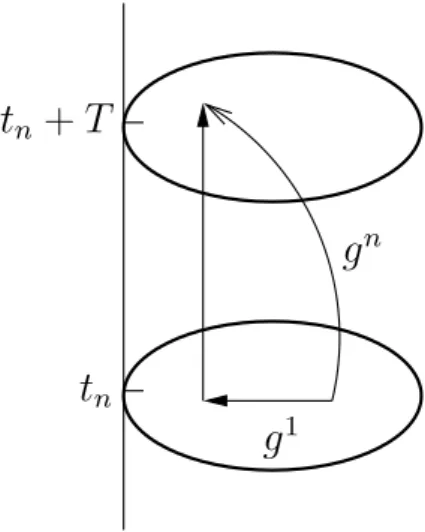
Consider the expanded phase space of the Hamiltonian system. Such a space has a natural structure of the bundle, the base of which is the discrete timetn=nT,n∈Z, and the fiber is the R×S space (Schutz, 1982). In this case, it is sufficient to describe the motion on some time inter-val (t0, t0+T ), for example, g1(ψ0, u0)=(ψ1, u1), where (ψ0, u0)is the initial state of the system, andg1is the map at one period (Arnold, 1989). In this way we have defined a map of the phase plane onto itself gn: R×S→R×S. The map is a diffeomorphism, which forms a one-parameter groupgn=(g1)nof diffeomorphisms of the phase plane, and preserves the phase volume. This statement follows from Li-ouville’s theorem. This bundle and the groupgnacting on it are shown in Fig. 1.
For the Hamiltonian (18) and its invariant of motion (25), this group can be written in the form of a set of nonlinear difference equations,
tn
g
ng
1tn
+
T
Fig. 1.Map at one period (after Arnold, 1988).
is known to be both ergodic and mixing (Arnold and Avez, 1968), and for many dynamical systems of interest, the phase variable randomizes much more rapidly than the action vari-ableu, allowing kinetic description in terms of a standard Fokker–Planck–Kolmogorov (FPK) equation for the distri-butionw(u)alone. For area-preserving maps, the distribution on any SA is trivially a constant. A common procedure for findingw(u)consists of iterating an initial state, or of solv-ing an FPK equation. Applysolv-ing the invariant distribution, we may replace time averages by phase-space averages in calcu-lating the steady state value of a physical observable. IfG(u) is an observable function in phase space, then the phase av-erage
hGi = Z
duw(u)G(u) (27)
is independent ofu0 (for almost all initial valuesu0in the
basin of a given SA). We are obliged to say strange attrac-tor; now we should wish to prove that these kinds of objects are common in the problem of interest, so we will try in the subsequent sections to develop all the proofs as explicitly as possible.
3 Dynamics of wave fields
We are going to inspect the problem of dynamics of parti-cles in space plasma wave fields. The first question of course is how to describe these wave fields. A common technique in studying the behavior of wave fields is to Fourier analyze transform into mode amplitudes, to obtain an equation of mo-tion for each mode. If only theN most important modes are kept, this motion is given by a set of ordinary differential equations describing the evolution in time of the mode am-plitude components. This procedure of Fourier analysis fol-lowed by truncation is called the Galerkin approximation. Any stationary nonlinear wave is known to be a strongly
exited state of a nonlinear medium, which emerges due to the competition between dispersion and nonlinearity. Such a wave represents in itself the bound state of a large number of harmonics. It is worthwhile emphasizing that these are not true modes of the nonlinear system, and thus interchange of energy among these quasimodes will occur even in the ab-sence of external noise. There exists a numberN that actu-ally truncates the wave spectrum exponentiactu-ally, and thisN is, in fact, the constant of coupling for stationary nonlinear waves (Sagdeev et al., 1988).
Another approach to describing wave fields consists of the proper choice of basis wave models in the standard form of nonlinear wave equations. For instance, the applicability of the Korteweg–de Vriez equation for describing nonlinear space plasma phenomena is well established. In that case, the nonlinear dispersion relation, which includes the main part of information about wave dynamics, is what we chiefly need (Bernstein et al., 1957; Lutomirski and Sudan, 1966). A gen-eral approach for deriving nonlinear dispersion relations has been developed in different techniques, by Whitham (1974), Karpman (1975), and Kaup and Newell (1978). They have shown that any nonlinear dispersion relation conserves its own form even if the wave propagates in a weakly inho-mogeneous and weakly nonstationary medium. This impor-tant conclusion follows from the strong stability of a non-linear wave packet. The basic model for modulated waves in a dispersive medium appears to be the familiar nonlinear Schrödinger (NLS) equation,
i ∂8/∂t+vg∂8/∂z+µ∂28/∂z2+ vg/2k0△⊥8 −g|82|8=0, (28) for the complex wave amplitude8(Karpman, 1975). Here the group velocityvgof the wave packet, and the parameters
of dispersionµand nonlinearitygare determined entirely by a nonlinear dispersion relationω=ω k2,|8|2in the usual way,
vg=(∂ω/∂k)k0, µ=
1 2 ∂vg/∂k
k0, g=
∂ω/∂|8|2
k0
.(29) The subscript denotes that we have to put these values at k=k0, wherek0is the characteristic wavenumber. The
interaction and compare obtained results with experimental data. We will rely on the data represented by the CLUS-TER mission (Santolik et al., 2003), which provided tem-porally high-resolution measurements of the wave events. In this work, chorus emissions have been measured at a radial distance of 4.4 Earth radii within a 2000 km region located close to the Equator. The wave vector direction in this re-gion is nearly parallel to the field lines, and the waveforms of the packet show a fine structure consisting of subpack-ets with amplitudes above 300 pT. In each wave packet, the frequency changes with a typical rate of a few kHz s−1, and
the spectrum is organized into two bands between 2 and 6 kHz. The spectral powerP of the wave has its peak value P ∼10−4nT2Hz−1 at the frequency 3.8 kHz, close to the
half-gyrofrequencyωB/2. The chorus emission, being a co-herent whistler mode, has a slowly varying amplitude (en-velope), with the time period T =200 ms determining the repetitive temporal structure of the chorus.
In order to interpret these results, we will use solutions of a nonlinear Schrödinger (NLS) equation, the applicability of which to whistler mode waves is well grounded (Karpman, 1975). In the wave frame, Eq. (28), for quasi-plane waves, takes the form
i8t+µ8zz−g|8|28=0, (30)
with 8=bexpiS, where b=Bw/B is the wave ampli-tude, normalized to the external magnetic fieldB, andS is the eikonal of the wave. It is known (Karpman, 1975) that an NLS equation has several different classes of solutions. Of these, the most stable solutions are the so-called two-parameter envelope solitons
b(z−vt )=asch(Qz−F t ) , (31)
a2=F2/G, (32)
F =Qv, G=ω0g, (33)
which are parameterized by the soliton velocityvand by the soliton spacescaleL=1/Q. We will assume the value ofv to be close tovg. These solutions describe a nonlinear wave
with a dispersion law
ω(k)=ω0(k)+ga2/2, (34)
whereω0(k)is the linear dispersion relation for whistlers ω0(k)=ωBk2c2/
ω2p+k2c2, (35)
andga2/2 is the nonlinear frequency shift. The NLS equa-tion is completely integrable and possesses an entire set of integrals of motion. One of them,
P =
Z
b2dt, (36)
is physically significant in virtue of the relation P =(1/2π )
Z
b2(ω)dω, (37)
which determines the spectral powerb2(ω)/(2π ). Substitut-ing Eq. (31) in the expression (36), we obtain
P =2a2/F =2F /G, (38)
and, a Fourier transform of Eq. (31) gives
b2(ω)/(2π )=(π P /4F )sch2(π ω/2F ) . (39) The spectral representation means that the nonlinear wave can be interpreted as a nonlinear wave packet whose ampli-tude and width1ω=4F /π, unlike a usual wave packet, are bound with the coupling. It is known that any spatially local-ized perturbations to an NLS equation will convert eventually into a set of solitons. This result has been proved by the tech-nique of inverse scattering transform (IST) (Newell, 1985). According to the IST, solitons of the NLS equations play the role of harmonic waves in linear systems, and the representa-tion of solurepresenta-tions in the form of a set of solitons corresponds to a Fourier transform in linear equations. So theN-soliton solution of the NLS equation is
b(z, t )= Ns X
i=1
aisch(Qiz−Fit ) , (40)
a2i =Fi2/G, (41)
whereNs determines the total number of solitons. The IST
involves quasi-classical quantization, and solutions (40) be-long to the discrete spectrum of values of a and F. The solitons of the NLS equation conserve physically significant properties, so the total spectral power is the sum of spectral powers of the single solitons,
P =X
i
Pi=21F /G, 1F = X
Fi, (42)
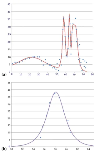
where1F is the half-width of a power spectrum. To inter-pret the spatio–temporal wave structure measured by Santo-lik et al. (2003), we apply the results of theoretical analy-sis to these data. We have approximated the temporal struc-ture of chorus presented by Santolik et al. (2003) in Fig. 2 by theN-soliton solution of the typeEw=P
(a)
(b)
Fig. 2. (a)Single wave packet with the envelope approximated by
N-soliton solution.(b)Smooth curve given by sch (t /1.18 ms) cor-responds to the 2th subpacket.
Indeed, it can be shown, any gradients of physical fields will lead to the change of wave vector:∂k/∂t= −∂ω/∂z. Con-sidering this expression and the nonlinear wave dispersion (34), we can obtain the equation of transfer of wave informa-tion
∂ ∂t+vg
∂ ∂z
ω=0. (43)
As a consequence, we conclude that the nonlinear dispersion relation is always the same along the group velocity vector, (∂t∂,vg∂z∂), even if the frequency (and wavenumber) changes
slowly over the time period of the wave, 2π/ω, such that ˙
ω2π/ω≪1ω˙=∂ω/∂t. (44)
Then taking into account the nonlinear wave dispersion (34), one computes the wave drift rate,ω˙ =(g/2)∂a2/∂t. Apply-ing to this the soliton-like solution for an envelope, the de-tailed evolution of the wave frequency (exponential growth of frequency on the initial stage, nonlinear dependence on the wave amplitude, etc.) can be studied. The mean and maximal rates are evaluated asω˙∼ga2/T ∼F2/(ωT ), andω˙max∼ ga2F /3∼F3/(3ω). One calculates F=pga2ω, with the
help of Eq. (41), then puts together the empiric data (Santolik et al., 2003); we evaluatega2/2∼200 Hz,F ∼1,2 kHz, and therefore, h ˙ωi ∼2 kHz s−1 and ω˙
max∼100 kHz s−1. Thus
we explicitly show that the condition (44) holds. Note that longitudinal inhomogeneities of the ambient magnetic field B(z)and particle densityNe(z)do not influence the effect
because the fundamental modeω0=ωBk2c2/ω2pis propor-tional to B/Ne, and this ratio is in fact a constant along a
force line near the equatorial plane. The rising tone of cho-rus is observed in the region of generation and formation of waveforms due to self-modulation and, due to the propaga-tion of waves away from this region when the modulapropaga-tion in-stability is stabilized, this effect may vanish, as was noted by Cully et al. (2008) and Wilson et al. (2011). The spectral gap is likely due to just the same competition between nonlin-earity and dispersion under conditions of the exact cyclotron and Landau resonance at ω=ωB/2, vr=vp. Presumably
the chirp-effect and spectral gap are rather the manifestation of intrinsic properties of the typical nonlinear whistler mode wave rather than a new type of emission.
The effect of diffraction on wave propagation is described by the third term of the NLS equation (28). Let AD be the angle of diffraction, AD=2/ kd, wheredis the perpendicu-lar size of the region of wave generation, andkis the wave number. In accordance with (Santolik et al., 2003), AD∼0.1 and these waves propagate from their source nearly paral-lel to the field line. Putting AD=0.1, k=0.25 km−1, we will have an estimate ofd,d∼100 km, and the lengthscale of the wave field,ld=kd2/2,ld≈2000 km, which is com-parable with the spacescale of the envelope. At z=0 the wave beam has a plane phase front and a Gaussian distri-bution of amplitudeb(r)=b(0)exp −r2/d2
. The solution of the equation shows that the width of the packet grows as d2(z)=d2 1+(z/ ld)2, and the radius of curvature grows as R=z+l2d/z. As z/ ld≫1; the originally plane wave becomes spherically divergent, its amplitude decreases as kd2b(0)/2z, and its width grows asd(z)≈2z/ kd. For ex-ample, if the wave was generated at a largeLand traveled a great distance to reach Polar, this effect will lead to a lower intensity at Polar (Tsurutani et al., 2011).
As noted above, the impact of the inhomogeneity of the ambient magnetic field and density fields on the wave prop-agation is negligible because of a constancy of the ratio B/Ne. The solutions of an NLS equation, in particular with
measurements (Hastings and Garrett, 1996). It is possible that it helps explain the modification of waveforms in wave events (Santolik et al., 2003).
Another powerful tool, especially when the explicit shape of a nonlinear wave is unknown, is spectral representation in the so-called form of time- and space-like wave packets (Sagdeev et al., 1988). Letf (t )be a periodic function,f (t+ T )=f (t ), given by the convergent Fourier series
f (t )=X n∈Z
fne−iωnt, ωn=2π n/T , (45) whose coefficientsfnsatisfy the Parceval identity,
X
n
|fn|2= hf2(t )i, hf2i = 1 2T
T Z
−T
f2(t )dt. (46)
Letf (t )correspond to a certain realization of a physical pro-cess. Then the measurable quantity ishf2i, and/or its spec-tral densityP
n|fn|2. One assumes this function character-izes the intensity of a nonlinear wave packet. As mentioned above, each packet is a bound state ofN quasimodes, and N takes part a constant of coupling. The implication of this is that as interchange of energy among these quasimodes occurs, the constant wave power, proportional tohf2i, will share evenly among the quasimodes. In virtue of Eq. (46), we obtainP
n|fn|2∼Nfr2∼const., and consequently,fr= f0/√N, where the value off0would have to be extracted
from a measured physical quantity, for instance, the spectral density. A more rigorous result, obtained in the theory of dis-tributions, states the following (Richtmyer, 1978). Letf (t ) be a generalized function such that
f (τ+1)=f (τ ), ei2π τf (τ )=f (τ ), τ=t /T , (47) then, this function is found to be
f (τ )=const.X n∈Z
δ(τ−n),const.=fr. (48)
The wide wavepacket approach follows from these state-ments and the physical meaning of the theory of nonlinear waves (Sagdeev et al., 1988). Taking the structure of a wide wave packet to be of the form
A (εt, εz)=X n
Ansin(nδkz−nδωt ) , (49)
where
δk=2π/L, δω=2π/T , (50)
L, T are the length and time scales of the problem. Then we suppose that all spectral characteristics An are equal-amplitude, and write the envelope of wave packet in the form A (εt, εz)=ArX
n
sin(nδkz−nδωt ) ,
Ar=A0/√N , N=1νT , (51)
whereA0is the characteristic amplitude of the wave, and1ν
is the width of the frequency spectrum. In the limitδk→0, expression (51) can be transformed into
A (εt, εz)=ArX n∈Z
δ(t /T−n). (52)
There is a time-like representation (TLR) of a wide wave packet. In deriving it we have used the relation
X
einx=2πXδ (x−2π n) , (53)
whereδ(·)is the Dirac delta function. Carrying out the same procedure with respect to Eq. (51), in another limitδω→ 0, the expression takes the form of a space-like (SL) wave packet
A (εt, εz)=ArX n∈Z
δ (z/L−n) . (54)
4 Whistler-electron interaction in the Earth’s radiation belts
of deterministic chaos, the statistical aspects of SAs have come under explicit study. The method has proved fruitful in describing the dynamics of electrons in the Earth and Jovian radiation belts.
4.1 Chaotic motion of the RB electrons driven by chorus
We are concerned with the dynamics of nonrelativistic elec-trons in the whistler mode chorus, which accelerates particles to relativistic energies through the resonance
−kz|vz| +ωB−ω=0. (55)
Taking into account the relationωBI=mvt2/2, we write the invariant of Hamiltonian flow (25) as
vt2=2(ωB/ω) vph(vr− |vz|) , (56) where vr=vph(ωB−ω) /ω is the resonance speed of an electron, and vt is the perpendicular (to B) velocity of an electron. Then the equations of motion (21)–(23) can be rep-resented in the form
˙ vt=
ω2B/2ωvph
b/√NTsinψX n∈Z
δ (t−nT ) ,
˙
ψ=ω (vt, ω)=ωB−ω−kzvr+
k2/2ωB
v2t. (57) We have also employed the invariant of motion, the value of the Bessel functionJ1′(0)=1/2 and the relationships
A/m=(ωB/ω) vphb, b=Bt/B. (58)
After integrating these equations, the problem is formulated in terms of aGn map, given by a closed pair of nonlinear difference equations,
Gn: ψun+1=un+Qsinψn,
n+1=ψn+14ωT u2n+1signu mod 2π, (59) where the new variableuand the control parameterQhave been introduced by the relations
u=vt/vr, Q=
ω2B/2ω√T P =ωBT ωB
2ω b
√
N, (60) andP is the wave power normalized toB2. The map (59) acts as the groupGn=(G1)n of diffeomorphisms of phase space, hence the pair(M, Gn), together with the invariant of motion is equivalent to the periodic flow (21)–(23). Khaz-anov et al. (2008a) and KhazKhaz-anov et al. (2011) have shown that the representation (52) is tantamount to that given by a solution of nonlinear wave Eq. (40). The physical expla-nation of this somewhat surprising result is quite clear. Any periodic, nonlinear wave can be described as wave packet consisting of some numberN of quasimodes with the fre-quency spacingδω∼1/T, whereT is the time period of the envelope. In the situation to which we refer, the half-width
1ν is about 1 kHz,T is no less than 100 ms, and therefore N∼1νT (∼102). On the other hand,1ν∼ω, which
indi-cates that 1/N∼ε, the small parameter given by Eq. (9). Thus we determine that the representation (52) is reasonable, so the results obtained in these approaches either coincide or differ only slightly.
To understand the physical nature of these results, we ex-amine the dynamics of a particle resonantly interacting with some quasimode of the wave packet. According to Eq. (57), the motion is governed by the pair of closed equations
˙ vt=
ωB2/2ωvph
b/√Nsinψ, ˙
ψ=k2/2ωB
vt2.
Settingvt =vc+1v, wherevcis the value ofvt in the reso-nance state, and linearizing this equation, we derive the equa-tions
¨
ψ+ω2bsinψ=0, ω2b=ωωBb/
√
N vc/2vp,
which describes the small (bounce) oscillations of the par-ticle with the frequencyωb. Now we apply the overlapping
criterion (Chirikov, 1979),ωb≥δω ∼T−1, to obtain the
condition of the onset of stochasticity, vc/vp≥(2ω/ωb)
√
N /bω2T2. (61)
Note that the criterion can be rewritten in the formTb≤T, where Tb
∼ω−b1 is the bounce period of the particle in the wave field. In amplitude–time terms, this relation deter-mines the condition for parametric resonance between the slow variations in the wave field and the proper oscillations of a particle in the field. Thus the basic resonances (55) and their interaction through parametric resonance play a crucial role in the appearance of stochastic motion.
Our interest now is to inspect the motion of relativistic electrons, driven by chorus. By integrating Eqs. (21)–(23) along with invariant of motion (25), we derive in the usual way thegnmap,
gn: un+1=un+Qsinψn,
ψn+1=ψn+(3/2)Ku−n+2/13signu mod 2π,
(62) written in the notations
pz/m=p, u=p3/2, andK=vgωBT . (63) Here the control parameterQis given by
Q=3 ωBvph/2ω1/2vgωB(P T )1/2,
P =b2/1ν, b=Bt/B. (64)
pair (M, gn), where M is a smooth manifold, and gn is a diffeomorphism. Denote by
J=∂ (un+1, ψn+1) ∂ (un, ψn)
(65) the Jacobi matrix of the map, the eigenvalues of which are given by the relations
detJ=λ1·λ2=1,
trJ=λ1+λ2=2+KQu−5/3, (66)
where detJ and trJ denote the determinant and the trace of the matrix, respectively. The Jacobian of (65) is equal to one, and therefore gn has the structure of a differentiable area-preserving map and(ψ, u)is the canonical pair of variables. It is known (Arnold and Avez, 1968) that the the geometri-cal structure ofM and dynamics ofgnonMare intimately closed, and that the condition
|trJ| =3 (67)
corresponds to a topological modification at which the dy-namics of the system becomes chaotic. In this situation, a sin-gle phase trajectory investigates all accessible phase space, which is called the strange attractor (SA). The strange attrac-tor is the invariant setgnSA=SA, n→ ∞ tightly embed-ded in phase space. The motion on any SA is random over a wide range ofQdue to the global stability of the SA, on which all means (observables) are stable indifferent of any (reasonable) initial conditions. Then we apply the condition of Eq. (67) to the relation (66) to obtain the upper bound of {u}
ub=(KQ)3/5. (68)
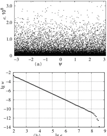
Shown in Fig. 3 is the strange attractor of the pair(M, gn). Figure 3 shows that the stochastic region extends to the val-ues ofupredicted by Eq. (68).
Finally, using the relations (63) and (68) along with invari-ant of motion (25), we find theQdependence of the upper boundary of energy spectrumEb,
Eb=m(KQ)2/5. (69)
At typical values of parameters,ωB/ω=2, ωB/2π=8× 103Hz, P =10−4nT2Hz−1, B=300 nT, T =2×10⁻¹s
(Santolik et al., 2003), the expression (69) yields Eb≃
8 MeV. In this way as above, we can say the same about the pair(M, Gn), just changing the order of words a little. In-deed, in this case, the condition (67) proves to determine the lower bound of{u},
uc=4/ωB2T √
P T , (70)
which is in good agreement with the numerical solutions and results of qualitative analysis. With the values of the parame-ters as given above, the expression (70) yieldsuc≈1×10⁻³.
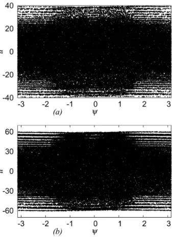
Fig. 3.Phase space for the mapgn after 2×10⁶ iterations with
(a)Q=0.5 and(b)Q=0.98.
The phase space of the mapGnis shown in Fig. 4. The over-all picture of the phase space is quite different for u < uc
andu > uc. In the first case, the motion is regular. Figure 4
indicates the existence of a threshold for the initial particle velocity above which the trajectory becomes chaotic. We as-sume that nonlinear electron acceleration by a wave packet of whistler mode waves is always a stochastic process.
Now using the invariant of motion (56) and resonance con-dition (55), we have the relationship
e=1+u2/42, (71)
wheree=E/Eris the particle energy normalized to that at
exact resonance (Er≃25 keV). Putting in the expression (71) u=ucandu0=√2ωB/ω, we determine the range of heat-inge∈(ec, e0), where
ec≃1+u2c/2, e0=(1+ωB/2ω)2, (72) and evaluate (72) asEc∼25 keV,E0∼100 keV. Lastly, the
expression (72) is taken as a criterion that stochastic motion occurs, making available reliable information about the in-tensity of wave fields. SettingucbevT/vr, wherevTis the
0 0.01 0.02
−3 −2 −1 0 1 2 3
u
ψ
(b)
Fig. 4.Phase space for the mapGn atQ=2×10⁻³.(a)A
sin-gle trajectory of length 2×10⁵. The initial point (10−4, 3×10⁻¹). (b)A single trajectory of length 8×10³. The initial point (10−4, 10−5).
u2c≪1, we evaluate the available wave intensity,
Pth≥10−8nT2Hz−1, Bth≥1 pT. (73)
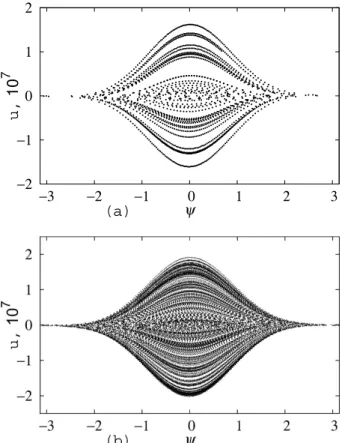
The equations from which the SA arises are usually parame-terized by some control parameter, whose variation changes the character of the dynamics. The control parameter Q, as a rule, depends directly on the intensity of the wave field. First, we consider the dynamics of gn under condi-tions when the wave perturbation is larger than that observed. Figure 5 shows the evolution of the system over time at Q=5×10⁵. The picture indicates that the system
demon-strates both chaotic and regular dynamics, a so-called chaotic intermittent behavior. This behavior is more complex, ex-hibiting random transitions between regular and stochastic motion. In this regime, stochastic diffusion governed by the SA is realized through the drift of orbits in phase space and can be expressed in terms of a FPK equation that describes an increment in entropy rather than the diffusion in action (Khazanov et al., 2008b). The phase modification is associ-ated with the appearance of fixed elliptic points, which occur when an initial saddle point of the attractor changes to a sta-ble elliptic point as the control parameterQincreases above the appropriate critical value,Qc. To determine these points,
−2 −1 0 1 2
−3 −2 −1 0 1 2 3
u,
10
7
ψ
(a)
Fig. 5.Intermittent chaotic behavior of map (62) withQ=5×10⁵.
(a)t=2×10³and(b)t=2·104iterations of a single initial con-dition.
we write sinψ0=0,
3K/2u20/3=2π, u0=ub, (74)
whereub is given by expression (68). These equations are
satisfied providedQtakes the value
Q=Qc, Qc=(3K/4π )5/2K−1. (75)
The test does predict the phase modification rather well. We find this behavior numerically and can give an interpretation in terms of the theory developed by Khazanov et al. (2008b). SubstitutingQcin Eqs. (69) and (74), we obtainu0≃3×10³,
and thereforeE0≃100 MeV. Finally, Eq. (75) yieldsQc≃
103, which is three orders of magnitude larger than typical values ofQ(∼0.5−1). The explicit expression forPc, the
value of the wave power at which pronounced intermittent dynamics occur, results immediately from Eq. (64):
Pc=(2/9)(3/4π )5(ωT )2(B2/ω), Pc∼103nT2Hz−1. (76)
The results show that the intermittent chaotic motion is possi-ble only in extremely strong (Bw/B∼1) wave fields. Under
4.2 Statistical properties of the dynamics
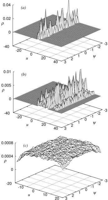
The dynamics of the system exhibits a random walk, and all points of the phase trajectory tend to a certain strange at-tractor (SA) atn→ ∞. The appearance of such an SA repre-sents persistent chaotic motion over a global domain of phase space, as shown in Fig. 6. There the joint probability density ρ(ψ, u, t )is proportional to the number of phase points in the element of phase space. We see that after a few iterations the action distribution remains localized while phase randomiza-tion occurs, and that the final distriburandomiza-tion is random. Thus, we have good evidence for statistical properties in the re-gion for which the system exhibits chaotic motion. Once the phase variable becomes rapidly varying, the evolution of the coarse-graining function
w(u, t )= 1 2π
π Z
−π
ρ (ψ, u, t ) dψ, (77)
obeys the Fokker–Planck–Kolmogorov (FPK) equation for theuvariable alone. In this case, the nature of the evolution to the steady state is so-called deterministic diffusion (Licht-enberg and Lieberman, 1992). As the canonical status of the phase variables has been demonstrated above, the distribu-tion funcdistribu-tion (probability density)w(u;t )is governed by the FPK equation in the standard form
∂w(u;t )
∂t =
1 2
∂ ∂uD
∂w
∂u. (78)
Here D is the conventional diffusion coefficient in phase space,
D=< (un+1−un)2> T−1=Q2/2T , (79) where(un+1−un)is substituted from eithergnorGn,<·> denotes the phase average, andT is the timescale of the prob-lem. The function w(u, t )is a differentiable function sup-ported in{U}with the norming
Z
u∈{U}
w(u, t )du=1, (80)
where{U}is a range of the variableu.
First, by means ofgn (or Gn) we calculate the diffusion coefficient and evaluate the characteristic time for redistribu-tion ofuover the spectrum
td≃2u2m/D=T (2um/Q)2. (81)
We exploit the FPK equation with w(u)and its derivative ∂w/∂uvanishing at the upper and lower boundaries. We in-troduce the moment< u2>=Rπ
−πduu2w(u), multiply equa-tion (78) byu2, and integrate the resulting equation overuto obtain
d< u2> /dt=D, u∈ {U|u≤um}. (82)
(a)
-3 -2 -1 0 1 2 3
ψ -40
-20 0
20 40 u
0 0.02 0.04
ρ
(b)
-3 -2 -1 0 1 2 3
ψ -40
-20 0
20 40 u
0 0.005 0.01
ρ
(c)
-3 -2 -1 0 1 2 3
ψ -20
-10 0
10 20 u
0 0.0004 0.0008
ρ
Fig. 6. Joint distributionρ(ψ, u)computed numerically viagn at
several different numbers of steps:(a)102,(b)103, and(c)2×10⁶. The parameters are the same as in Fig. 3a.
The restriction on u is needed because the spectrum is bounded from above. Then, by means of Eq. (60) along with Eq. (72), we calculate by formulas (79) and (81) the diffu-sion coefficient Du≈1 s−1 and the time of diffusion inu, td∼16 s. For the functionw(u)restricted to[uc, u0], the
in-variant distribution can be given by
w(u)=(u0−uc)−1. (83)
This means that the random variableuis evenly distributed on[uc, u0]. Now we evaluate the energy distribution
func-tion,w(ε), in the range of non-relativistic energies. Consid-ering u2=4 √e−1
transformation w(e)de=w(u)du determines this problem completely, subject to appropriate boundary conditions. The corresponding solution forw(e)is found to be
w(e)=w(u)/2
e √e−11/2, e∈(ec, e0). (84)
By means of Eq. (84) we find the mean energyhei ∼0.5e0.
This solution relates directly to the behavior of the system near the order–chaos bifurcation transition. Equation (82) may be written as
d< vt2> /dt=Duvr2. (85)
Then considering Eq. (85) we find the rate of change of magnetic moment µ, µ˙ =vr2Du/2B, and the heating rate
˙
E≃E0/td ∼6 keV s−1. This result is nontrivial, because chaotic motion in the (u, ψ)-phase space leads to nonadi-abatic magnetic moment changes and stochastic heating of plasma particles. The gyroradius is a direct measure of the perpendicular electron velocity. Thus the stochastic heating will be accompanied by a radial drift of particles in space. Indeed, considering the relationr=vt/ωB, via (85), we get the following expression
d< r2>
dt =Dt, Dt=Duv 2 t/ω2B,
∼1010cm2s−1 ,
whereDt is the coefficient of collisionless diffusion across the ambient magnetic field.
Now we describe the effects associated with stochastic heating of high-energy particles. Due to one-to-one corre-spondence, u=p3/2, and using dp=2du/3p1/2, one ob-tains the coefficient of diffusion inp,Dp=4Du/9p. Then the measure-preserving transformationwp=wu|∂u/∂p| re-sults in the probability density inp,wp=3√p/2p3b/2. There is an important relationship,w2pDp=wu2Du. Furthermore, one can easily prove the invariant relation
w2vDv=w2uDu=inv.,inv.=1/2td (86) takes place for anyv(u), and depends smoothly onu, the co-ordinate on the SA, whose distribution functionwv=w(v) relates with wu through a measure-preserving transforma-tion, withDvgiven by a quadratic form of its variation. We see that the invariant is given by the rate of diffusion on the SA. We come to know as well that the FPK equation for w(v, t )can be written in divergent form
∂w(v, t )
∂t =
∂
∂vJ (v), J (v)= 1 2
Dv
∂ ∂v+dv
w(v, t ), (87) where the transport coefficients are given by
Dv=Du(∂v/∂u)2, dv= 1
2Du∂/∂v (∂v/∂u)
2. (88)
The above equations have important consequences in de-termining the heating rate. Then, introducing the particle
energy distribution w(e, t ), and taking into account the invariant of motion and the relation e=E/m and E= q
m2+pz2+2mωBI, we find, after appropriate transforma-tions, that the following equation forw(e, t )results in
∂w(e, t )
∂t =
∂
∂eJ (e), J (e)= Du
2
4
9e ∂ ∂e−
2 9e2
w(e, t ). (89) Then it may be possible to find the heating rate
dE dt ≃
8 9
eb e
2 ·Eb
td , td=
4eb3 Q2 !
T , (90)
wheretd is the relaxation time to the steady-state distribu-tion. It is worth noting that the injection mechanism at low energies, which may be intimately related to particle heating is the important aspect of space physics. Since the rate of electron cyclotron resonance heating is proportional toE−2 this is, indeed the case. We put the characteristic values of these quantities at typical conditions,ωB/ω=2,ωB/2π= 8×10³Hz,P =10−4nT2Hz−1,B=300 nT,T =2×10⁻¹s,
to determine, with the help of Eqs. (69) and (90), the upper boundary energy spectrum Eb≈8 MeV, the time of
diffu-siontd≈2×10³s, and the heating rateE˙≈4 keV s−1, which are all in reasonable agreement with experimental data (Se-lesnick et al., 1997; Se(Se-lesnick, 2006). These results lead to two important observations:
1. Nonlinear electron acceleration by a whistler wave is always a stochastic process when the wave power of the wave exceeds the threshold value given by Eq. (73).
2. In this case the related quantities have the following dependencies on the wave power,
Eb∝P1/5, td∝P−2/5,E˙∝P3/5, (91) with the power law indices determined by the type of nonlinearity in the phase advance equation.
4.3 Adaptability of the Fokker–Planck–Kolmogorov equation
We have seen that diffusion on a strange attractor (SA) is described by a Fokker–Planck–Kolmogorov (FPK) equa-tion for theu variable alone, where u is a canonical vari-able on the SA, proper for a certain physical situation. The FPK equation to which we refer indicates that an initialδ function distribution diffuses to a random distribution. Any measure-preserving transformation fromuto some new vari-ablev(u)has been shown to preserve the invariant relation w2(u)D(u)=1/2td, with u replaced by v, indicating the universal nature of the diffusion process on any SA. In this case, the distributionf (v)can be found by a direct transfor-mationf (v)=f (u)du/dv without solving a relative FPK equation. However, if we are, for example, concerned with the evolution of the energy spectrum, we should use the FPK in divergent form.
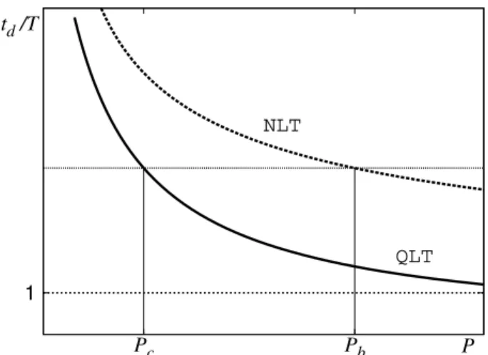
Quasi-linear theory (QLT) does predict the long-time evo-lution of RB electrons on the basis of an FPK equation. However, in the standard formulation (Lyons and Williams, 1984; Summers et al., 2007), the wave field of whistlers is treated as random, broadband and phase-incoherent. Thus, this formalism can not be directly applied to the problem of electron motion in the regular wave field of chorus. In the nonlinear approach, we apply just the same FPK equation in which phase averaging is made due to dynamics itself, and all time means of observable functions are equal to the phase space means. This approach corresponds to the stan-dard FPK description in statistical mechanics and facilitates the applicability of kinetic models in which the RB dynam-ics is simulated (Khazanov, 2011). As it is known, QLTs are based on some linearized equations of motion, and the char-acteristic time of diffusion in energy is given bytd=E2/D that depends on the wave powerP as P−1 in certain en-ergy ranges. In the nonlinear theory (NLT), the rate of dif-fusion hinges on the type of interaction, for instance, it obeys the scaling td∼P−2/5 for chorus-RB electron interaction. Shown in Fig. 7 is the time of diffusion as a function of wave power. Since the inequalitytd/T ≫1 is a condition for ap-plying the FPK description, these dependencies have impor-tant consequences in determining the range of values of wave power for which the FPK formalism is valid. It is just the same thing to evaluate the permissible values of chorus wave fields, P1,P2 and susceptible to FPK description, in QLT
and NLT, respectively. Here,P1 andP2 are determined by
Eqs. (73) and (76), respectively. They yieldP1/P0=10−4,
andP2/P0=107, whereP0=10−4nT2Hz−1 is the typical
value of wave power (Santolik et al., 2003).
Although it is normally thought that the results from sim-ple problems give qualitative predictions of the behavior of more complicated physical systems, many questions con-cerning the dynamics of the system still exist. A particularly interesting aspect concerns the effects resulting from the res-onance interaction with the quasi-coherent whistler waves.
1
Pc Pb
td /T
P
QLT NLT
Fig. 7.Time of diffusion as a function of wave power. HereP1and
P2 are the critical wave powers for the applicability of the FPK equation in QLT and NLT, respectively.
The effect of a magnetic mirror in modifying the motion can also play an essential role in certain physical situations.
Such a physical situation can emerge when RB electrons interact with the so-called quasi-coherent chorus, whose fre-quency spectrum contains low-intensity isotropic white noise (Tsurutani et al., 2011). The physical explanation for these wave events is quite clear. These are likely to relate to the irregular nature of the Earth’s ring current injections, which generate chorus (Liemohn, 2006).
The level of background noise is relatively small; conse-quently, this effect can exhibit in the equations of motion only as the fluctuations of parametersωB andQ. Thus the control parameter is a function of the magnitude of wave fieldb, and thereforeQ→Q(1+ξ ),ωB→ωB(1+ξ ). Here, ξ=δb/bis the random variable having a Gaussian probabil-ity densprobabil-ity
p(ξ )=√1 2π σ exp
−ξ2/2σ2,
the mean-square value of which is hξnξn′i =σ2δnn′, where σ2is the intensity of noise, andδis the Kronecker delta.
In order to understand how the extrinsic noise modifies dynamics, we consider its influence on motion separately. Thus, we include the additional noise in Gn only in the phase advance equation, to obtain the closed pair of nonlin-ear stochastic equations
un+1=un+Qsinψn,
ψn+1=ψn+ξn+(1/4)ωT u2n+1 mod 2π, (92)
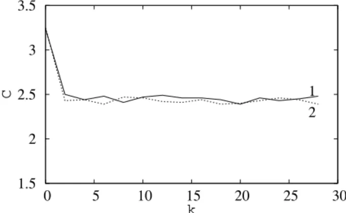
where the termξnplays the role of a weak stochastic force. Numeral investigation of a related quantity, the correlation functionC(k),
C(k)=(1/N )X n∈N
wherek is the step lag, gives the results shown in Fig. 8. The motion has been shown to beδ-correlated, withC(k)=0 fork6=0; this represents a very strong chaotic property, i.e., a complete decorrelation of the motion in one mapping pe-riod. Note that FPK description is valid only when the func-tionC(k) falls off rapidly with the number of mapping it-erations. The effect of extrinsic noise manifests itself in the FPK equation as an additional term in the coefficient of dif-fusion,D/Du=1σ2/Q2. This effect does not significantly affect diffusion induced by stochasticity, due to the global stability of the SA.
The situation is quite different for ion cyclotron resonance heating (ICRH) (Lichtenberg and Lieberman, 1992). In this case the dynamics is intrinsically degenerate, and the non-linearity arises from the finite gyroradius, which leads to a spectrum of modes in the motion, and the term proportional toQoccurs in the phase advance equation. This method has been used by the authors in conjunction with the problem of ICRH at the front of a shock (Khazanov et al., 2010).
Now we want to study how the Earth’s magnetic mirror effects change the dynamics ofGn and how much impact it has on the statistical properties and long-term evolution of the system.
The drift equations for particle motion in a current-free field are given by Schmidt (1979):
vd=vkB/B+[F,B]/B2, F= −
µ+mvk2/B,
dvk/dt= −(µ/m) ∂B/∂s, (93)
wherevdis the drift velocity,F the free force averaged over a gyro-orbit,µthe magnetic moment, ands the coordinate along the field line.
In the drift approximation, µ is an adiabatic invariant, which is assumed to be well conserved. Since the energy of a charged particle gyrating in the Earth’s magnetic mir-ror is strictly conserved,vkis related to the constants of the motionµandEthrough the relationvk=√2(E−µB)/m, which is easily calculated for a given function B. In the equations of motion, describing the resonant interaction with high-frequency wave fields, the forces given by Eq. (93) aver-age to zero, as do all other off-resonant terms. All the same, residual effects are always present, which lead to the usual distortions of the phase plane near resonances of the princi-pal frequencies, and can be physically associated with the loss of phase coherence from one passage along the field line. To show how this occurs, we first write Eq. (10) as y=yd+rcosθ, whereyd is the guiding center position of the gyrating particle. Then, this dependence in theψ vari-able gives rise to the termktyd, and as a consequence, the term{ktvdT}n−{ktvdT}n+1= {ktvdT}, where{·}is the
frac-tional part, occurs in the phase advance equation. We can eliminate this term by a shift ofzort; however, small asym-metries or time variations in the magnetic field exist, which allow stochastic diffusion to occur. If these variations are ran-dom, we would write an independent equation{ktvdT} =ξn,
1.5 2 2.5 3 3.5
0 5 10 15 20 25 30
C
k
1
2
Fig. 8.Dependence of the correlation functionC(k)onk,
corre-sponding (1) to the mapGnwithout noise and (2) with noise (92) for calculations over 2000 points.
whereξnis a random variable. At last, assuming that these fluctuations are white noise, we arrive at equations of motion that are similar to the map (92). Hence, the system generates diffusion analogous to that described above. Some numerical experiments seem to verify that behavior (Faith et al., 1997; Roth et al., 1999; Zheng et al., 2012, 2013). It is obvious that the effect of bouncing on the dynamics may be investigated in just the same way.
It should be noted that the termξnin the system acts with-out significantly changing its statistical properties; moreover, numerical investigations obviously reveal that the SA re-mains in the sense such that we can’t tell the SA ofGnfrom that of system (92) by whichever sign. However, if we re-move the nonlinear term from the phase advance equation, then the term dominates the behavior of the system fully.
Now, we examine the problem of energization of RB electrons subject to resonant coupling with oblique large-amplitude whistler waves. The existence of such waves is confirmed by direct measurements (Cattell et al., 2008; Cully et al., 2008; Kellogg et al., 2011; Kersten et al., 2011; Wil-son et al., 2011). In our calculation, we will rely on the rel-evant experimental data of Cattell et al. (2008) and Wilson et al. (2011). These waves have a broad range of wave nor-mal anglesϑwith respect to the magnetic field (20–60◦) and large peak-to-peak amplitudes El∼(100−200)mV m−1
withBt∼1 nT,Et∼100 mV m−1. The timescale of the en-velope is typically T ∼0.2 s, and the mean value of the frequency at peak wave power is (0.2–0.25)ωB(∼1.5 kHz). We have used this data, as well as the dispersion relation ω=ωB
k2/ω2pcosϑ (Stix, 1992) where ωp is the
elec-tron plasma frequency (∼1.1×10⁵s−1), to estimate the
wavenumberk∼2×10⁻⁴m−1and group velocityv g∼5×
107m s−1.
Fourier amplitudes. Thus we will examine only the resonance of driving with the fundamental of gyromotion, kzpz/E+ ωBm/E−ω=0. Then, because the Bessel functions tend to zero as 1/√ktratktr→ ∞, we have to choosektr≈1−3, which corresponds to the values ofJ1(·)near a maximum
in the Bessel function. This choice automatically imposes certain restrictions on the energy spectrum of particles. In-deed, taking into account the invariant of motion (25), and the relationsktr∼(1−3),ωB/ kz∼1,r=
√
2mωBI /mωB, we find, without much difficulty, the range of particle ener-gies, in which the wave-particle interaction is most effective, (kt/ kz)√2E/m∼(1−3),E <10 MeV.
First we will study the problem provided the condi-tion Bt/B≫ J1(·)U0/J1′m
√
E/m holds. By integrating Eqs. (21)–(23) along with invariant of motion (25), we de-rive, in the usual way, a map that is similar to thegnmap de-scribing the chorus–electron interaction, except that the con-trol parameter contains the termJ1′(ktr)(∼0.1). This simi-larity means that the given dynamical system manifests it-self in just the same way as thegn map; as a consequence, the heating rate is governed by the same Eq. (90). However, the intensity of coupling, in this case, is determined by the magnitude of the wave field multiplied by the factorJ1′(·). It stands to reason that the expression (91) remains the same, after appropriate modifications, √P →√P J1′(·). So these waves are about four times larger in magnitude than those measured by SAMPEX (The Solar Anomalous and Magneto-spheric Particle Explorer), and the heating rate of the process is comparable to that caused by chorus–electron coupling.
Let the dynamics be dominated by interaction of the parti-cle with the electrostatic (ES) component of a wave. Taking the wave field to be in the form of a space-like (SL) wave packet (54), we convert the equations of motion into the map, un+1=un+Qsinψn, ψn+1=ψn+1/un+1, mod 2π, (94) where the variableuand the control parameterQare defined by the relations,
u=(E/mωT ) , Q=J1(·)U0/m √
N , (95)
and the spectral characteristic N and the ES potential are given by
N=1νT , U0=E0l/ kz. (96)
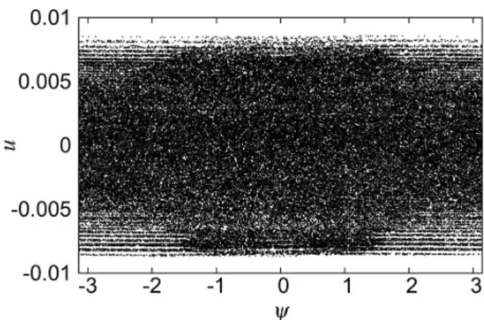
The map (94) belongs to the class of Fermi mappings, there-fore this map possesses an SA (Lichtenberg and Lieberman, 1992). Shown in Fig. 9 is the SA of the system, whose upper bound is defined by the equations
ub=pQ, Eb=ωTpQm, (97)
which is borne out numerically.
The invariant distribution on the SA is a trivial constant, and the time of diffusion in energy is found to be
td=(4/Q)T . (98)
Fig. 9.Phase spaceu−ψfor the map (94) atQ=0.98×10⁻⁴.
We see the extent and rate of heating at this wave-particle in-teraction are proportional toU0J1(ktr), just as it is expected. We extract from Eqs. (94) and (98) the following estimates of Eb≃5 MeV andtd≃104s. We have seen that generic,
non-linear behavior in the interaction with oblique waves restrict the extent and rate of particle heating, which, to a certain ex-tent, accounts for the nature of wave-particle interaction.
Electron acceleration in the radiation belts is a well-established fact. Whistler-RB electron coupling ranks among the most important accelerate mechanisms that are likely to play a major role in maintaining the entire pool of RB elec-trons. Acceleration of RB electrons, which are driven by whistlers up to relativistic energies, can proceed in the very short time of∼1 h or less, and manifest itself in bursty rela-tivistic electron precipitation events. We have used topolog-ical arguments to determine the value of the control param-eter at which the dynamical system exhibits chaotic motion, in the form of a strange attractor. In this case, every particle can explore the entire phase space energetically accessible to it; as a result, the upper bound of the strange attractor can be put on a one-to-one correspondence with the upper boundary of an energy spectrum whose value depends parametrically on the spectral power of the wave. The chaotic motion on the strange attractor is ergodic with mixing, and as a con-sequence the evolution of the distribution function and all means obeys a FPK equation.
5 Stochastic acceleration of cosmic-ray electrons
It is well known that high-energy particles observed in cos-mic rays can be regarded as tails of the particle distribution in space plasmas. The energy relation (the energy per unit volume of space plasma is approximately equal to the energy per unit volume of cosmic rays) shows that collective pro-cesses occurring in the plasma can play an important role in the evolution of the energy spectra of cosmic rays. In this connection, it becomes relevant to determine how the en-ergy should be redistributed in cosmic rays so that the enen-ergy spectra could contain particles with very high energies (Ka-plan and Tsytovich, 1973; Ginzburg, 1989). Supernova rem-nant shocks are thought to be the primary source of cosmic rays, because supernova remnants (SNRs) are able to pro-vide the energy necessary to maintain the observed cosmic ray density. Synchrotron emission from SNRs indicates the presence of 100 TeV electrons, and inverse Compton scat-tering of background photons by ultrarelativistic (UR) elec-trons is a very plausible explanation for TeVγ-ray emission from young SNRs (Reynolds, 2001; Treumann and Tera-sawa, 2001; Vink, 2004; Abdo et al., 2009).
The current description of cosmic ray acceleration up to UR energies is the well-known first-order Fermi acceleration at the SNR shock front (Bell, 1978; Blandford and Ostriker, 1978). In the first-order Fermi model, wave turbulence makes the particle momenta isotropic, thus particles can cross the shock front many times. Simulations show that the efficiency of the mechanism depends on the spectra and amplitudes of MHD fluctuations, and their fluctuation amplitudes, and rel-ativistic particle distributions are a natural consequence of the stochastic acceleration by turbulent plasma waves. As the effect of energy loss through synchrotron emission is not included in the model, the gradual high-energy cutoff has been attributed to the balance between the acceleration and escape processes, which leads to a steady-state distribution (Liu et al., 2008; Muranushi and Inutsuka, 2009). In addition to this, it should be noted, the wave-particle interactions in the model are treated in the linear approximation.
There is also another treatment of the problem relating Hamiltonian chaos to nonlinear interactions of particles with plasma waves (Sagdeev et al., 1988; Horton and Ichikawa, 1996). A dynamical system that can be represented by a measure-preserving map and that illustrates the nature of stochasticity was proposed by Fermi as a model for cos-mic ray acceleration. There are, as a matter of fact, vari-ous versions of this model, all characterized by a phase ad-vance equation that is inversely proportional to the velocity. The review of the class of Fermi maps was made by Licht-enberg and Lieberman (1992). Another important model is the relativistic standard map (RSM), which was indepen-dently proposed by Chernikov et al. (1989) and Nomura et al. (1992). The RSM is the relativistic generalization of the stan-dard map (SM), introduced by Chirikov (1979). The stanstan-dard map is well known for application to a wide class of
prob-lems, including the confinement of particles in fusion de-vices, radio-frequency heating, acceleration, and heating of particles by nonlinear wave packets (Lichtenberg and Lieber-man, 1992). Thus, it was natural to study in terms of the RSM how relativistic effects modify the nonlinear motion described by the SM. It is worth noting that these investi-gations of RSM provide us with a more profound knowl-edge of many general properties of relativistic chaotic sys-tems. A possible mechanism for strong heating was proposed by Papadopoulos, and the first simulation was performed by Cargill and Papadopoulos (1988). It was shown that colli-sionless shock waves propagating away from a supernova may be directly responsible for the 10 keV X-ray emission seen in SNRs. A sequence of plasma instabilities between the reflected ions and the background electrons at the foot of the shock front can give rise to rapid anomalous heating of electrons. A somewhat different approach to the problem was taken by Dieckmann et al. (2004). A self-consistent sim-ulation was performed by these authors to show that ions reflected from SNR shocks can excite large-amplitude elec-trostatic waves through the beam-plasma instability. Another mechanism that has been investigated to explain the accel-eration process includes the nonlinear coupling of the beam of cosmic rays escaping away from a supernova, with back-ground Langmuir waves. Estimates of the rate of instability from this type of interaction were made by Ginzburg (1989), who found that the characteristic time of the instability would be about a few years.
As a consequence of this, chaotic dynamics of relativistic electrons is of particular interest. Thus, the nonlinear inter-action of high-energy electrons with an extraordinary elec-tromagnetic wave propagating across a given magnetic field was investigated by Zaslavsky et al. (1987). They estimated the rate of the diffusion and found it to be sufficient to ac-celerate an electron up to UR energies. Chaotic dynamics of relativistic electrons in the spectrum of Langmuir waves has been considered by Klimov and Tel’nikhin (1995) in terms of a map given by the closed pair of nonlinear difference equations. More complete calculations, including the gy-roresonance effect were made by Nagornykh and Tel’nikhin (2003) who showed the role of the gyromotion in random-izing the phase of particles. Finally, Krotov and Tel’nikhin (1998) have shown that the stochastic heating of particles by the nonlinear Langmuir wave packet in space plasmas can be regarded as a possible mechanism for the formation of the energy spectrum of cosmic rays.
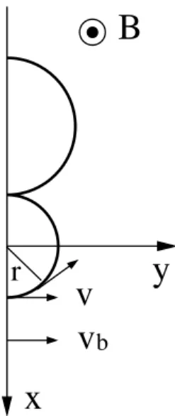
5.1 Stochastic surfing electron acceleration at Galactic shocks
corresponds to the empiric spectrum. However, this spectrum of escaping relativistic ions turns out to be unstable in regard to some plasma instabilities. The self-consistent simulation of Dieckmann et al. (2004) showed that such a beam of rel-ativistic ions can induce a collisionless shock. This shock arises as a consequence of strong nonlinear upper-hybrid (UH) solitary waves which are driven via the beam instabil-ity by the ion beam. In this scenario, typical for collision-less shock generation (Artsimovich and Sagdeev, 1979), the shock front is formed by the dissipative process caused by particle heating, and the tail of the wave manifests itself as UH wave perturbations in the foot of the quasi-perpendicular shock. The dispersion law of the electrostatic UH wave (its wave potential is about 1 mc2) at the foot of shock front is ω=kvf, vf≤vb, ω=
q
ω2B+ωp2, (99)
the dispersion law of which is a typical condition for plasma modes induced by a beam (Artsimovich and Sagdeev, 1979), whereωp is the electron plasma frequency, and vf,vb are
the speed of the front and beam respectively. In this situa-tion electrons can be accelerated up to relativistic energies through the mechanism of surfing (Sagdeev et al., 1988). The model of surfing is in general similar to the Fermi–Ulam model (Lichtenberg and Lieberman, 1992) of acceleration in which the fixed wall plays the role of Lorentz force. This force doesn’t change the particle energy and results only in the drift of particles along the front (look at the picture in Fig. 10). The way the electrons gain energy is by picking up wave field energy in multiple encounters with the shock front (Sagdeev et al., 1988).
Taking the original potential of the wave to be of the form
ϕ(y, t )=ϕ0cos(ky−ωt ) , (100)
then Eq. (22) can be written as ˙
I =X
n
ϕ0nJn(kr)sin(nθ−ωt ) , θ˙=ωBm/E, (101)
E=pm2+2mωBI , ψ=nθ−ωt. (102)
In this case electron cyclotron resonance heating (ECRH) is accomplished by resonance between the gyrofrequency and the UH wave,
˙
ψ=sωBm/Er−ω=0, s∈Zs⊂Z, (103)
which is satisfied for a series ofs-values for particles of dif-ferent energies.
To begin with, let us consider the dynamics in a single mode. Choosing a particle resonance s=l, we can write Eqs. (101)–(102) as
˙
I=ϕ0lJl(kr)sin(ψ ), ψ˙ =lωBm/E−ω. (104) Linearizing with Eqs. (104) in the vicinity of the exact res-onance, putting of quantities at the resres-onance, we obtain the
y
x
r
v
B
v
b
Fig. 10.Particle trajectory at the front of a shock.
equation of phase oscillations
¨
ψ+ωb2sinψ=0, ωb=ωB e
s ω
ωB 5/3
e2/3U0,
e=E/m, U0=ϕ0/m, (105)
whereωbis the bounce frequency in the wave field. In
writ-ing (105) we have taken advantage of the dispersion law (99), the relation (kr)r=l, and used the asymptotic expression of
the Bessel functionJl(l)≈1/ l1/3, which is valid forl≫1. By requiringωb≥δω, whereδω=ωB/eis the spacing be-tween adjacent modes, we obtain the overlap condition ec≥(ωB/ω)5/3/U03/2, (106) which indicates the value of wave field at which electrons with energyecan be accelerated in random manner. At last, we find from above the characteristic time of the variation of I and ψ is of order 2π/ωb∼(2π/ωB) e, which essen-tially exceeds one period 2π/ω. The small parameter ε= ωB/ωe≈1/sserves as the condition for the applicability of the adiabatic approach, developed by the authors (Khazanov et al., 2010).
The condition of adiabaticity,ψ˙ ≪ωψ,I˙≪ωIallows us to write Eqs. (101)–(102) in the form
˙
ψ=sωBe−1−ω,I˙=2sJs(s)ϕ0sinψ T X
δ (t−nT ) ,
T =2π e/ωB. (107)
We have carried out the following transformation here,
X
ϕ0nJn(·)einθ−iωt=ϕ0sJs(s)eisθ−iωt X
n6=s
einωBt /e,
employed the identity P
einωBt /e=TP