www.nonlin-processes-geophys.net/15/179/2008/ © Author(s) 2008. This work is licensed
under a Creative Commons License.
in Geophysics
Integrable, oblique travelling waves in quasi-charge-neutral
two-fluid plasmas
G. M. Webb1, C. M. Ko1,2,*, R. L. Mace3, J. F. McKenzie1,3, and G. P. Zank1
1Institute of Geophysics and Planetary Physics, University of California Riverside, Riverside CA 92521, USA
2Institute of Astronomy, Department of Physics and Centre for Complex Systems, National Central University, Chung-Li,
32054, Taiwan, Republic of China
3School of Physics, University of KwaZulu-Natal, Westville Campus, Private Bag X54001, Durban 4000, South Africa *work carried out on leave at: IGPP, University of California Riverside, CA, USA
Received: 13 November 2007 – Revised: 9 January 2008 – Accepted: 9 January 2008 – Published: 25 February 2008
Abstract. A Hamiltonian description of oblique travelling waves in a two-fluid, charge-neutral, electron-proton plasma reveals that the transverse momentum equations for the elec-tron and proton fluids are exactly integrable in cases where the total transverse momentum flux integrals,Py(d)andPz(d),
are both zero in the de Hoffman Teller (dHT) frame. In this frame, the transverse electric fields are zero, which simplifies the transverse momentum equations for the two fluids. The integrable travelling waves for the case Py(d)=Pz(d)=0, are
investigated based on the Hamiltonian trajectories in phase space, and also on the longitudinal structure equation for the common longitudinal fluid velocity componentuxof the
electron and proton fluids. Numerical examples of a variety of travelling waves in a cold plasma, including oscillitons, are used to illustrate the physics. The transverse, electron and proton velocity componentsujyanduj z(j=e, p) of the
waves exhibit complex, rosette type patterns over several pe-riods forux. The role of separatrices in the phase space, the
rotational integral and the longitudinal structure equation on the different wave forms are discussed.
1 Introduction
In a recent paper (Webb et al., 2007, hereinafter referred to as paper I), we developed a dual variational principle for non-linear travelling waves in a charge neutral, non-relativistic, electron-proton plasma. It was shown that travelling waves in this multi-fluid plasma system could be described by two dif-ferent, but equivalent Hamiltonian formulations. In the first formulation, the Hamiltonian is identified with the total con-served longitudinalx-momentum integral of the system,Px,
in which the energy flux integralε=const.is a constraint, and for whichd/dxis the Hamiltonian evolution operator. In the Correspondence to:G. M. Webb
(gmwebb@ucr.edu)
second Hamiltonian formulation, the Hamiltonian is the en-ergy flux integralε, and thex-momentum integralPx=const.
is a constraint. In the latter formulation the Hamiltonian evo-lution operator is the advective or Lagrangian time deriva-tive d/dτ=uxd/dx. These dual variational principles are
analogous to the dual or multi-symplectic variational princi-ples obtained by Bridges (1992) in a study of travelling water waves. Related work on a Hamiltonian formulation of par-allel propagating whistler waves in multi-fluid plasmas has been investigated by Webb et al. (2005), whereas McKenzie, Mace and Doyle (2007) show that the spatial evolution equa-tions for solitary travelling waves in Hall current plasmas can be cast in a Hamiltonian form in which the energy flux inte-gralεis the Hamiltonian and the longitudinal momentum in-tegralPx=const.acts as a constraint. The multi-symplectic
variational principles in general do not imply integrability of the equations, that are obtained for bi-Hamiltonian systems such as the KdV equation and the nonlinear Schr¨odinger equation (e.g. Magri, 1978), which possess an infinite num-ber of conservation laws and Lie symmetries.
of closed orbits in the phase-space, which in turn are asso-ciated with integrals and Lie symmetries of the equations. If the system does not have a complete set of integrals, it is non-integrable and the phase space trajectories may be chaotic. It turns out that the system of ordinary differential equations governing the travelling waves in the quasi-neutral, two-fluid plasma system is integrable if the integration con-stantsPy(d)=0 andPz(d)=0, wherePy(d)andPz(d)are the total
transverse momentum integration constants for the system in the dHT frame. In this case, the transverse electron and pro-ton momentum differential equations admit an extra integral, the so-called rotational integral, which allows the equations to be completely integrated by quadrature over the longitu-dinal flow velocityux. In the cases wherePy(d)6=0 and/or
Pz(d)6=0, there is no rotational integral, and if there are no
other integrals, the system is non-integrable, and may exhibit chaotic trajectories.
The emphasis in the present paper is on travelling wave so-lutions of the two-fluid equations, mainly because these are the simplest possible solutions. The solutions are a function of one variable, the travelling wave variablex(w)=x−wt(in our analysis we takew= −U), wherewis the constant ve-locity of the wave. Such waves can be generated in a steady flow past a stationary object (e.g. such as the magnetosphere in the solar wind flow past the Earth). These standing waves in the frame of the object are analogous to the bow wave of a ship, or stationary wave patterns generated by a rock in a stream. Other wave solution forms are in general possible, but will not be investigated in the present paper.
In Webb et al. (2007), the integration constants for the system of differential equations and conservation laws were specified at a fixed pointx=x0in the travelling wave frame,
or equivalently in the de Hoffman Teller (dHT) frame. It was found that if the total, transverse momentum flux integral in the dHT frameP+(d)0=Py(d)0 +iPz(d)0 is zero, then the system is exactly integrable (the superscriptddenotes the dHT frame). The total, transverse momentum flux was specified by the parameter δ0≡−MAe2 secθ P+(d)0, where MAe=U/VAe is the
electron Alfv´en Mach number of the wave, U is the trav-elling wave speed,VAeis the electron fluid Alfv´en speed and
θis the angle between the propagation direction (thex-axis) and the reference magnetic fieldB0 atx0. Because of the assumption of charge neutrality, the number densities of the electron and proton fluidsnp=ne=n throughout the wave,
and the two fluids have a common longitudinal fluid veloc-ityuxin the travelling wave frame. The parameterδ0can in
general, be written in the form:
δ0= −
MAe02
ux0cosθ
uey0+µupy0
+i "
uez0+µupz0−
ux0sinθcosθ
MAe02 #
,
(1)
where ujy0 and ujz0 (j=e, p) refer to the transverse
electron and proton fluid velocities in the dHT frame, and MAe0=ux0/VAe is the electron Alfv´en Mach number of the
flow atx=x0. In Eq. (1), all fluid velocities are normalized to
the travelling wave speed andµ=mp/meis the ratio of the
proton and electron massesmpandme.
The Hamiltonian equations describing parallel propagat-ing waves (θ=0) in a cold plasma, in which ujy0=0 and
ujz0=0 (j=e, p) asx0→−∞ were studied by Webb et al.
(2005). They found that the waves were either (i) peri-odic waves at Mach numbers 0<M<1/2, (ii) oscillitons if 1/2<M<1/√2, and (iii) periodic waves for M>1/√2, whereMis the Alfv´en Mach number of the wave based on half the harmonic mean of the electron and proton masses (i.e., the mean particle massm¯=mpme/(me+mp), where
me and mp denote the electron and proton masses: note
thatM≈MAe0 as me/mp<<1, whereMAe0 is the electron
Alfv´en Mach number). The analysis of Webb et al. (2005) was based in part on the earlier analyses of Sauer et al. (2001, 2002, 2003), Dubinin et al. (2003), and McKenzie et al. (2004). In this paper, we study the class of oblique, inte-grable, travelling waves, withθ6=0, satisfying the condition δ0=0.
Mace et al. (2007) have derived the conservation laws un-derlying the analysis of McKenzie et al. (2004) for travelling waves in multi-fluid plasmas, by using the frozen in gener-alized vorticity for barotropic flows for each species. This approach provides a direct and elegant derivation of conser-vation laws for both multi-dimensional flows and one dimen-sional flows.
Dubinin et al. (2007) have analyzed the spectrograms of whistler emissions observed by the four CLUSTER space-craft at R∼14−16RE in the northern dusk magnetosphere
in December 2001, at frequencies of f∼20−100 Hz. The wavelet spectrograms of the data suggests that the emis-sions can be explained by nonlinear, travelling whistler waves of the type investigated in the present paper. For these waves, the protons and the electrons have compara-ble Reynolds stresses which are mediated by the Maxwell magnetic stresses. Parallel propagating whistlers are shown to undergo nonlinear resonant amplification at one half the electron gyrofrequency, where the phase speed of the wave has a maximum of VAe/2 (VAe is the Alfv´en speed based
on the electron fluid), where the group velocity of the wave matches the phase speed (the group velocityVg exceeds the
phase speed of the waves at frequenciesω<e).
of charge separation electric fields. This model was used to study nonlinear, three wave resonant interactions. Sahraoui, Belmont and Rezeau (2003) develop a Hamiltonian canoni-cal formalism for two-fluid plasmas, in which the displace-ment current is neglected, but electron inertia still plays a role and show how this system is related to Hall MHD, when the electron mass is neglected.
The main aim of the present paper is to investigate the nature of the integrable travelling waves for whichδ0=0 in
Eq. (1). We use the same model as in paper I. The analy-sis is carried out in the de Hoffman Teller (dHT) frame of MHD shock theory, which is different than the travelling wave frame used by Dubinin et al. (2003). We restrict our analysis to cases where the transformation speed between the travelling wave frame and the dHT frame,Utanθ <c, where U is the travelling wave speed andc is the speed of light. The analysis is also restricted to cases where the electron Alfv´en speedVAe<<c, for which the displacement current
in Maxwell’s equations can be neglected, and charge neu-trality is a good approximation (see Verheest et al., 2004; McKenzie, Dubinin and Sauer, 2005; Webb et al., 2007 for extensive discussion of this very important point).
The basic travelling wave model is outlined in Sect. 2. In Sect. 3, we discuss the action principle and the first Hamil-tonian formulation in which the HamilHamil-tonian H is identi-fied with the longitudinal x-momentum integral Px and in
which the energy integralε=ε0=const.acts as a constraint.
In Sect. 4, Hamilton’s equations are expressed in terms of the Poisson bracket. It is shown that in the integrable cases (δ0=0), a reduction of the phase space from a four
dimen-sional phase space to a two dimendimen-sional phase space is pos-sible by exploiting the integrals of the system. The integra-bility conditionδ0=0, further restricts the solutions of
inter-est to a particular Hamiltonian contour in the phase space. The reduction of the phase space from a four to a two di-mensional phase space is an example of Hamiltonian reduc-tion (e.g. Marsden and Ratiu, 1994, Olver, 1993. Secreduc-tion 5 presents representative examples of oblique travelling waves for the integrable caseδ0=0 in a cold electron-proton plasma.
Sect. 6 concludes with a summary and discussion.
2 The model
As in paper I, we use a multi-fluid, charge neutral, electron-proton model, in which all physical quantities depend only on the position coordinateX=x+U t in the travelling wave frame, whereU is the speed of the wave in the lab. frame. We use the dimensionless physical variables:
¯ x = X
Le
, B¯ = B
B0
, u¯j =
uj
U, n¯j = nj
n0
, j =e, p,
(2) whereB0 and n0 are the constant values of the magnetic
field and the number density of the electrons at the
fidu-cial pointX=X0 where the magnetic field Bhas the form B0=B0(cosθ,0,sinθ )t. We specify the integration
con-stants for the system of conservation laws and differential equations at X=X0. The uj denote the fluid velocity of
speciesj. We use the physical parameters: Le=
U e
, e=
eB0
me
, µ=mp me
,
MAe2 = U
2
VAe2 , V
2
Ae=
B02
µ0mene
,
Mj2= U
2
c2j0, c
2
j0=
γjpj0
n0mj
, j =e, p, (3)
to characterize the travelling wave. Here,eis the electron
cyclotron frequency, VAe is the Alfv´en speed based on the
electron number densityne, andMAe is the Alfv´en Mach
number of the wave based on the electron fluid;µis the ratio of the proton and electron masses (µ=1836); Mj are sonic
Mach numbers of the travelling wave, based on the sound speedcj0of the different plasma species (herej=e, p), and
Le=U/ eis the characteristic scale length for the wave
as-sociated with the electron fluid andeis the electron
gyro-frequency. For a charge neutral plasmane=np=n.
The electron and proton fluids are assumed to have poly-tropic equations of state of the form:
pj =pj0
n
j
n0
γj
, j =e, p, (4)
whereγeandγpare the polytropic indices of the electron and
proton fluids.
The basic equations for the system consist of the momen-tum and energy equations, and the number density continu-ity equations for each species, and the overall momentum and energy equations for the system, coupled with Maxwell’s equations. We use a Galilean transformation of the transverse velocities for the two species, relative to that used by Dubinin et al. (2003) and McKenzie et al. (2004) of the form: ujy =uwjy, uj z=uwj z+tanθ, j =e, p. (5)
The uwj (j=e, p) are the velocities in the travelling wave frame used by Dubinin et al. (2003), normalized to the trav-elling wave speedU. The transformation Eq. (5), is from the travelling wave frame to the de-Hoffman Teller (dHT) frame, used in the theory of MHD shocks (de Hoffman and Teller, 1950, Drury, 1983, Webb, Axford and Terasawa, 1983). We assume that the de Hoffman Teller speedUtanθ <c.
In the further development, (in an abuse of mathematical notation) we omit the over-bar notation for normalized quan-titities, unless stated otherwise.
E1=
du+e dx −i
u+e cosθ ux
+i M
2
Aeux0
cosθ
u+e +µu+p+δ0
! =0,
E2=
du−e dx +i
u−e cosθ ux
−i M
2
Aeux0
cosθ
u−e +µu−p+δ∗0 !
=0,
E3=
du+p dx +i
u+pcosθ µux
− i µ
MAe2 ux0
cosθ
u+e +µu+p+δ0
! =0,
E4=
du−p dx −i
u−pcosθ µux
+µi "
MAe2 ux0
cosθ
u−e +µu−p+δ∗0 #
=0. (6)
where
u±j =ujy±iuj z, j =e, p, (7)
are the complex transverse velocities of the electrons and protons. We note, for later reference, that:
MA2 =(1+µ)MAe2 sec2θ≡ U
2
VA2cos2θ, (8)
is the square of the total Alfv´en Mach numberMA, based on
the total plasma densityρ=mene+mpnp ≡ me(1+µ)n,
and the Alfv´en phase velocityVAn=VAcosθ. In Eq. (6)ux
is the common, normalizedx-component of the velocity of the proton and electron fluids andxrefers to the normalized position coordinate in the travelling wave frame (i.e. tox¯ of Eq. 2). The parameterδ0in the above equations is given by:
δ0= −
MAe2
cosθP
(d)
+
≡ − M
2
Ae
cosθ
P+(w)+iux0(1+µ)tanθ
, (9)
whereP+(d)=Py(d)+iPz(d) is the total, complex, transverse,
momentum integral in the dHT frame. It may be expressed in the form:
δ0= −
MAe2
cosθux0
uwey0+µuwpy0
+isinθ
1−ux0MA2
1+µcotθ +1
uwez0+µuwpz0
.
(10)
Ifδ0=0, the transverse momentum Eqs. (6), are invariant
un-der rotations about the x axis, and admit an extra integral due to this Lie symmetry, and the equations are exactly inte-grable. The conditionδ0=0 is equivalent to the conditon that
the total transverse momentum integral in the dHT frame is zero.
We use the dHT frame fluid velocities in the transverse momentum Eq. (6) whereas Dubinin et al. (2003) use the travelling wave frame velocities. The Dubinin et al. (2003) Eqs. (57) are equivalent to Eq. (6) in the special case where δ0=isinθ
1−MA2ux0
, uwj0+=0, j =e, p, (11) andux0=1. Note thatδ0=0 is satisfied for the case of
par-allel propagation (θ=0) and foruwey0=uwpy0=0. Webb et al. (2005), studied this integrable case, and obtained compact travelling waves, whistler oscillitons and periodic travelling wave solutions. Ifθ6=0 then the equations are integrable if δ0=0 i.e., ifMA2=1/ux0in Eq. (11). More generally,δ0may
be expressed in the form:
δ0= −
MAe02
ux0cosθ
uey0+µupy0+i(uez0+µupz0−b),
(12) where
b=ux0sinθcosθ MAe02 ≡
(µ+1)tanθ MA2ux0
, MAe02 = u
2
x0
VAe2 . (13) In Eq. (12) and Eq. (13) MAe02 =u2x0/VAe2 is the electron, Alfv´en Mach number of the flow. Thus, the integrability con-ditionδ0=0 requires:
uey0+µupy0=0, and uez0+µupz0=b. (14)
The expression Eq. (12) for δ0 is the same as that in
Eq. (1). The conditions Eq. (14), which are equivalent to δ0=0, can be solved for the transverse electron fluid
veloc-ity(0, uey0, uez0)in terms of the transverse proton velocity
(0, upy0, upz0)and vice-versa. Conditions Eq. (14) are
cen-tral to the study of the integrable travelling wave solutions studied in this paper.
The total transverse momentum equations for the electrons and the protons can be solved for the complex transverse magnetic fieldB+=(By+iBz)/B0in the wave as:
B+= M
2
Ae
cosθux0
u+e +µu+p+δ0, (15)
where theu+j (j=e, p) are the fluid velocities in the de Hoff-man Teller frame (cf. 7).
Dubinin et al. (2003) assumed thatuwj=|u±jw| (j=e, p) vanish andB→B0(cosθ,0,sinθ )t asx→ −∞. The
The longitudinal momentum equation for the system may be written in the form (Webb et al., 2007):
Px(w)=P +PB=Px(w)0 , (16)
where P =ρu
2
x+pe+pp
ρ0U2
, PB =
B⊥2 2µ0ρ0U2
, (17)
are the normalized fluid dynamical and magnetic pressure contributions repectively to the total longitudinal momentum flux,ρ=(me+mp)nis the total plasma andux in Eq. (17)
is the non-normalized longitudinal flow speed of the electron and proton fluids. Here,P andPB can be expressed in the
form: P (uˆx)=u2x0
" ˆ ux+
1 µ+1
ˆ u−γe
x
γeMe20+
µuˆ−xγp
γpMp20
!#
, (18)
PB=
u2x0
2(µ+1)MAe02
MAe02
cosθ
ˆ
u+e +µuˆ+p+δ0
2 , (19) where ˆ ux=
ux
ux0
, uˆ±j = u±j ux0
, Mj20= u
2
x0
c2j0, M
2 Ae0=
u2x0
VAe2 ,
(20) (j=e, p) are the normalized fluid velocities and Mach num-bers based on the longitudinal flow speedux0atx=x0. Note
that
Mj20=u2x0Mj2, MAj2 0=u2x0MAj2 , uˆj=
uj
ux0
, j=e, p.
(21) The Mach numbersMj0andMAj0based on ux0 are more
physically relevant than the Mach numbers Mj and MAj
based on the travelling wave speedU. However, both nor-malizations are useful in describing the system. Using the normalized variables Eq. (20), the energy integral for the sys-tem may be written in the form:
ε=u2x0
1
2(µ+1)uˆ
2
x+
ˆ u1−γe
x
(γe−1)Me20
+ µuˆ
1−γp
x
(γp−1)Mp20
+1 2
ˆ
u2e+µuˆ2p−1
2(µ+1)Vˆ
2
H T
=ε0, (22)
whereVˆH T=Utanθ/ux0 is the normalized transformation
speed between the travelling wave frame and the de-Hoffman Teller frame.
2.1 Amplitude and phase equations
In this section, we list the amplitude and phase form of the transverse electron and proton momentum Eq. (6) in which
u±j=ujexp(±iφj),j=e, p. The equations may be written in
the form: due
dx = MAe2 ux0
cosθ µupsinφ−Re
iδ0exp(−iφe)
, (23) dφe
dx = −
MAe2 ux0
cosθ
1+µup ue
cosφ
+cosθ ux
− 1 ue
Im
iδ0exp(−iφe), (24)
dup
dx = MAe2 ux0
µcosθ uesinφ+ 1 µRe
iδ0exp(−iφp), (25)
dφp
dx = MAe2 ux0
cosθ
1+ ue µup
cosφ
−cosµuθ
x
+ 1 µup
Im
iδ0exp(−iφp). (26)
From Eqs. (23–26) we obtain auxiliary equations forφ=φp−
φeandφ˜=φp+φeas:
dφ dx =
MAe2 ux0
cosθ
2+ u
e
µup +
µup
ue
cosφ
−(µ+1)cosθ µux
+Im
iδ0
exp( −iφp)
µup +
exp(−iφe)
ue
, (27) dφ˜
dx = MAe2 ux0
cosθ u
e
µup −
µup
ue
cosφ+(µ−1)cosθ µux
+Im
iδ0
exp(−iφp)
µup −
exp(−iφe)
ue
. (28)
3 Variational and Hamiltonian formulation
In this section we provide a brief synopsis of the first vari-ational principle of paper I and the corresponding Hamilto-nian formulation of the transverse momentum Eqs. (6) for the electron and proton fluids. These results are used in Sects. 4 and 5 to investigate the class of integrable waves withδ0=0.
The transverse momentum equations for the electron and proton fluids Eq. (6) can be combined to give the equation:
d dx(u
2
e−µ
2u2
p)=2Im[δ0(ue−+µu−p)]. (29)
Thus, ifδ0=0, we obtain the integral: R=u2
e−µ2u2p =const. (30)
The integral Eq. (30) was also derived by Dubinin et al. (2003), McKenzie et al. (2004) and Webb et al. (2005) for the case of parallel propagating waves for θ=0 and uwjy0=uwjy0=0 asx0→−∞. The integral Eq. (30) also
ap-plies for oblique, travelling waves withδ0=0. The integral
equations and the travelling wave system under rotation of they andzcomponents of the transverse fields. We show in Sect. 4.1 how this Lie symmetry and the space transla-tion symmetry allows a reductransla-tion of the system for δ0=0
to a completely integrable system in which the Hamiltonian dynamics takes place on a two-dimensional reduced phase space (it turns out that theδ0=0 condition restricts the
dy-namics to a particular contour of the Hamiltonian in the 2D phase space).
Using the total energy integral Eq. (22) to compute ∂ux/∂u±j (j=e, p), and using the transverse momentum
Eqs. (6) we obtain the longitudinal structure equation (see paper I):
dux
dx = −
ux
(µ+1)(u2
x−c2s)
M2
Aeux0(1+µ)
cosθ ueupsinφ+Im[δ0(u
−
e −u−p)]
,
(31) where
cs2= u
2
x0
µ+1 ˆ u1−γe
x
Me20 + µuˆ1x−γp
Mp20 !
≡(mγepe+γppp
e+mp)nU2
. (32)
Note thatcs is a normalized version of the sound speed for
the combined electron-proton fluid. When the numerator and denominator in Eq. (31) are simultaneously zero defines the sonic critical point(s) of the flow. The locusux=csin general
defines values of ux where dux/dx→∞and is related to
shock formation phenomena.
Below we describe the variational and Hamiltonian for-mulations of the transverse electron and proton momentum Eqs. (6) obtained in paper I, which are used in the analysis of the integrable solutions (δ0=0) in Sects. 4 and 5.
Proposition 3.1
The transverse electron and proton momentum Eqs. (6) can be obtained by extremizing the action:
A= Z ∞
−∞
Ldx, (33)
with respect tou±e andu±p, where the Lagrangian densityL is given by:
L=u−e du
+
e
dx −µ
2u−
p
du+p dx +
2i(µ+1)cosθ ux0
Px(w)−Px(w)0 ,
(34) subject to the constraint that the energy integral Eq. (22): ε=ε0is satisfied. In other words,ux=ux(u±j)is an implicit
function of theu±j (j=e, p) given by solving the energy in-tegral Eq. (22) foruxin terms of theu±j.
Comment: The Lagrangian L in Eq. (34) is equivalent to the LagrangianL′(meaning it has the same Euler-Lagrange equations) given by:
L′=i
µ2up·∇ ×up−ue·∇ ×ue
+2(µ+u1)cosθ
x0
Px(w)−Px(w)0
.
(35)
The LagrangiansLandL′differ by a perfect derivative. The Lagrangian Eq. (35) consists of three terms representing con-tributions from the proton fluid helicity µ2up·∇ ×up, the
electron helicity−ue·∇ ×ue, and the longitudinal
momen-tum flux integralPx(w). It is assumed in Eq. (33)–Eq. (35)
that the energy integralε=ε0acts a constraint on the
dynam-ics. One can also write down a LagrangianL′′equivalent to Eq. (35), by using the generalized helicities of each species (see paper I, Appendix C).
Proposition 3.2
The transverse electron and proton momentum Eqs. (6) can be expressed in the Hamiltonian form:
dqj
dx = ∂H ∂pj
, dpj dx = −
∂H ∂qj
, j =1,2, (36) where
(q1, p1)=(u+e, u−e), (q2, p2)=(u+p,−µ
2u−
p), (37)
are the canonical coordinates and H= −2i(µ+1)cosθ
ux0
Px(w)−Px(w)0 . (38) Thus, the Hamiltonian Eq. (38) is equivalent, modulo a trivial scaling constant of−2i(µ+1)cosθ/ux0to the total,
longi-tudinal momentum fluxPx(w)(note that the momentum flux
constantPx(w)0 is not essential). Here thex-component of the fluid velocityuxis given implicitly by solving the energy
in-tegral Eq. (22) forux=ux(uj±)in terms of theu±j (j=e, p).
The result Eq. (38) is reminiscent of the work of Bridges (1992), who showed that the spatial Hamiltonian for nonlin-ear travelling water waves is thex-momentum flux integral.
4 Poisson brackets and integrable dynamics
In this section, we discuss the role of Poisson brackets in reducing the Hamiltonian system Eq. (36)–Eq. (38) govern-ing the transverse electron and proton dynamics (i.e. Eqs. 6) in the non-integrable and integrable cases. In the integrable cases (i.e. δ0=0), there is a reduction of the phase space
possible from a four dimensional phase space to a two di-mensional phase space, which is associated with the two Lie symmetriesX1(x-translation symmetry) andX2(rotational
is completely integrable by Darboux’s theorem (e.g. Olver, 1993). The conditionδ0=0 in fact forces the dynamics to be
restricted to a single Hamiltonian contour in the(φ, w)phase plane, wherew=u2eandφ=φp−φe.
Using the amplitude and phase form of the complex trans-verse velocities u±j=ujexp(±iφj) (j=e, p), the
Hamilto-nian density Eq. (38) may be written in the form: H= −2i(µ+1)cosθ
ux0
P (uˆx)+PB−Px(w)0
, (39) where
PB=
MAe02
2(µ+1)cos2θ
u2e+µ2u2p+2µupuecosφ
+ ux0 (µ+1)cosθRe
h
δ0∗(u+e +µu+p)i
+ u
2
x0|δ0|2
2(µ+1)MAe02 ,
(40)
andP (uˆx)is the fluid dynamical momentum flux given by
Eq. (18). In the general case,δ06=0, the Hamiltonian
den-sity Eq. (39) can be written in terms of the four variables (ue, up, φ,φ)˜ where φ=φp−φe and φ˜=φp+φe [note that
φp=(φ+ ˜φ)/2 andφe=(φ˜−φ)/2]. Thex-component of the
fluid velocityux=ux(ue, up)can be determined by solving
the energy integral Eq. (22) foruxin terms ofueandup.
In the integrable case δ0=0, the Hamiltonian density
Eq. (39) depends only on(ue, up, φ). However, by using
the rotational integral R=u2
e−µ2u2p, Hmay be written in
the formH= ˆH(φ, w)whereφ=φp−φe andw=u2e are the
canonical variables in a reduced phase space.
In Sect. 4.1, we show how the phase space shrinks from a four dimensional phase space to a two dimensional phase space in the integrable cases, by using appropriate transfor-mations of the phase space variables describing the Poisson bracket. Section 4.2 discusses the integration of the equa-tions in the integrable cases whenδ0=0.
4.1 Poisson brackets and variable transformations
Hamilton’s Eqs. (36–37) can be written in the Poisson bracket form:
dqk
dx = {qk, H}, dpk
dx = {pk, H}. (41) Here
H= Z ∞
−∞
dxH, (42)
is the Hamiltonian functional and
{F, G} = Z ∞
−∞ 2
X
k=1
δF δqk
δG δpk −
δF δpk
δG δqk
dx, (43)
is the Poisson bracket for functionals. In this formulation pj(x)=
Z ∞
−∞
pj(x′)δ x′−x dx′,
qj(x)=
Z ∞
−∞
qj(x′)δ x′−x dx′, (44)
define the functionalspj(x)andqj(x). From Eq. (44)
δpj(x)
δpk(x′)=
δj kδ x′−x,
δqj(x)
δqk(x′)=
δj kδ x′−x, (45)
whereδj kis the Kronecker-delta symbol andδ x′−xis the
Dirac-delta distribution.
Using the definition Eq. (43) for the Poisson bracket in Eq. (41) we obtain:
dqk
dx = δH δpk
and dpk dx = −
δH δqk
. (46)
In the present example, δH /δpk=∂H/∂pk and
δH /δqk=∂H/∂qk, and hence Eq. (46) are equivalent
to the classical Hamiltonian Eq. (36).
The Poisson bracket Eq. (43), written in terms of the canonical variables Eq. (37) reduces to:
{F, G} = Z ∞
−∞
δF δu+e
δG
δu−e −
δF
δu−e
δG
δu+e
− 1 µ2
δF
δu+p
δG
δu−p
− δF δu−p
δG
δu+p
!
dx.
(47)
The Poisson bracket Eq. (47) can be transformed into a va-riety of different forms, by changing the physical variables used in the Poisson bracket. This is useful in describing the reduced Hamiltonian dynamics associated with the in-tegrable cases whereδ0=0, where a reduction in the number
of phase space variables can be effected. To this end, we use the amplitude and phase form of the transverse fluid ve-locitiesu±j=ujexp(±iφj), (j=e, p). Using the variational
derivative transformations: δF
δu±j = 1
2exp ∓iφj
δF δuj ∓
i
uj
δF
δφj
, (48)
the Poisson bracket Eq. (47) becomes:
{F, G} =1 2i
Z 1 ue
δF δφe
δG δue −
δF δue
δG δφe
− 1
µ2u
p
δF δφp
δG δup −
δF δup
δG δφp
dx.
(49)
Similarly, using the variables: ˜
and the variational derivative transformations δF
δuj =
2uj
δF δχj
, δF δφp =
δF
δφ˜ + δF δφ, δF
δφe =
δF
δφ˜ − δF
δφ, j =e, p, (51) the bracket Eq. (49) transforms to the form:
{F, G} =i Z ∞
−∞
δF δφ
δG δχe +
1 µ2
δG δχp
−δGδφ δF
δχe +
1 µ2 δF δχp − δF
δφ˜ δG
δχe −
1 µ2 δG δχp −δG δφ˜
δF δχe −
1 µ2 δF δχp dx. (52)
Introducing the variables:
χ±=χe±µ2χp, (53)
to replace χe andχp (note thatχ−=u2e−µ2u2p≡R=const.
is the rotational integral of Eq. (6) ifδ0=0), and using the
transformations: δF
δχe =
δF δχ++
δF δχ−,
δF δχp =
µ2 δF
δχ+ − δF δχ−
, (54) the bracket Eq. (52) reduces to the canonical form:
{F, G} =2i Z ∞
−∞
δF δχ−
δG
δφ˜ − δF
δφ˜ δG δχ−
+δF δφ
δG δχ+ −
δF δχ+ δG δφ dx, (55)
which shows that(χ−,φ)˜ and(φ, χ+)are canonically con-jugate coordinates.
Using the Poisson bracket Eq. (55) we obtain the alterna-tive Hamiltonian formulation of Eq. (36):
dφ dx =
∂H2
∂χ+, dχ+
dx = − ∂H2
∂φ ,
dχ− dx =
∂H2
∂φ˜ , dφ˜ dx = −
∂H2
∂χ−, (56)
where H2=
4(µ+1)cosθ ux0
Px(w), (57) is the Hamiltonian (i.e.H2=2iHwhere we neglectPx(w)0 in
Eq. 38).
In the integrable case, χ−=u2e −µ2u2p=const., δχ−=0, and the bracket Eq. (55) reduces to the simplified form: {F, G} =2i
Z ∞
−∞
δF δφ
δG δχ+ −
δF δχ+ δG δφ dx. (58)
The result Eq. (58) is an example of Hamiltonian reduction (e.g. Marsden and Ratiu, 1994). It shows that the four di-mensional phase space spanned by(χ−,φ)˜ and(φ, χ+)in the integrable case reduces to a two dimensional submani-fold governed by the variablesφandχ+, on which bothH andχ−are constant. To make it more explicit, that the man-ifold is two dimensional, we note that
δG δχ+ =
1 2
δG δχe +
1 µ2 δG δχp = 1 2 δGˆ δχe
, (59)
where Gˆ is the functional obtained by setting χp=(χe −
χ−)/µ2 in G(χe, χp, φ,φ)˜ where χ−=const. (i.e. Gˆ is a
functional of χe and φ, andφ˜ does not play a role in the
Hamiltonian dynamics). Using Eq. (59), the Poisson bracket Eq. (58) reduces to:
{F, G} =i Z ∞
−∞
δFˆ δφ
δGˆ δχe −
δFˆ δχe
δGˆ δφ
dx. (60) The bracket Eq. (60) describes the integrable dynamics on the(φ, χe)phase space, where the functionalsFˆ andGˆ
de-pend onφandχe.
4.2 Integrable Cases:δ0=0
In general, for a spatial Hamiltonian system, the evolution of a physical variableψis given by the Poisson bracket equa-tionψx={ψ, H}. Thus,wx={w, H}andφx={φ, H}where
w=u2e ≡χe. Using the Poisson bracket Eq. (60) we obtain
Hamilton’s equations: dw
dx = − ∂H0
∂φ =2 MAe02
ux0cosθ
µupuesinφ, (61)
dφ dx =
∂H0
∂w = MAe02
ux0cosθ
2+
µu
p
ue +
ue
µup
cosφ
−(µ+µu1)cosθ
x
, (62)
forwandφ, whereH0=iHandHis the Hamiltonian density
forδ0=0. If we omit the non-essential integration constant
Px(w)0 then
H0=
MAe02
ux0cosθ
u2e+µ2u2p+2µupuecosφ
+2(µ+u1)cosθ
x0
P (uˆx).
(63)
Consider the longitudinal velocity structure Eq. (31): dux
dx = −
MAe02 uxueupsinφ
ux0cosθ (u2x−c2s)
. (64)
We show below that the righthand side of Eq. (64) can be expressed solely as a function ofux, and hence can be
as a function ofx is not necessarily a 1–1 function. For ex-ample,uxmay become a double valued function ofxif the
solution passes through the sonic point whereux=cs. In this
case a shock must be inserted into the flow in order to obtain a single valued weak solution.
Proposition 4.1
The longitudinal structure Eq. (64) may be reduced to the separable form:
dux
dx = −
σ (µ+1)ux0cosθ ux√R(ux)
µ(u2
x−c2s)
. (65)
whereσ=sgn(tan(φ/2). In particular, the integral of Eq. (65) is of the form:
x=X(ux)= −
Z ux µ(u2
x−c2s)dux
σ (µ+1)ux0cosθ ux√R(ux)+
const. (66) where it is assumed that the integral in Eq. (66) is integrable.
The functionR(ux)is defined by the equations:
R(ux)=N (ux)D(ux), (67)
N (ux)=
MAe02 (ue+µup)2
2(µ+1)cos2θ − [H−P (uˆx)], (68)
D(ux)=H−P (uˆx)−
MAe02 (ue−µup)2
2(µ+1)cos2θ , (69)
τ2=tan2 φ
2
= N (uD(ux)
x)
, σ =sgn(τ ), (70)
ˆ
u2e=µ Rˆ +2µεˆH T µ(µ+1) − ˆu
2
x−
2W (uˆx)
µ+1 !
, (71)
ˆ u2p= 1
µ
2εˆH T − ˆR
µ+1 − ˆu
2
x−
2W (uˆx)
µ+1 !
. (72)
where ˆ
R≡ R
u2x0 = ˆu
2
e−µ2uˆ2p,
ˆ εH T ≡
εH T
u2x0 = ε0
u2
x0
+1
2(µ+1)Vˆ
2
H T, (73)
are the normalized rotational integral Eq. (30) and the energy integral in the dHT frame respectively. The explicit form for R(ux)from Eqs. (67–72) is:
R(ux)=
2µMAe02 u2x0
(µ+1)cos2θ[H−P (uˆx)]
"
4µεˆH T +(1−µ)Rˆ
2µ(µ+1) − ˆu
2
x−
2W (uˆx)
µ+1 #
− [H−P (uˆx)]2−
MAe04 u4x0Rˆ2
4(µ+1)2cos4θ,
(74)
where
H = H0ux0
2(µ+1)cosθ ≡P (uˆx)+
MAe02
2(µ+1)cos2θ
u2e+µ2u2p+2µupuecosφ
,
(75) is a renormalised version of the Hamiltonian integralH0and
W (uˆx)= ˆ
u1−γe
x
(γe−1)Me20 +
µuˆ1x−γp
(γp−1)Mp20
, (76)
is the enthalpy contribution to the energy integral Eq. (22), P (uˆx)is the longitudinal, fluid dynamicalx-momentum flux
of the proton and electron fluids Eq. (18), andc2s is the square of the combined sound speed Eq. (32) which is a function of ux.
The value of cosφ throughout the wave from Eq. (75) is given by
cosφ=2(µ+1)cos
2θ M−2
Ae0[H−P (uˆx)] −u2e−µ2u2p
2µupue
,
(77) which can be written solely as a function ofux.
Proof: The main idea behind the proof is to expressue,up
and sinφin thex-structure Eq. (64) in terms ofux. To derive
Eq. (71) and (72) for ue(ux)and up(ux)we note that the
energy integral Eq. (22) may be written in the form: ˆ
εH T =
1
2(µ+1)uˆ
2
x+W (uˆx)+
1 2
ˆ
u2e+µuˆ2p, (78) Simultaneously solving the first equation in Eq. (73) and Eq. (78) foruˆ2eanduˆ2pgives Eq. (71) and Eq. (72).
To derive Eq. (70) forτ =tan(φ/2), substitute the half an-gle trignometric formula cosφ=(1−τ2)/(1+τ2)for cosφ in the Hamiltonian integral Eq. (75), and solve forτ2in terms of H and the other variables, to obtain τ2=N (ux)/D(ux)
where N and D are given by Eq. (68) and Eq. (69). A straightforward calculation gives:
sinφ= 2τ 1+τ2 =
σ (µ+1)cos2θ√N (u
x)D(ux)
MAe02 µupue
. (79)
Using the identity Eq. (79) in the structure Eq. (64) gives the differential Eq. (65) in whichdux/dxis a function ofux.
In the integrable case, the differential equation for φ˜ Eq. (28) reduces to:
dφ˜ dx =
MAe02 ux0
cosθ u
e
µup −
µup
ue
cosφ+(µ−1)cosθ µux
.
The right-hand side of Eq. (80) can be written solely in terms of ux. Thus, dφ/du˜ x=dφ/dx/(du˜ x/dx)=F (ux)is
also a functionF (ux)of ux, and henceφ˜=RF (ux)dux is
also a function of ux. The net upshot of the above
analy-sis is thatx=X(ux),φ=φ (ux),ue=ue(ux),up=up(ux)and
˜
φ= ˜φ(ux), and hence the system Eq. (6) for the integrable
case can be expressed in terms of integrals of functions ofux
and in terms of ordinary functions ofux. Note that the proton
and electron phasesφp=(φ˜+φ)/2 andφe=(φ˜−φ)/2 can be
expressed in terms ofφandφ. One can easily show that˜ N andDare non-negative. This completes the proof.
5 Solution examples
In this section we give numerical solution examples of oblique travelling waves for the integrable cases for which δ0=0. We concentrate on the cold plasma solutions. We give
a discussion of the nature of the critical points for the hot plasma case as well. For the integrable cases, the integrabil-ity conditionδ0=0, (i.e. Eq. 14), is equivalent to setting the
total complex, transverse momentum flux in the dHT frame, P+(d), equal to zero. A detailed discussion of the integrability conditionδ0=0 is given in Appendix A.
In general, the HamiltonianH in the cold plasma, inte-grable caseδ0=0 has the form:
H=uxux0+A
u2e+µ2u2p+2µupuecosφ
, (81) where
u2e =u2e0+µ(u2x0−u2x), u2p =u2p0+(u
2
x0−u
2
x)
µ , (82) A=M
2 Ae0sec
2θ
2(µ+1) ≡
MA2u2x0
2(µ+1)2. (83)
Alternatively,Hcan be written in terms of the canonical vari-ablesw=u2eandφin the form:
H =ux0ux(w)
+Aw+µ2up(w)2+2µw1/2up(w)cosφ
, (84) where
µup(w)=
µ2u2p0−u2e0+w
1/2
,
ux(w)= u2x0+
(u2e0−w)
µ
!1/2
. (85)
However, the integrability constraints Eq. (14) (i.e.δ0=0)
re-quire that the initial transverse electron and proton fluid ve-locities satisfy the Eqs.
uey0+µupy0=0, uez0+µupz0=b, (86)
corresponding to zero, total transverse momentum fluxes for the system in the dHT frame. Using Eq. (86) (see Appendix A), it follows, that the Hamiltonian integralHcan only have one value, namelyH1, where
H1=u2x0+
tan2θ 2MA2 =u
2
x0 1+
sin2θ 2(µ+1)MAe02
!
. (87)
Thus, the system trajectories in phase space satisfy the equa-tion
H (φ (x), w(x))=H1, (88)
which essentially fixes the solutions to lie on a particular in-variant torus. Put another way, the solution trajectories in phase space consist of the locus of phase space points(φ, w) satisfyingH (φ, w)=H1(i.e. anH1contour level).
In the present paper, we restrict our attention to the class of integrable solutions withδ0=0 satisfying the initial
condi-tions:
φe0=φp0=
π
2, φ0=0, φ˜0=π ue0+µup0=
(µ+1)tanθ ux0MA2
= ux0sinθcosθ
MAe02 =b. (89) A more general class of initial data withφ06=0, satisfying the
integrability conditionδ0=0 is discussed in Appendix A.
In general, the class of solutions satisfying Eq. (87) and Eq. (89) includes solutions for which the transverse, complex velocitiesu(w)j0+=u(w)yj0 +iu(w)zj0 in the travelling wave frame are non-zero. However, in the special case of Eq. (89) for which
ue0=up0=tanθ, MA2ux0=1,
φe0=φp0=
π
2, φ0=0, φ˜0=π. (90) we obtain an integrable class of solutions satisfyingu(w)j0+=0 at x=x0 in the wave frame. These solutions have similar
boundary conditions to the oscilliton solutions investigated by Dubinin et al. (2003), for whichu(w)j0+=0 asx0→ − ∞.
For the initial data Eq. (90), the Hamiltonian integral Eq. can be written in the(87) reduces to:
H1=u2x0+
1 2ux0tan
2θ. (91)
We first discuss the critical points of the differential equa-tion system Eq. (61) and Eq. (62) forw=u2eandφgoverning the Hamiltonian dynamics, as well as the related Eqs. (64) and (80) fordux/dxanddφ/dx. We discuss the sonic points˜
phase plane. We discuss in detail the longitudinal structure equation fordux/dx, and how the solutions depend on the
roots of the cubic equation,R(ux)=0 determining the values
ofux for whichdux/dx=0. Examples of the solutions for
different initial data are presented. 5.1 Critical points
The basic differential equations governing the two-fluid trav-elling waves consist of the Hamiltonian Eqs. (61–62):
dw dx = −
∂H0
∂φ =2 MAe02
ux0cosθ
µupuesinφ, (92)
dφ dx =
∂H0
∂w
= M
2 Ae0
ux0cosθ
2+
µu
p
ue +
ue
µup
cosφ
−(µ+µu1)cosθ
x
, (93)
wherew=u2e, u2e=u2e0+µ
u2x0−u2x− 21W µ+1
, (94)
u2p=u2p0+ 1 µ
u2x0−u2x− 21W µ+1
, (95)
u2e0=µ2
u2py0+ upz0−
µ+1 µ
tanθ ux0MA2
!2
, (96) andW (ux)is the combined enthalpy of the electron-proton
plasma, given by Eq. (76), and1W=W (ux)−W (ux0). Note
that for the integrable caseδ0=0, andu2e0can be expressed
in terms ofupy0andupz0as in Eq. (96).
For hot plasmas, with1W (ux)a non-trivial function of
ux, u2e and u2p consist of a single hump-like function of
ux, that have maxima at the sonic point where u2x=cs2 and
cs is the combined electron and proton sound speed given
by Eq. (32). Thus, for a given value of w=u2e, there are in general two values ofu2x, one with u2x<c2s and one with u2x>cs2. Hence, there is a subsonic solution branch of the Hamiltonian,H0−withux<cs and a supersonic branchH0+,
withux>cs, in which the sonic lineux=cs separates the two
branches.
It is useful to supplement the Hamiltonian Eqs. (92–93) with equations fordux/dxanddφ/dx˜ (Eqs. (64 and 80) ):
dux
dx = −
MAe02 uxueupsinφ
ux0cosθ (u2x−c2s)
, (97)
dφ˜ dx =
MAe02 ux0
cosθ
u2e−µ2u2p
µupue
! cosφ
+(µ−µu1)cosθ
x
. (98)
Introducing the state vector (Koet al.2007, in preparation):
W=
x, u2x, φ,φ˜t, (99) Equations (92)–(93) and (97)–(98) can be written in the form:
dW
dλ =
u2x−c2s
−2MAe02 u2xueupsinφ/(ux0cosθ )
(u2x−c2s)dφ/dx (u2x−c2s)dφ/dx˜
≡
N, (100)
where N is the column vector on the right hand side of Eq. (100). In the first equation in Eq. (100),dx/dλ=(u2x−c2s) defines a convenient parameterλalong the solution curves, which enables one to pass through the sonic point, without encountering an infinite derivative during numerical integra-tion. The critical points of the system Eq. (100) are points at which the components of the column vectorNare simultane-ously zero. This is the approach used by Koet al.(2007) in a study of the integrable, travelling waves in the above model of hot electron and proton plasmas withpe6=0 andpp6=0.
In the present paper, we restrict our attention to cold electron-proton plasmas, in which the entropy W (ux)=W (ux0)=0 and hence1W=0 in Eqs. (94–95). In
this case, there is a one-to-one relation betweenu2e andu2x. In the cold plasma limit, the sound speeds cj0→0 and the
sonic Mach numbersMj0→∞(j=e, p), and the flow is
su-personic throughout. The critical points in this case, are sim-ply the points in(φ, w)phase space where
dw dx = −
∂H0
∂φ =0 and dφ dx =
∂H0
∂w =0. (101)
We note
(i). dw/dx=0 whenφ=0,±πorue=0 orup=0,
(ii). dφ/dx=0 when the right hand side of (93) is zero.
Consider the possibility of a critical point on the lineφ=0, for whichdw/dx=0. Forφ=0,
dφ dx =
MA2ux0cosθ
1+µ
(ue+µup)2
µupue −
(µ+1)cosθ µux ≡
f (ux),
(102) wheref (ux)is the function ofuxobtained by using the
so-lutions Eq. (94) and Eq. (95) foru2eandu2p. Note thatue≥0
andup≥0 are required for physical solutions forueandup.
From Eq. (94)
u2e =0 when u2x=u2x1=u2x0+u2e0/µ. (103) Similarly from Eq. (95):
From Eqs. (103–104):
u2x1−u2x2=
u2e0−µ2u2p0
µ ≡
R
µ, (105)
where R is the rotational integral. In general R can be positive or negative. For the conditions Eq. (90) R=(1−µ2)tan2θ <0 andux2>ux1.
Proposition 5.1
There is a critical point on the lineφ=0 in the (φ, ux)
plane atux=uxcwhere 0<uxc<um,um=min(ux1, ux2), and
ux1 andux2 refer to the values ofux for which ue=0 and
up=0 respectively (noteum>ux0). Furthermore, the critical
point is a centre.
Proof:The proof follows by noting that df
dux =
MA2ux0cosθ uxR2
2(µ+1)µ2u3
eu3p
+(µ+µu1)2cosθ
x
>0, (106)
and by noting thatf (ux)→−∞asux→0 andf (ux)→∞as
u→um. The proof that(φ, ux)=(0, uxc)is a centre critical
point is given in Appendix B. Comment:
The exact location of the centre critical point in Proposition 5.1 depends on the value of the parameters. For example, if ue0=up0=tanθandMA2ux0=1 as in Eq. (90) then
f (ux0)=
(µ+1)cosθ µux0
(ux0−1). (107)
Thus, ifux0>1 (i.e. for a sub-Alfv´enic travelling wave with
MA<1) thenuxc<ux0. However, for a super-Alfv´enic
travel-ling wave withMA>1 andux0<1,uxc>ux0. For an Alfv´enic
wave withMA=1 andux0=1, thenuxc=1.
Proposition 5.2
There are no critical points along the linesφ= ±πin the (φ, w)phase plane.
Proof: For φ= ±π, dw/dx=0 in Eq. (92). Also from Eq. (93) on the linesφ= ±π:
dφ dx = −
MAe02 (ue−µup)2
ux0cosθ +
(µ+1)cosθ µux
!
<0. (108)
Hence dφ/dx6=0 along φ= ±π, and there are no critical points alongφ= ±π. This completes the proof.
5.1.1 Non-standard critical points and separatrices
The critical point(φ1, w1)=(0, u2e1)in Proposition 5.1 is a
centre critical point. Inspection of Eqs. (92) and (93) for dw/dx and dφ/dx reveals that points where φ→ ± π/2 and eitherup→0 orue→0 may behave like critical points
if approached from a specific direction in the(φ, w)phase space. These points are not standard critical points, since the behaviour of dw/dx anddφ/dx near these points di-verges if the points are approached from other directions. Be-low we discuss the behaviour of the solutions in the vicinity
of the(φ2, w2)=(−π/2,0)and at(φ3, w3)=(π/2,0)in the
(φ, w)plane. We restrict our attention to the critical points (φ, w)=(±π/2,0)(it is straightforward to carry out a simi-lar analysis for the points for whichφ= ±π/2 andup=0). It
turns out that the Hamiltonian contours passing through these “critical points” act as separatrices in the(φ, w)phase space, separating those solutions which are bounded inφfrom those which are not. Discussion of the conditions for separatri-ces to appear in the phase space, associated with these crit-ical points are given in Appendix C. Note that as ue→0,
dw/dx→0 near these points. However, the behaviour of dφ/dx in Eq. (93) is strongly dependent on the direction of approach at these points, and depends on the limit of the ratio ofµupcosφ/ue as both cosφ→0 andue→0
simulta-neously. Using the perturbation expansionφ=−π/2+α2ue
whereue<<1, one finds thatdw/dx→0 and anddφ/dx→0
as one approaches(φ2, w2)along the ray
δφ δue =
α2=[
(µ+1)2−2µuxc2(MA2ux0)]
µ2u
xc2upc2(MA2ux0)
, (109)
where
uxc2=
u2x0+u2e0/µ
1/2
, upc2=
µ2u2p0−u2e0
1/2
µ ,
(110) However, along the ray δue=0, δφ6=0 and dφ/dx is
un-bounded. Hence in general, the solution trajectories skirt around(φ2, w2)except along the ray Eq. (109). Similarly,
for(φ3, w3)=(π/2,0),dφ/dx→0 anddw/dx→0 along the
ray φ=π/2−α2ue (i.e. δφ/δue=−α2). The above results
Eqs. (109–110) apply to the case of a cold plasma (similar behaviour applies for a hot plasma), and it is assumed that the rotational integralR<0.
Proposition 5.3
The separatrix passing through (φ, w)=(±π/2,0) for cold plasma solutions, satisfying the integrability constraints Eq. (89) also passes through the points (φ, w)=(0,0) and (φ, w)=(0, u2e0)where
ue0=
2(µ+1)ux0tanθ
(µ+1)2/µ−tan2θ. (111)
The proof is given in Appendix C. Note thatue0+µup0=b,
ue0>0 andup0>0 must also be satisfied (see Appendix C for
details). Comment:
It is also possible to have a separatrix passing through the pointsφ= ±π/2 andup=0. The conditions for this to apply
are discussed in Appendix C.
Proposition 5.4
The condition for the centre critical point (φ1, w1)=(0, w1) to be a stationary point of the
dw/dx=0 simultaneously at the initial point(φ0, u2e0)where
φ0=0 andux=ux0. This condition is satisfied if
tan2θ=MA2up0ue0. (112)
Proposition 5.5
The conditions Eq. (89) for an integrable solution and the condition Eq. (112) for(φ1, w1)=(0, w1)to be a stationary
critical point may be written in the form: ue0+µup0=
ux0sinθcosθ
MAe02 =b, (113)
µue0up0=
µu2x0sin2θ
(µ+1)MAe02 . (114)
Equations (113–114) are satisfied simultaneously ifue0
sat-isfies the quadratic equation:
D≡u2e0−ux0sinθcosθ MAe02 ue0+
µsin2θ (µ+1)MAe02 u
2
x0=0. (115)
From Eqs. (113–114) we obtain: u±e0= ux0sinθcosθ
2MAe02
1±pδ1
, (116)
µu±p0= ux0sinθcosθ 2MAe02
1∓pδ1
, (117)
as the solutions forue0andup0, where
δ1=1−
4µ (µ+1)M
2
Ae0sec2θ. (118)
Comment: 1
The conditions for the stationary point for integrable solu-tions in Proposition 5.5 requiresδ1>0. This condition
re-quires that
MAe0secθ <
1 2
s µ+1
µ . (119)
Comment: 2
It turns out that the integrable solutions of the system of dif-ferential Eqs. (92–98) for the cold plasma case, can be classi-fied in terms of whetherD>0,D<0 orD=0, and on whether δ1>0,δ1<0 orδ1=0, whereDis given by Eq. (115) andδ1
by Eq. (117). The conditionD=0 is in fact a condition for the functionR(ux)in the longitudinal structure Eq. (65) for
dux/dx to have a double zero ux=ux0 in the cold plasma
case. Comment: 3
It is instructive to write the functionD(ue0)in Eq. (115) in
terms of the rotational integralR. Taking into account the integrability constraint Eq. (89) forφ0=0, we obtain the two
equations:
ue0+µup0=b, R=u2e0−µ2u2p0. (120)
From Eq. (120), we obtain the equations: ue0=
R+b2
2b , µup0=
b2−R
2b , (121)
forue0andµup0. Because, we requireue0≥0 andup0≥0 for
a physical solution, then the rotational integralRin Eq. (121) must lie in the range:
−b2≤R≤b2. (122)
The separatrix solutions associated withue0=0 andµup0=0
(Appendix C) correspond toR=−b2andR=b2respectively.
Using Eq. (121) for ue0 in the expression Eq. (115) for
D(ue0)we obtain:
D=R
2−b4δ 1
4b2 , (123)
whereδ1is given by Eq. (118). The result Eq. (123) shows
the important role played by the rotational integralR and MAe0secθ (i.e.δ1) in determining the roots ofR(ux)in the
longitudinal structure Eq. (65) fordux/dxin the cold plasma
limit.
5.2 Hamiltonian contours
In this section we give examples of the Hamiltonian trajecto-ries in the(φ, w)phase space, for the integrable cold plasma solution cases satisfying one of the initial conditions Eq. (89) or Eq. (90). The integrability constraints Eq. (86) force the system trajectories to lie on a specific Hamiltonian contour, H=H1, where H1 depends on the initial data. We plot the
system trajectories in phase space (the contours H=H1),
for a family of different Hamiltonian functions Eq. (84) ob-tained by varying a particular parameter in the Hamiltonian H(e.g.ux0) whilst keeping the other parameters fixed.
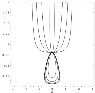
Figure 1 shows a family of contoursH=H1in the(φ, w)
phase-plane, for a cold plasma satisfying the initial con-ditions Eq. (90), i.e., MA2ux0=1, ue0=up0=tanθ, where
θ=60◦. For this initial data, the transverse velocities of the electrons and protons are zero atx=x0in the travelling wave
frame, which is similar to the boundary conditions used by Dubinin et al. (2003). The figure shows the effect of varying the longitudinal flow speedux0fromux0=0.0001 in steps of
0.1 up toux0=2.0. Theux0=0.0001 curve is the nearly
hor-izontal curve passing throughw=3. The parameterux0
in-creases moving clockwise and downwards across the curves on the right hand side of the figure (ux0=0.1(0.1)0.4) until
one encounters the separatrix (ux0≈0.5), which is the
con-tour with the cusps at(φ, w) =(±π/2,0). For the separa-trix,
ux0=
ue0(µ+1)2/µ−tan2θ
2(µ+1)tanθ (124)
(see Appendix C). Settingue0=tanθ=
√
3 2 1 0 1 2 3 0
2 4 6 8 10 12
Φ
w
Fig. 1. H1-level Hamiltonian contours forθ=60◦andMA2ux0=1. In this case ue0=up0=tanθ while ux0 takes the values ux0=0.0001, 0.1(0.1)2.0. (and henceMA varies). The horizontal contour corresponds to aux0value of 0.0001.The separatrix (bold curve) is the contour corresponding toux0=0.5.
the separatrix. The curves inw<3: ux0=0.6(0.1)1.0 for
in-creasing ux0 correspond to a sequence of closed orbits of
decreasing area that converge onto the centre critical point (φ, w)=(0,3) for ux0=1. Note that all the orbits pass
through the same initial point (φ, w)=(0,3) in the phase plane. The contour forux0=1 consists of a single isolated
point(φ0, w0)=(0,3). It is an isolated, centre critical point
ofH. The curves inw>3 correspond toux0=1.1(0.1)2.0,
in whichux0increases monotonically moving outward from
φ=0 in both directions. The tops of the curves are not shown. They consist of a sequence of closed ellipsoidal shaped curves in the regionw≥3, where the topmost points of the curves rise with increasingux0. BecauseMA2ux0=1,
the Alfv´en Mach number of the travelling waves decreases asux0increases. Thus, the largest value ofMAis the curve
ux0=0.0001 for whichMA=100 and the smallest value of
MAisMA=0.7071 obtained whenux0=2.0.
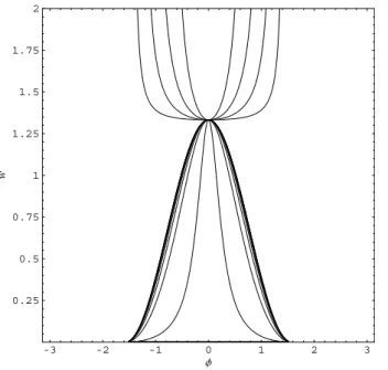
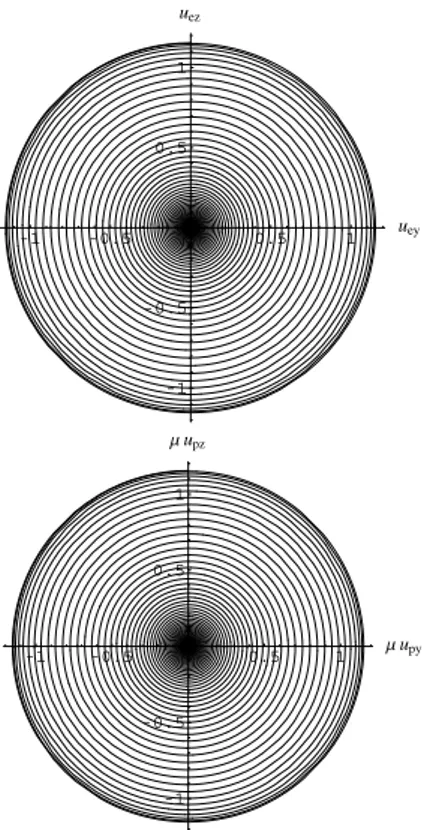
Figure 2 shows phase space trajectoriesH (φ, w)=H1for
θ=30◦, MAe0=0.45, µ=1836 in which ux0 is changed in
steps of 0.02 from ux0=0.0001 to ux0=0.4. The value of
ue0is fixed by the equation:
ue0=
2ux00(µ+1)tanθ
(µ+1)2/µ−tan2θ, (125)
whereux00=0.1. the curveux0=0.1 corresponds to the
sep-aratrix solution andup0is chosen to satisfy the integrability
constraints Eq. (89). Note thatup06=ue0in this example (in
Fig. 1,ue0=up0=tanθ). In the lower plane (w<0.014), the
contours split into two families. The family withux0<0.1
lies outside the separatrix, with the near horizontal curve corresponding toux0=0.0001, andux0increases
monoton-ically moving downward across the curves until the separa-trixux0=0.1 is obtained. Inside the separatrixux0, the closed
loop contours decrease in size with increasingux0until the
centre critical point solution is reached for whichux0=0.2.
3 2 1 0 1 2 3
0.00 0.01 0.02 0.03 0.04 0.05 0.06
Φ
w
Fig. 2. H1-level Hamiltonian contours generated by vary-ing ux0 from 0.02 to 0.4 in steps of 0.02. The value of ue0 was fixed by evaluating the condition for a separatrix ue0=2ux0(µ+1)tanθ/[(µ+1)2/µ−tan2θ]for the particular case ofux0=0.1. In other words the bell-shaped separatrix-like contour (bold curve) corresponds to the caseux0=0.1. The horizontal con-tour corresponds to a value ofux0equal to 0.0001. Other parame-ters are:θ=30◦,MAe=0.45
These contours are bounded inφ (i.e.|φ|<φm<π/2 where
φm is the maximum value of φ). The contours in the
up-per plane in the regionw>0.014 are closed curves withux0
increasing moving upward and outward away from the criti-cal point (ux0=0.4 is the outermost curve inw>0.014). If
one imagines the phase space trajectories (φ (x), w(x)) as wrapped around the surface of a cylinder, where φ is the azimuthal angle, then the solutions are either: (i) bounded in|φ|<φm<π (i.e. the contours inside the separatrix, and in
the upper half planew>0.014) or (ii) the trajectories stretch fromφ= −πtoφ=πand wrap around the cylinder in a con-tinuous, periodic fashion asxchanges.
The above two examples of Hamiltonian trajectories H (φ (x), w(x))=H1 in the (φ, w) phase plane illustrate
phase trajectories in cases where there is a separatrix. How-ever, the existence of a separatrix depends on whether condi-tions Eqs. (C5 and C6) in Appendix C are satisfied.
5.3 The longitudinal structure equation forux
There are further constraints imposed on the travelling wave solutions that are related to the longitudinal structure Eq. (65) describing the dependence ofuxonx, which in present case
reduces to: dux
dx = −
σ (µ+1)ux0cosθ√R(ux)
µux
, (126)
whereR(ux)is given by Eq. (74) but withP=ux0ux,H=H1,
and1W=0, namely:
R(ux)=
2µ(MA2ux0)u2x0
(µ+1)2 (ux−ux0)(u 2