SRef-ID: 1607-7946/npg/2005-12-75 European Geosciences Union
© 2005 Author(s). This work is licensed under a Creative Commons License.
Nonlinear Processes
in Geophysics
Modeling of short scale turbulence in the solar wind
V. Krishan1and S. M. Mahajan2
1Indian Institute of Astrophysics, Bangalore 560 034, India
2Institute for Fusion Studies, The University of Texas at Austin, Austin, Texas 78712, USA
Received: 6 August 2004 – Revised: 17 December 2004 – Accepted: 7 January 2005 – Published: 25 January 2005 Part of Special Issue “Advances in space environment turbulence”
Abstract. The solar wind serves as a laboratory for inves-tigating magnetohydrodynamic turbulence under conditions irreproducible on the terra firma. Here we show that the frame work of Hall magnetohydrodynamics (HMHD), which can support three quadratic invariants and allows nonlinear states to depart fundamentally from the Alfv´enic, is capa-ble of reproducing in the inertial range the three branches of the observed solar wind magnetic fluctuation spectrum – the Kolmogorov branch f−5/3 steepening to f−α1 with
α1≃3−4 on the high frequency side and flattening tof−1on the low frequency side. These fluctuations are found to be as-sociated with the nonlinear Hall-MHD Shear Alfv´en waves. The spectrum of the concomitant whistler type fluctuations is very different from the observed one. Perhaps the relatively stronger damping of the whistler fluctuations may cause their unobservability. The issue of equipartition of energy through the so called Alfv´en ratio acquires a new status through its dependence, now, on the spatial scale.
1 Introduction
Solar wind is a turbulent supersonic outflow of plasma from the solar atmosphere. Fluctuations in the density,the ve-locity and the magnetic fields exist on several spatial and temporal scales. Transient disturbances such as those as-sociated with Solar flare caused blast waves propagate out in the form of various linear and nonlinear plasma waves. Key Observations of the Solar Wind Turbulence have been summarized in Goldstein et al. (1994, 1995). The reduced Spectra of the fluctuations are obtained by averaging over the two directions perpendicular to the solar wind velocity (V). The spectra are a function of the wavenumber along
V. The spectral energy distributions of the velocity and the magnetic field fluctuations in the solar wind are now Correspondence to:V. Krishan
known in a wide frequency range, starting from much be-low the proton cyclotron frequency (0.1–1 Hz) to hundreds of Hz. The inferred power spectrum of magnetic fluctu-ations consists of multiple segments – a Kolmogorov like branch (∝f−5/3) flanked,on the low frequency end by a flat-ter branch (∝f−1) and, on the high frequency end, by a much steeper branch (∝f−α1, α
1≃3–4), (Coleman, 1968; Behan-non, 1978; Denskat et al., 1983; Marsch, 1991; Leamon et al., 1998). Attributing the Kolmogorov branch (∝ f−5/3) to the standard inertial range cascade, initial explanations in-voked dissipation processes (in particular, the collisionless damping of Alfv´en and magnetosonic waves (Gary, 1999; Li et al., 2001), to explain the steeper branch (∝f−α1,α
1≃3–4). However a recent critical study has concluded that damping of the linear Alfv´en waves via the proton cyclotron resonance and of the magnetosonic waves by the Landau resonance, be-ing stronglyk(wave vector) dependent, is quite incapable of producing a power-law spectral distribution of magnetic fluc-tuations; damping mechanisms lead, instead, to a sharp cut-off in the power spectrum. Cranmer and Ballogoeijen (2003) have however, demonstrated a weaker than an exponential dependence of damping on the wave vector by including ki-netic effects. However it is still steeper than that required for explaining the steepened spectrum.
20051). Using dimensional arguments of the Kolmogorov type, we will first derive the fluctuation spectra associated with the velocity and magnetic fields. We then go on to show that in different spectral ranges, different invariants control the energy cascade splitting the inertial range into distinct sections. The steeper and the flatter spectral branches (to-gether with the standard branch), then, are all sub-parts of the extended inertial range. Invoking the hypothesis of selective dissipation, we then construct the entire magnetic spectrum with its three branches and two breaks by stringing together three spectral segments each controlled by one of the three invariants.
We briefly describe the nonlinear HMHD in Sect. 2. In Sect. 3, the respective spectral energy distributions are de-rived. The derived spectra are shown to account for the ob-served solar wind spectra in Sect. 4. The attempts invok-ing dissipation and dispersion are reviewed in Sect. 5. A short discussion and a summary of the conclusions consti-tutes Sect. 6.
2 HMHD, nonlinear solution, invariants
In the HALL-MHD comprising of the two fluid model, the electron fluid equation is given by
mene
∂Ve
∂t +(Ve.∇)Ve
=−∇pe−ene
E+1 cVe×B
.(1) Assuming inertialess electrons (me→0), the electric field is found to be:
E= −1
cVe×B−
1
nee
∇pe. (2)
The Ion fluid equation is:
mini
∂Vi
∂t +(Vi.∇)Vi
= −∇pi+eni
E+1 cVi×B
.(3) Substitution for E from the inertialess electron equation begets:
mini
∂Vi
∂t +(Vi.∇)Vi
= −∇(pi+pe)+ 1
cJ×B (4)
The magnetic induction equation becomes:
∂B
∂t = −c∇ ×E= ∇ ×(Ve×B), (5)
whereB is seen to be frozen to electrons. Substituting for Ve=Vi −J/en, one gets:
∂B
∂t = ∇ ×
Vi− J en
×B. (6)
We see thatBis not frozen to the ions,ne=ni=n.
The Hall term dominates for(n e c)−1J×B≥Vi×B/cor
L≤MAc/ωpiandT≥ω−ci1.
1Mahajan, S. M. and Krishan, V.: Exact Nonlinear Hall-MHD
Waves, MNRAS, under submission, 2005.
That is the Hall term decouples electron and ion motion on ion inertial length scales and ion cyclotron times. Hall effect does not affect mass and momentum transport but it does affect the energy and magnetic field transport.
We present, here, an exact solution for Hall MHD (HMHD) allowing an ambient magnetic field which may be a local average in the case of the solar wind.
In the Alfv´enic units withB0as the ambient field,B0=bes,
ks=k·bes is the projection of the wave vector along the di-rection of the field line, and⊥is perpendicular toeˆs. Time and space variables are, respectively, measured in units of the ion gyroperiod ω−ci1=mic/eB0, and the ion skin depth
λi=c/ωpi, whereωpi=(4π e2n/mi)1/2is the ion plasma fre-quency. In the incompressible limit (plasmaβ→∞) we ob-tain the following dimensionless equations
∂B
∂t = ∇ × [(V − ∇ ×B)×B] (7) ∂(B+ ∇ ×V)
∂t = ∇ ×[V ×(B+ ∇ ×V)]. (8)
To look for wave like solutions’ we split the fields into their ambient and the fluctuating parts (there is no ambient flow),
B=bes +b; V =v (9)
and substitute in Eqs. (7)–(8),
∂b
∂t = ∇ ×[(v− ∇ ×b)×bes +(v− ∇ ×b)×b] (10) ∂
∂t(b+ ∇ ×v)= ∇ ×[v×(∇ ×v+b)+v×bes]. (11)
The nonlinear problem represented by Eqs. (10)–(11) is con-verted to a set of linear problems (the time honored method for solving nonlinear equations) by imposing the following conditions to eliminate the nonlinear terms:
v− ∇ ×b=αb (12)
b+ ∇ ×v=βv, (13)
where αandβ are like the separation constants. With the nonlinearities so taken care of, we are left with the remaining time dependent linear equations
∂b
∂t =α∇ ×[b×bes] (14)
∂
∂t(v)=(1/β)∇ ×[v×bes]. (15)
Apparently we have traded a close nonlinear system (6 equa-tions for six variables) for an overdetermined linear system (Eqs. 12–15) with 12 equations in six variables. Acceptable solutions, therefore, will be possible only under some partic-ular conditions that will remove the over determination. To seek them, we first notice that Eq. (14) and Eq. (15) admit
b=bkexp(ik
¯·x¯+iα(bes·k¯)t ) (16)
v=vkexp
ik ¯·x¯+i
1
β(bes·k¯)t
If the exponential solutions (Eq. 16) and (Eq. 17) are to satisfy the linear equations (12) and (13), we must require
β = 1/α. In addition, substituting Eqs. (16) and (17) into Eqs. (12) and (13) leads to
vk−ik
¯×bk =αbk, (18)
bk+ik ¯×vk=
1
αvk, (19)
which, after simple manipulation, yield
vk−αbk =iαk
¯×vk (20)
vk−αbk =i(k
¯×bk). (21)
Two consequences immediately follow:
bk=αvk (22)
relatingbkandvk, and k
¯×vk = −i 1−α2
α vk= −iλvk. (23)
The first of these establishes the HMHD equivalent of the Alfv´enic condition for MHD and the second, the Fourier transform of a Beltrami equation (∇×G
¯=λG¯) has to be solved to complete the story; the solvability constraint will end up relating α with k giving the “dispersion relation”
α=α(k).
The solutions of Eq. (23) are well-known and we could just quote them. But for completeness, we recapitulate a few steps in the process. Suppressing the indices for a simplified notation, we derive from Eq. (23): 1) dotting withvyields
v·v=v2r−v2i+2ivr·vi=0 implyingvi=0±vr, 2) and dotting with k
¯gives k¯·v=0⇒k¯·vr=0=k¯·vi. The suffixr(i)denotes the real(imaginary) part. Crossing Eq. (23) with k
¯and using k
¯·v=0, we obtain the dispersion relation (remembering that
λis a function ofα)
λ= ±k. (24)
Keeping track of the ± may be notationally complicated. Since the physics is the same, we will investigate the option,
vi=vrandλ=k. For this choice, it is straightforward to show thatbvr,vbi, andbk
¯form a right-handed orthogonal triad of unit vectors.
Let us first choosebvr,bvi, andbk
¯to bebex,bey, andbez, respec-tively. This choice dictates the following expressions for the velocity and the magnetic fields (k
¯=kbez, andA0is a constant amplitude);
b=αv, (25)
v=A0[bex+ibey]exp(ikz+iαk(bez·bes)t ) (26) withαdetermined by
k=λ=1−α
2
α , (27)
α±= −k
2 ±
k2
4 +1 !1/2
. (28)
From Eqs. (26) and (28), we extract the effective frequency of the circularly polarized wave,
ω±= −k −k
2 ±
k2
4 +1 !1/2
(bez·bes), (29)
a result which is valid over a wide range ofkfromk≪1 MHD end to thek≫1 Hall dominated regime. Thekdependence of the separation constant, implying akdependent relationship betweenb andv is one of the defining and distinguishing characteristics of the new broadband fully nonlinear incom-pressible wave. To make contact with the familiar, let us ex-amine the two extreme limits of the general result. Fork≪1,
α→ ±1, ω→ ∓k(bez·bes), (30) reproducing thek independent MHD Alfv´enic relationship for both the co- and the counter propagating waves. In the
k≫1 regime, however,
α+→1/ k, α−→ −k, (31)
with
ω+→ −bez·bes, ω−→(bez·bes)k2. (32) It is easy to recognize, in analogy with the linear theory, that the (+) wave is the shear-cyclotron branch, while the (−) rep-resents the whistler mode. the frequency of the (+) wave approaches some fraction of the ion gyro frequency (normal-izing frequency) – it is only when k
¯andB0are fully aligned
(bez·bes=±1)that the wave reaches the cyclotron frequency asymptotically. In this limit the magnitudes of the veloc-ity and magnetic fields can vastly differ (they still remain aligned). The respective relationships are
v→kb. (33)
for the(+)branch, and
b→kv. (34)
for the (−) branch; the compressional-whistler mode is dom-inated by the magnetic energy, while in the shear-cyclotron mode, the kinetic energy dominates.
The well-known invariants of the HMHD system (Maha-jan and Yoshida 1998),
Total energy:
E=1
2 Z
(v2+b2)d3x= 1
2 X
k
|vk|2+ |bk|2 (35)
Magnetic helicity:
HM = 1 2
Z
A· Bd3x =1
2 X
k
i
k2(k×bk)·b−k (36)
Generalized helicity:
HG= 1 2
Z
(A+V)·(b+∇×v)d3x
= 1
2 X
k
ik×bk k2 +vk
·v−k−ik×v−k
k k
k k
Power
Power
k k
k
k W
W
k
k W
M
M
M k
k
k
k
W W
M M
M
W B > V
(a) (b)
H
E
G H
E
G
H G
H G
E
E
k k
−7/3 −5/3
1/3
−7/3 1
1
−13/3 −11/3
1 1
1
1 −5/3
−1/3
−1
−3
1 2
Fig. 1. (a)Schematic Magnetic(M)and Kinetic(W )spectra (Shear-cyclotron mode) forα=k−1in the Hall region(k≫1),(b)Schematic Magnetic(M)and Kinetic(W )spectra (Whistler mode) forα=kin Hall region(k≫1).
whereAis the vector potential. Notice thatHG−HM is a combination of the kinetic and the cross helicities.
Notice that the relationship betweenvk andbk is nowk dependent. It is expected, therefore, that the current spectral predictions will be substantially different from those of the standard MHD (wherevkandbkhave identical spectra) par-ticularly in the rangek≫1, when the Hall term dominates in Eq. (6). The introduction of the Hall term, which brings in an intrinsic scale removes the MHD spectral degeneracy and generates new scale-specific effects.
3 Spectral energy distributions
The nonlinear solution is an exact solution for waves prop-agating in one direction. For the superposition of the right and the left propagating waves the nonlinearity remains and this is what could give rise to the cascading processes as is surmised in the ideal MHD turbulence. The large wavevec-tor limit of the dispersion relation of the nonlinear waves basically leads to the dispersive effects with the difference that now the relation between the velocity and the magnetic field amplitudes is also wave vector dependent. With these qualifying remarks we proceed to derive the spectral energy distributions using the Kolmogorov hypotheses according to which the spectral cascades proceed at a constant rate gov-erned by the eddy turn over time(kvk)−1. ForεE denoting the constant cascading rate of the total energy E, Eq. (35) along with Eq. (22) yields the dimensional equality
(kvk)[1+(α)2]
v2k
2 =εE. (38)
The omnidirectional spectral distribution function WE(k) (kinetic energy per gram per unit wave vectorv2k/ k), then, takes the form
WE(k)= 2εE
2
3 [1+(α)2]−23k−53. (39)
Consequently, Eq. (22) yields:
ME(k)=(α)2WE(k). (40)
whereME(k)=b2k/ kis the similarly defined omnidirectional spectral distribution function of the magnetic energy density. The cascading of the magnetic helicityHM (εH being the
cascading rate for helicity) produces a different dimensional equality
(kvk) 0.5
b2k
k !
=εH (41)
resulting in the following different kinetic and magnetic spectral energy distributions:
WH(k)=(2εH)
2
3 (α)
−4
3 k−1, (42)
MH(k)=(α)2WH(k). (43)
Finally, the cascading of the generalized helicity with a con-stant rateεGgives
(kvk) h
0.5g(k)vk2 i
=εG, (44)
g(k)=(α+k)2k−1
leading to the spectral energy distributions:
WG(k)= 2εG
2
3 [g(k)]−23k− 5
3, (45)
and
4 Modeling solar wind spectra
The observed frequency spectra of the solar wind are trans-formed into the wave vector spectra Doppler shifted by the Super Alfv´enic Solar wind flow. Although the anisotropy of the MHD turbulence is now being highly emphasized (Matthaeus et al., 1996), we model the observed reduced om-nidirectional spectra with the findings of the isotropic cas-cade considered in Sect. 3. The incompressible nonlinear so-lution applies essentially to a plasma withβ→∞case. The plasmaβ for the solar wind varies from less than to much larger than unity. Here we neglect compressibility effects and highlight the crucial contributions of the Hall effect through the shear Alfv´en modes as the steepening of the solar wind spectra appears near the ion inertial scale, a characteristic of the Hall effect. It is not clear from the observations if the density fluctuations also has a characteric scale comparable to the ion inertial scale. It is well known that weak compress-ibility (v≪sound speed) makes a very small change in the Kolmogorov (−5/3) spectrum. The kinetic energy spectra is also not well known in this region. In the absence of such information for simplicity we resort to the incompressibility assumption and show that the three spectral distributions de-rived in Sect. 3 may model the three branch spectrum (k−1,
k−5/3,k−α1α
1≃3−4) of the magnetic fluctuations in the so-lar wind.
If the turbulence is dominated by velocity field fluctuations (v2
k≫b 2
k) (which happens, according to Eq. (22), for (α≪1), or (k≫1) for α≃(k−1), the spectral expressions under the joint dominance of the Hall term and the velocity fluctuations (k≫1) simplify to (Fig. 1)
WE1(k)=(2εE)
2/3k−5/3, M
E1(k)=(2εE)
2/3k−11/3 (46)
WH1(k)=(2εH)
2/3k1/3, M
H1(k)=(2εH)
2/3k−5/3 (47)
WG1(k)=(2εG)
2/3k−7/3, M
G1(k)=(2εG)
2/3k−13/3. (48) In the case whereinα=1 fork≪1, one obtains the standard Alfv´enic state with vk∝bk, and the corresponding spectra (Fig. 2) are (suffix 1 is used for the Hall Dominant and 2 for the standard MHD limit):
M(k)=W (k) (49)
WE2(k)=(2εE)
2/3k−5/3 (50)
WH2(k)=(2εH)
2/3k−1
(51)
WG2(k)=(2εG)
2/3k−1
(52) For the second root ofα≃k,k≫1, representing theβ→∞
limit of the whistler type fluctuations, we find the following spectra:
WEw(k)=(2εE)
2/3k−3, M
Ew(k)=(2εE)
2/3k−1 (53)
WHw(k)=(2εH)
2/3k−7/3, M
Hw(k)=(2εH)
2/3k−1/3 (54)
WGw(k)=(2εG)
2/3k−7/3, M
Gw(k)=(2εG)
2/3k−1/3. (55)
k
k k
Power
W k k
W k
W
E H
E
1
−5/3 −5/3
2
−1
3 4
2
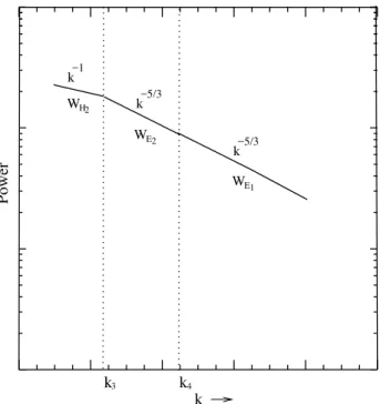
Fig. 2. Schematic Magnetic(M)and Kinetic(W ≡ M)spectra (shear-Alfv´en mode) forα≃1 in the Alfv´en region(k≪1).
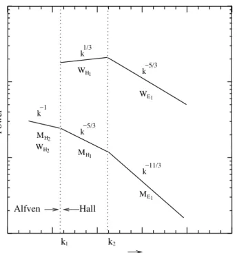
The observed solar wind magnetic spectrum will be gen-erated if we were to string together the three branches
ME1(k)(∝k
−11/3), M
H1(k)(∝k
−5/3), and M
H2(k)(∝k
−1). The rationale as well as the modality for stringing differ-ent branches originates in the hypothesis of selective dissipa-tion. It was, first, invoked in the studies of two-dimensional hydrodynamic turbulence (Fjortoft, 1953; Hasegawa, 1985). In 2-D hydrodynamic turbulence, for instance, the enstro-phy invariant, because of its stronger k dependence (and hence larger dissipation) compared to the energy invariant, dictates the largekspectral behavior. Therefore, the entire inertial range spectrum has two segments – the energy dom-inated low k(∝k−5/3), and the enstrophy dominated high
k(∝k−3). The procedure amounts to placing the spectrum with the highest negative exponent(∝k−13/3)at the highest
k-end,then the spectrum with the next lower negative expo-nent(∝k−11/3)and finally the one with the lowest negative exponent ofkat the lowestk-end (e.g. Fig. 1a).
Notice that the observed solar wind magnetic spectra con-sisting of the branchesk−α1 (α
Alfven Hall
k k
Power
W
M
M W W
k
k
M k
k
k H
H
E E H
H 2
1
1 1 1
1/3
−5/3
2
−1
−5/3
−11/3
1 2
Fig. 3.Modeled Magnetic(M1)spectra along with the correspond-ing Kinetic(W1)spectra.
5 Hall time scale
From the magnetic induction equation
∂
∂tB= −c∇ ×E = ∇ ×(Vi−J)×B (56)
one can identify a characteristic Hall time scale
τH = [k(Vi +VH)]−1 (57) where VH=−J is the hall velocity. Thus
τH=[k(vk + kbk)]−1=[k(vk+kαvk)]−1=(2kvk)−1 for
bk=αvkandα=k−1.
Thus the Hall time scale is half the hydrodynamic time scale for Hall shear Alfv´enic fluctuations. This is a further confirmation that the combination of the hydrodynamic time scale along with the association of fluctuations with the shear Alfv´en waves is the right choice for reproducing the observed spectra.
6 Dissipative and dispersive attempts
The diffusion equation for the omnidirectional spectral den-sityW can be written as (Li et al., 2001):
∂W ∂τ =
∂ ∂k
" k2D∂(k
−2W )
∂k #
+γ W+S (58) For a power law form:
W (k)=W0k−s (59)
In the steady state, in the absence of the sourceSand dissipa-tion or growthγ, the diffusion coefficientD∝k1+s. Fors=3,
0.0 0.2
Hall Alfven
0.4 0.6 0.8 1.0
k k
0.01 0.10 1.00 10.00
Power
W k
W
W M
M M
k
k
k E
H
E H
E E
1
−5/3
2
2 2
1 2
−1
−5/3
−11/3
3 4
Fig. 4.Modeled Magnetic(M2)spectra along with the correspond-ing Kinetic(W2)spectra.
D∝k4. This is achieved by definingD=k2/τand identifying
τ with the inverse of the frequency of the whistler mode so thatτ≈ω−1∝(k+k2)−1, leading to the so called dispersion range of the spectrum for s=3 (Stawicki et al., 2001). We wish to comment that identifying the cascade timeτwith the wave period is not correct since the cascade is a nonlinear process and its time scale should be a function of the fluctu-ation amplitude.
The attempts to account for the steepened spectrum by in-voking dissipation fail (Gary, 1999; Li et al., 2001) as can be seen from the following considerations. The diffusion equa-tion for the omnidirecequa-tional spectral densityWin the steady state with dissipation and no source can be written as:
∂ ∂k[k
2D∂(k−2W )
∂k ] +γ W =0. (60)
With D=k2/τ≈k2(kv
k)=k3[kW (k)]0.5∝k(7−s)/2 we find
γ∝k(3−s)/2. Thus for the steepened spectrum with s=3,
γ∝k0and fors=4,γ∝k−0.5. But the damping of the Alfv´en waves by the ion- cyclotron resonance absorption has an ex-ponential dependence onk and the damping of the magne-tosonic waves by Landau resonance has a power law depen-dence much stronger thank−0.5. Thus the dissipation pro-cesses are inadequate to account for the steepened part of the solar wind spectrum.
7 Discussion and conclusions
and dispersive ranges invoked in some earlier studies. The observed turbulent fluctuations are shown to be associated with Hall shear Alfv´en waves cascading with the hydrody-namic timescale also the Hall timescale. The scale depen-dent relationship between the velocity and the magnetic fluc-tuations redefines the concepts of the equipartition of energy and the Alfv´en ratio. These along with the kinetic energy spectrum offer further possibilities of validation of this exact nonlinear incompressible HMHD model of turbulence. The compressibility effects which will in general not permit an exact solution have to be necessarily studied in a linearized version of HMHD.
Acknowledgements. The authors gratefully acknowledge the support from the Abdus Salam International Center for Theoretical Physics, Italy where a part of the work was done. The authors thank B. Varghese for his help in the preparation of this manuscript. The authors thank the referees for their critical comments and helpful suggestions
Edited by: T. Passot Reviewed by: two referees
References
Behannon, K. W.: Heliocentric distance dependence of the in-terplanetary magnetic field, Reviews of Geophysics and Space Physics, 16, 125–145, 1978.
Biermann, L.: Komentenschweife und solare korpuskularstrahlung, Z. Astrophys., 29, 274–286, 1951.
Chapman, S.: On outline of a theory of magnetic storms, Proc. Roy. Soc. A, 95, 61–83, 1919.
Coleman, P.J. Jr.,: Turbulence, viscosity, and dissipation in the Solar wind plasma, Astrophys. J., 153, 371–388, 1968.
Cranmer, S. R. and von Ballagooijen, A. A.: Alfv´enic turbulence in theextended solar corona: kinetic effects and proton heating, Astrophys. J., 594, 573–591, 2003.
Denskat, K. U., Beinroth, H. J., and Neubauer, F. M.: Inter-planetary magnetic field power spectra with frequencies from 2.4×10⁻⁵Hz to 470 Hz from HELIOS-observations during solar minimum conditions, J. Geophys., 54, 60, 1983.
Gary, S. P.: Collisionless dissipation wavenumber: Linear theory, J. Geophys. Res., 104, 6759–6762, 1999.
Ghosh, S., Siregar, E., Roberts, D. A., and Goldstein, M. L.: Simulation of high-frequency solar wind power spectra using Hall magnetohydrodynamics, J. Geophys. Res., 101, 2493–2504, 1996.
Goldstein, M. L., Roberts, D. A., and Fitch, C. A.: Properties of the fluctuating helicity in the inertial and dissipation ranges of solar wind turbulence, J. Geophys. Res., 99, 11 519–11 538, 1994. Goldstein, M. L., Roberts, D. A., and Matthaeus, W. H.:
Magneto-hydrodynamic turbulence in the solar wind, Annual Rev. Astron. Astrophys., 33, 283–325, 1995.
Hasegawa, A.: Self-organization processes in continuous media, Adv. Phys., 34, 1–42, 1985.
Krishan, V. and Mahajan, S. M.: Hall-MHD turbulence in solar atmosphere, Solar Physics, 220, 29–41, 2004.
Leamon, R. J., Smith, C. W., Ness, N. F., Matthaeus, W. H., and Wong, H. K.: Observational constraints on the dynamics of the interplanetary magnetic field dissipation range, J. Geophys. Res., 103, 4775–4787, 1998.
Li, H., Gary, P., and Stawicki, O.: On the dissipation of magnetic fluctuations in the Solar wind, Geophys. Res. Lett., 28, 1347– 1350, 2001.
Mahajan, S.M. and Yoshida, Z.: Double Curl Beltrami Flow: dia-magnetic structures, Phys. Rev. Lett., 81, 4863–4866, 1998. Marsch, E.: MHD turbulence in the solar wind, in Physics of the
Inner Heliosphere II, Particles, Waves and Turbulence, edited by Schwenn, R. and Marsch, E., Springer-Verlag, New York, 1991. Matthaeus, W. H., Ghosh, S., Oughton, S., and Roberts, D. A.: Anisotropic three-dimensionsl MHD turbulence, J. Geophys. Res., 101, 7619–7629, 1996.
Parker, E. N.: Dynamics of the interplanetary gas and magnetic fields, Astrophys. J., 128, 664–676, 1958.