Application of optical tomography in the study of discolouration in drinking water distribution systems

(1)

DWESD

4, 39–59, 2011

Application of optical tomography in the

study of discolouration

P. van Thienen et al.

Title Page

Abstract Introduction

Conclusions References

Tables Figures

◭ ◮

Back Close

Full Screen / Esc

Printer-friendly Version Interactive Discussion

Discussion

P

a

per

|

Dis

cussion

P

a

per

|

Discussion

P

a

per

|

Discussio

n

P

a

per

|

Drink. Water Eng. Sci. Discuss., 4, 39–59, 2011 www.drink-water-eng-sci-discuss.net/4/39/2011/ doi:10.5194/dwesd-4-39-2011

Drinking Water

Engineering and Science

Discussions

O

p

en

Acc

e

s

This discussion paper is/has been under review for the journal Drinking Water Enginee-ring and Science (DWES). Please refer to the corresponding final paper in DWES if available.

Application of optical tomography in the

study of discolouration in drinking water

distribution systems

P. van Thienen, R. Floris, and S. Meijering

KWR Watercycle Research Institute, P.O. Box 1072, 3430 BB Nieuwegein, The Netherlands

Received: 10 May 2011 – Accepted: 21 May 2011 – Published: 27 June 2011

Correspondence to: P. van Thienen ([email protected])

Published by Copernicus Publications on behalf of the Delft University of Technology.

(2)

DWESD

4, 39–59, 2011

Title Page

Tables Figures

◭ ◮

Back Close

Full Screen / Esc

Discussion

P

a

per

|

Dis

cussion

P

a

per

|

Discussion

P

a

per

|

Discussio

n

P

a

per

|

Abstract

Theories describing the turbulent deposition of particles from aerosols have recently been applied to drinking water distribution. In order to allow the study of these pro-cesses in a quantitative way and internally observe a cloud of suspended particles in a pipe, we have developed an optical tomography technique and measuring device

us-5

ing low cost electronic components specifically for this application. The mathematical methodology and the electronic device are described in this paper, and tests of both the mathematical approach and the actual device are presented. We conclude that the described methodology may provide a valuable tool for the study of processes related to drinking water discolouration in the lab.

10

1 Introduction

Water discolouration continues to be one of the prime reasons for customer complaints relating to water quality to be received by water companies (Husband and Boxall, 2011). The resuspension of particles present in the drinking water distribution sys-tem by a hydraulic disturbance is usually invoked to explain its occurrence (Vreeburg

15

and Boxall, 2007). A chain of events or processes can be identified in the genera-tion of a discolouragenera-tion event, i.e. origin, evolugenera-tion, deposigenera-tion, cohesion/adhesion and resuspension of particles.

The suggestion that currently applied models do not encompass the complete range of physical processes responsible for the occurrence of discolouration (Blokker et al.,

20

2010) has led van Thienen and Vreeburg (2010) and van Thienen et al. (2011b) to the-oretically investigate the possibility of processes other than gravitational settling aff ect-ing particle deposition. Their findect-ings predict the occurrence of the turbulent process of turbophoresis under specific conditions which may be expected in transport mains. In order to experimentally verify these predictions, a method of internally observing a

25

(3)

DWESD

4, 39–59, 2011

Title Page

Tables Figures

◭ ◮

Back Close

Full Screen / Esc

Discussion

P

a

per

|

Dis

cussion

P

a

per

|

Discussion

P

a

per

|

Discussio

n

P

a

per

|

required methodology, of which a preview has been presented by van Thienen et al. (2011a), is developed using the principles of optical tomography. The method allows its user to study particle transport, deposition and resuspension behaviour in a transpar-ent pipe both qualitatively (in terms of different structures in the particle concentration field relating to di_fferent mechanisms) and quantitatively (in terms of radial transport

5

velocities). The technique uses a sophisticated inversion scheme to include and deal with the effects of measurement uncertainties and noise.

Tomography is a well established technology in the field of medicine (see e.g. Bibb and Winder, 2010), allowing doctors a non-destructive view inside a patient. It is also used e.g. in geophysics to view inside the Earth using seismic waves (e.g. Bijwaard

10

and Spakman, 1999), and has been applied to industrial gravity chutes (Zheng et al., 2006). However, its application in drinking water research is new.

2 Methodology

2.1 Principle

In the present application, we use visible light to internally observe a moving volume of

15

water containing suspended particles. Light is shone through a perspex pipe perpen-dicular to the pipe direction from several points and at several angles of incidence. At the same time, the transfer of this light through the perspex pipe and the particle bear-ing water it is filled with is measured. Scatterbear-ing and absorption reduce the intensity of the light falling on the sensors. By mathematically combining these measurements, a

20

clear image of the cross-sectional particle concentration field can be obtained.

2.2 Measuring device set-up

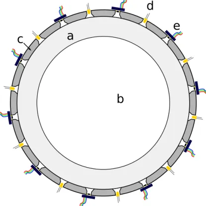
A PVC ring containing ten evenly spaced LEDs with ten evenly spaced sensors in-between is fixed around the transparent tube (see Fig. 1). The LEDs are high-power

(4)

DWESD

4, 39–59, 2011

Title Page

Tables Figures

◭ ◮

Back Close

Full Screen / Esc

Discussion

P

a

per

|

Dis

cussion

P

a

per

|

Discussion

P

a

per

|

Discussio

n

P

a

per

|

white LEDs; the sensors are Phidget light sensors (Phidgets, 2010). An Arduino Mega micro-controller (Arduino, 2010) with custom software is used to control the LEDs (us-ing switch(us-ing electronics) and also contains the AD-converters which are used to dig-itally read the light sensors (10 bit resolution). The Arduino board is connected to a computer using a USB cable. At regular intervals (typically a few seconds), the LEDs

5

are briefly switched on successively. While a single LED is illuminated, all light sensors are read. This entire measurement cycle takes only a fraction of a second. When all sensor readings have been collected, they are sent to the computer for processing. We note that the measuring device was constructed exclusively from low cost components.

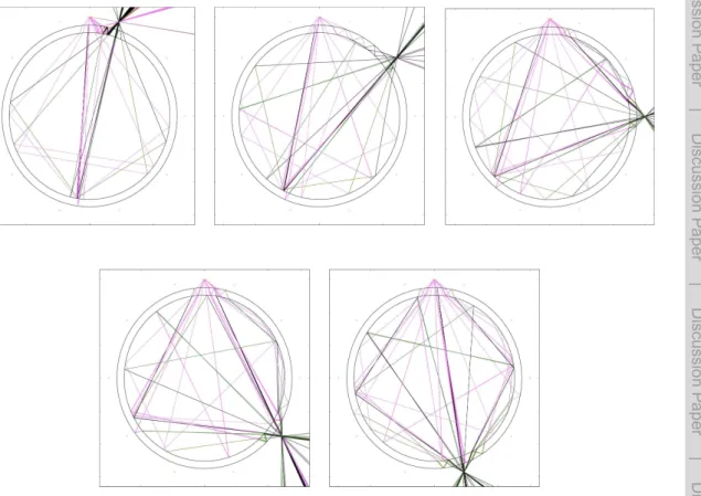
2.3 Refraction and reflection 10

Because of significantly different optical densities, light is refracted and reflected both at the air-perspex interfaces and at the perspex-water interfaces. The Fresnel equa-tions (see e.g. Brass, 2010) allow the calculation of the relative amounts of light which are reflected and refracted. Snell’s law subsequently provides the angle of refraction. Based on these expressions, light beams can be traced from their emission from the

15

LED to their absorption by a sensor. Figure 2 shows a set of light beams shone into the perspex pipe from the center of the light emitting surface of a single LED at different angles of incidence. Light can be seen to reach all sensors through combinations of reflections and/or refractions with different intensities (indicated by colour). In the case where LED and light sensor are adjacent (Fig. 2a), most light falling on the sensor

20

comes from a reflection on the outside of the perspex pipe and as a result does not contain any information on the light absorption by material inside the pipe. The other cases (Fig. 2b–e), however, show that most light reaching the sensors follows the most direct route through the pipe, i.e. by respective refraction at the air-perspex, perspex-water, opposite water-perspex, and opposite perspex-air transitions, which is generally

25

(5)

DWESD

4, 39–59, 2011

Title Page

Tables Figures

◭ ◮

Back Close

Full Screen / Esc

Discussion

P

a

per

|

Dis

cussion

P

a

per

|

Discussion

P

a

per

|

Discussio

n

P

a

per

|

2.4 Mathematical description

2.4.1 Physical assumptions

In the following, a number of assumptions will be made. These are:

– The fraction of light which is scattered by suspended particles increases in some way with the particle concentration. As a result, the relative amount of light which

5

passes through the suspension decreases with increasing particle concentration.

– A simple optical model is used in which particles only cast shadows and their concentration is sufficiently low for particles not to be in each other’s shadows. No scattering or reflection of light offparticles is taken into account.

2.4.2 Model set-up 10

The cross-sectional domain is discretized into a number of triangles. On the corners of each of these triangles, an (initially unknown) light absorption coefficient is defined. For each light beam (path from LED to light sensor), an equation can be written which describes the decrease in intensity of the light beam as a function of the (unknown) light absorption coefficients. The relative light intensity decrease can be written as the

15

ratio of the intensity decrease to the reference intensity: ₍_I

E − IR)

IE

= Σn_j₌1

Z

path

c(l) dl (1)

In this expression, IE is the unperturbed or reference light intensity at the receiver

and IR is the measured light intensity at the receiver in the perturbed experimental

situation. A summation is made over allnelements in the discretization, and the

un-20

known absorption or “shadow” coe_fficients care integrated over the path of the light beam inside each of the elements it passes through. Combining all measurements

(6)

DWESD

4, 39–59, 2011

Title Page

Tables Figures

◭ ◮

Back Close

Full Screen / Esc

Discussion

P

a

per

|

Dis

cussion

P

a

per

|

Discussion

P

a

per

|

Discussio

n

P

a

per

|

((IE−IR)/IE)i in a vectorr, all unknown absorption coefficientscin a vectors, and all

integration coefficients in a matrixA, we get a system of equations:

As = r (2)

Solving this system of equations is an inverse problem.

2.5 Light beam paths 5

As indicated in Sect. 2.3, light reaches the sensors through a complex set of paths which contribute in varying amounts to the total signal. However, in most cases, 98 % or more of the light which reaches a sensor arrives through a direct path without reflec-tions. Therefore, a simple approximation of this set of paths, a straight line connecting a LED to a beam, can be applied instead. In the following, we apply both this simple

10

approximation (single beam model) and a full set of light paths (multiple beam model).

2.5.1 Inversion procedure

When the number of beams is equal to the number of unknown coefficients, in prin-ciple we have a determined system of equations, which can possibly be solved. This would result in knowing the values of the light absorption coe_fficients in all nodes of the

15

discretization, which are a proxy for the local particle concentration. However, mea-surement and discretization errors dominate the result if this procedure is applied. In addition to this, refraction and incidental low beam intensities reduce the number of beams which can actually be used, resulting in a underdetermined problem. A more refined inversion procedure is required to get meaningful results. Suitable methods

20

(7)

DWESD

4, 39–59, 2011

Title Page

Tables Figures

◭ ◮

Back Close

Full Screen / Esc

Discussion

P

a

per

|

Dis

cussion

P

a

per

|

Discussion

P

a

per

|

Discussio

n

P

a

per

|

Applying these methods (Tarantola, 2005; Muntendam-Bos et al., 2008), the system (Eq. 2) is rewritten as:

s = C_mAT

A C_mAT ₊ C_d−1 r (3)

In this expression,Cm is the covariance matrix of the prior model matrix. It is

pro-duced by computing the covariance matrix for a large number of plausible models which

5

span the parameter space of expected results, and contains all prior knowledge, un-certainties and variations of the model. Cd is the prior data covariance matrix, which

has the variances σ2 of the measurements on the main diagonal and zeros o_ff the main diagonal. The total variances consist of the actual measurement variancesσ_{mi j}2 which are obtained for each LED-sensor combinationij from multiple samples which

10

are taken and a system varianceσs2which is assumed to be the same for all

measure-ments and includes all errors which are not included inσm2. A representative value of

σsis chosen. The variances are summed following Bienaym ´e’s formula:

σ_{i j}2 = σ_{mi j}2 + σs2 (4)

2.5.2 Resolution and covariance 15

In order to understand what quality of results can be expected from the inversion pro-cedure, we compute the resolution matrix and compare prior and posterior covariance matrices. The resolution matrix is defined as (Tarantola, 2005; Muntendam-Bos et al., 2008):

R = CmAT

A CmAT + Cd

−1

A (5)

20

For a perfectly resolved system, the resolution matrix is equal to the identity matrix. The posterior covariance matrix can be computed from the resolution matrix (Taran-tola, 2005; Muntendam-Bos et al., 2008):

C ₌ (I − R)Cm (6)

(8)

DWESD

4, 39–59, 2011

Title Page

Tables Figures

◭ ◮

Back Close

Full Screen / Esc

Discussion

P

a

per

|

Dis

cussion

P

a

per

|

Discussion

P

a

per

|

Discussio

n

P

a

per

|

This expression shows that a well-resolved posterior model with low variances is obtained for a model which has a resolution matrix close to the identity matrix. Also, it is clear from Eq. (6) that uncertainties in the prior model directly propagate into the posterior model. The magnitude of this propagation depends on the resolution. For a resolved system, posterior variances should be smaller than prior variances.

5

We shall use matricesRandCto evaluate the mathematical quality of the results of the inversion procedure.

3 Tests

3.1 Mathematical approach

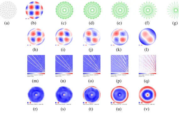
A series of simulations has been performed in order to assess the capabilities and limits

10

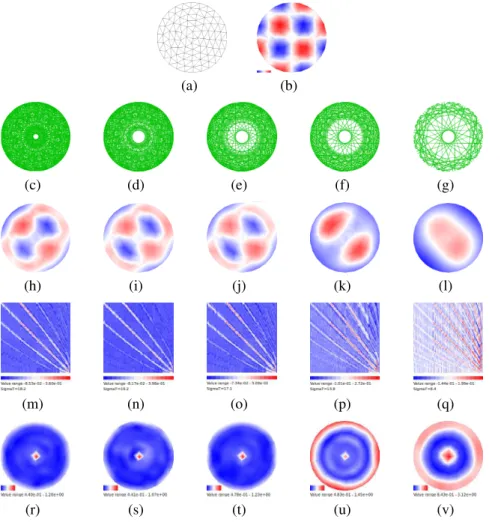
of the mathematical model in the context of the measurement device setup. Figure 3 summarizes the results of these tests for a single beam model (see Sect. 2.5). Fig-ure 4 does the same for a multiple beam model as described in Sect. 2.3. A synthetic light absorption coefficient field was generated exhibiting a checkerboard pattern (see Figs. 3b and 4b). Corresponding synthetic measurements were computed for all beams

15

based on this pattern (10 samples per beam), adding white noise to the measurements with a maximum amplitude of 10 %. These synthetic measurements were fed into the inversion procedure, assuming all uncertainty to originate from the measurement er-ror (Eq. 4,σs=0). For different beam sets displayed in Fig. 3c–g, this results in the

corresponding tomograms of Fig. 3h–l for the single beam model and Fig. 4h–l for the

20

multiple beam model. Traditionally, checkerboard tests have often been used to illus-trate the quality (or lack thereof) of an inversion procedure (e.g. Morgan et al., 2002). In the tomograms of Figs. 3h–l and 4h–l, a decreasing correspondence with the original synthetic input field (Figs. 3b and 4b) can be observed for decreasing beam coverage. However, in frames h, i and j, the reconstructed image is still acceptably close. An

25

(9)

DWESD

4, 39–59, 2011

Title Page

Tables Figures

◭ ◮

Back Close

Full Screen / Esc

Discussion

P

a

per

|

Dis

cussion

P

a

per

|

Discussion

P

a

per

|

Discussio

n

P

a

per

|

means of the resolution and posterior covariance matrices, as defined in Sect. 2.5.2. As has been indicated above, a resolution matrix is close to the identity matrix for a well resolved model. The sum of the main diagonal of this model indicates how many degrees of freedom are resolved. Figures 3m–q and 4m–q show the resolution matrix for our five different beam coverage scenarios for the single beam model and the

multi-5

ple beam model, respectively. It is clear that in no case is the resolution matrix close to the identity matrix. This means that additional information is taken from the prior model covariance matrix in the inversion procedure. The resulting (posterior) uncertainty in the individual degrees of freedom is plotted in Fig. 3r–v. These images show that the central degree of freedom is not well resolved in all cases compared to the

surround-10

ing area. In addition to this, the degrees of freedom close to the outer wall become increasingly badly resolved as the beam coverage decreases, since it is in this region where the coverage is removed.

Table 1 shows how the maximum value of the prior model covariance matrix com-pares to the maximum value of the posterior model covariance matrix, both for the

15

single beam and the multiple beam optical models. It is clear that in each case, a sig-nificant reduction of the variance is obtained, which means that we have gained infor-mation relative to the prior model. As the available number of observations is reduced by ignoring more measurements – moving from (c) to (g) – the variance reduction does decrease, however. The numbers shown in Table 1 do not show a monotonously

de-20

creasing series for the multiple beam model. This is due to the fact that all numbers are based on simulations with a significant amount of random noise in the input. As a result, all numbers presented are valid for a single simulation but will be somewhat different when the simulation is repeated. However, the presented set of results does illustrate a clear trend.

25

3.2 Inversion results

Now that the theoretical resolvability and resolution have been ascertained, lab tests are required, in which an object representative of a particle cloud is placed inside

(10)

DWESD

4, 39–59, 2011

Title Page

Tables Figures

◭ ◮

Back Close

Full Screen / Esc

Discussion

P

a

per

|

Dis

cussion

P

a

per

|

Discussion

P

a

per

|

Discussio

n

P

a

per

|

the device and located using the device. For this purpose, a curtain was made from wire mesh, which is expected to have optical properties similar to that of a cloud of dark, non-reflecting particles suspended in water and can be easily positioned inside the device (see Fig. 5a and c). This curtain was placed inside the device in different configurations and orientations (Fig. 5b and d). The resulting images are shown in

5

Fig. 5e–g for the single beam model and in Fig. 5h–j for the multiple beam model, for curtain configurations/orientations indicated by a dashed line (note that the actual area occupied by the curtain is wider than the dashed line). The following can be said for all three cases e–g as well as for cases h–j:

– The curtain is well resolved in the tomograms.

10

– The image of the curtain is somewhat wider than the actual curtain.

– The ends of the curtain are not so accurately resolved.

The width can be partially explained from the limited resolution of the tomogram (12 el-ements in its diameter). The ends of the curved curtain in Fig. 5f–g and h–j may be related to the fact that we are imaging an object consisting of lamellae of wire mesh,

15

the visibility of which strongly depends on their orientation relative to the different light beams which are used in its reconstruction in the tomogram. The fact that the linear curtain in Fig. 5e does not appear to touch the walls is a resolution issue. As can be seen in Figs. 3t and 4t, the posterior model variance at the pipe wall is rather large, meaning that this region is not well resolved. This is due to the lack of usable light

20

beams shining more or less parallel to the wall in this region (Fig. 3e). In the case of the multiple beam model, Fig. 3e does show significant beam coverage close to the wall. However, the amount of light carried by these beams is so small that they contribute little to the final tomogram.

In addition to these dry tests, wet tests have been performed with the tomography

de-25

(11)

DWESD

4, 39–59, 2011

Title Page

Tables Figures

◭ ◮

Back Close

Full Screen / Esc

Discussion

P

a

per

|

Dis

cussion

P

a

per

|

Discussion

P

a

per

|

Discussio

n

P

a

per

|

beam field of the measurement device, resulting the tomograms were consistently in agreement with the corresponding actual situation.

4 Discussion

4.1 Functioning

Both the mathematical consideration of the resolution of the inversion results and the

5

dry tests which have been performed show that the device functions as intended. Also, it is capable of resolving particle concentration variations in the inside of a moving body of water which can not be determined by direct observation from the outside. The more complex and computation time consumingmultiple beam modeldoes not appear to result in significantly better images than thesingle beam model, but it does have a

10

better formal resolution close to the wall when ray coverage is reduced.

4.2 Practical considerations

During the test phase of the device, several practical issues were come across and resolved. These include the following:

– Because the variations in light intensity which are the basis of the inversion

pro-15

cedure are relatively small, proper shielding of the device and the section of trans-parent pipe on which it is mounted is essential. In case the shielding is incom-plete, recalibration is required whenever the lighting conditions in the lab change, resettingIEin expression Eq. (1).

– The optical properties of the particles are important in the sense that highly

re-20

flective and/or scattering particles reduce the quality of the inversion results, since reflection and scattering off the particles are not included in the simple optical model which is applied.

(12)

DWESD

4, 39–59, 2011

Title Page

Tables Figures

◭ ◮

Back Close

Full Screen / Esc

Discussion

P

a

per

|

Dis

cussion

P

a

per

|

Discussion

P

a

per

|

Discussio

n

P

a

per

|

4.3 Particle concentrations

In the above, tomograms are obtained which show the distribution of a “light absorption coefficient” throughout a cross-section. This is very useful when one wants to study concentration di_fferences, but the actual concentration values are not obtained. In order to convert absorption coefficients to concentrations, a calibration curve needs

5

to be constructed from experiments with known particle concentrations. It is expected that di_fferent curves are obtained for di_fferent materials with di_fferent optical surface properties.

4.4 Applications

The intended operating environment for the method which has been described in this

10

paper is in the lab. Under normal conditions, the particle concentration in drinking water is much too low to be detectable with the present optical set-up, except when hydraulic disturbances cause discolouration. In the lab, it is possible and often desirable to work with particle concentrations which are much higher than in drinking water distribution systems to facilitate observation and reduce time scales of e.g. accumulation. The first

15

investigation in which this technique has been applied is the experimental verification of a theoretical mechanism map for turbulent particle deposition in drinking water dis-tribution systems (Floris et al., 2011). This presents results describing the conditions of initiation of particle deposition by turbophoresis, building on theoretical predictions by van Thienen et al. (2011b). A number of additional research areas in drinking water

20

(13)

DWESD

4, 39–59, 2011

Title Page

Tables Figures

◭ ◮

Back Close

Full Screen / Esc

Discussion

P

a

per

|

Dis

cussion

P

a

per

|

Discussion

P

a

per

|

Discussio

n

P

a

per

|

4.5 Limitations and possible improvements

Some limitations of the current setup are:

– Since we are considering a moving body of water, we may expect the plug of wa-ter to advance by some distance in the course of the measurement cycle. The resulting image is therefore only meaningful if variations in the particle

concentra-5

tion field do not occur on this time and length scale. At typical flow velocities of 0.01 to 1 m s−1 _{and measurement cycle times (depending primarily on the}

num-ber of samples taken) of 300 to 1500 ms, the length of the imaged plug is 3 mm to 1.5 m.

– The resolution of the tomograms is limited by the number of LEDs and sensors

10

which have been installed.

Several improvement can be made to the device and procedure. We list the most obvious and effective:

– One of the main issues with the current setup is the reduced ray coverage close to the pipe wall due to the effects of refraction. By proper shaping of the outside

15

of the transparent pipe or by choosing a different material with a lower refractive index, this e_ffect can be reduced. For the latter option, however, the choice of alternative materials is not obvious, since the refractive index of perspex is already relatively low.

– Because of the time required to take all measurements, which may add up to

20

hundreds of milliseconds, the image obtained is to some degree an average of the situation over this time period. Using faster electronics would allow a reduction of the measurement time and thus a representation which is closer to a “real” snapshot.

(14)

DWESD

4, 39–59, 2011

Title Page

Tables Figures

◭ ◮

Back Close

Full Screen / Esc

Discussion

P

a

per

|

Dis

cussion

P

a

per

|

Discussion

P

a

per

|

Discussio

n

P

a

per

|

– A more sophisticated optical model including light scattering (and possibly reflec-tion) by particles should increase the accuracy of the tomograms and allow the use of a wider range of particle materials.

– Finally, the resolution of the obtained images can be increased by increasing the number of light paths through the number of LEDs and/or sensors.

5

5 Conclusions

The presented methodology provides a useful and promising technique for the study of several areas in drinking water discolouration research. The first application of the device and methodology is presented in Floris et al. (2011).

Acknowledgements. We thank Karin van Thienen-Visser for help with the inversion procedure,

10

Melanie Tankerville for reviewing the English of this paper, and Mirjam Blokker for helpful com-ments on the manuscript.

References

Arduino: http://www.arduino.cc, last access: 6 December, 2010. 42

Bibb, R. and Winder, J.: A review of the issues surrounding three-dimensional computed

to-15

mography for medical modelling using rapid prototyping techniques, Radiography, 16, 78–83, 2010. 41

Bijwaard, H. and Spakman, W.: Tomographic evidence for a narrow whole mantle plume below Iceland, Earth Planet. Sc. Lett., 266, 121–126, 1999. 41, 44

Blokker, E., Vreeburg, J., Schaap, P., and van Dijk, J.: The self-cleaning velocity in practice, in:

20

Water Distribution System Analysis conference, Tucson, Arizona, 2010. 40

Brass, M. E.: Handbook of Optics, Volume I: Geometrical and Physical Optics, Polarized Light, Components and Instruments, 3rd edition, McGraw-Hill, 2010. 42

Floris, R., van Thienen, P., Vreeburg, J. H. G., and Blokker, E. J. M.: Experimental investigation of turbulent particle radial transport processes in DWDS using optical tomography, submitted

25

(15)

DWESD

4, 39–59, 2011

Title Page

Tables Figures

◭ ◮

Back Close

Full Screen / Esc

Discussion

P

a

per

|

Dis

cussion

P

a

per

|

Discussion

P

a

per

|

Discussio

n

P

a

per

|

Fokker, P. A., Visser, K., Peters, E., Kunakbayeva, G., and Muntendam-Bos, A. G.: Inversion of Surface Subsidence Data to Quantify Reservoir Compartmentalization: A Field Study, in: Proceedings of the Society of Petroleum Engineers Annual Technical Conference and Exhibition, Florence, Italy, 2010. 44

Husband, P. S. and Boxall, J. B.: Asset deterioration and discolouration in water distribution

5

systems, Water Research, 45, 113–124, 2011. 40

Morgan, J. V., Christeson, G. L., and Zelt, C. A.: Testing the resolution of a 3D velocity tomo-gram across the Chicxulub crater, Tectonophysics, 355, 215–226, 2002. 46

Muntendam-Bos, A. G., Kroon, I. C., and Fokker, P. A.: Time-dependent Inversion of Sur-face Subsidence due to Dynamic Reservoir Compaction, Math. Geosci., 40, 159–177,

10

doi:10.1007/s11004-007-9135-3, 2008. 45

Phidgets: http://www.phidgets.com, last access: 6 December, 2010. 42

Tarantola, A.: Inverse Problem Theory and Methods for Model Parameter Estimation, Society for Industrial and Applied Mathematics, Philadelphia, 2005. 45

van Thienen, P. and Vreeburg, J.: Turbulent processes in drinking water distribution, in: Water

15

Distribution System Analysis conference, Tucson, Arizona, 2010. 40

van Thienen, P., Floris, R., Vreeburg, J. H. G., and Blokker, E. J. M.: Lab experiments on turbulent processes causing discolouration potential, in: Water Distribution System Analysis conference, Proceedings of the World Environmental and Water Resources Congress 2011, Palm Springs, California, 2011a. 41

20

van Thienen, P., Vreeburg, J., and Blokker, E.: Radial transport processes asa precursor to particle deposition in drinking water distribution systems, Water Research, 45, 1807–1818, 2011b. 40, 50

Vreeburg, J. and Boxall, J.: Discolouration in potable water distribution systems: A review, Water Research, 41, 519–529, 2007. 40

25

Zheng, Y., Liu, Q., Li, Y., and Gindy, N.: Investigation on concentration distribution and mass flow rate measurement for gravity chute conveyor by optical tomography system, Measure-ment, 39, 643–654, 2006. 41

(16)

DWESD

4, 39–59, 2011

Title Page

Tables Figures

◭ ◮

Back Close

Full Screen / Esc

Discussion

P

a

per

|

Dis

cussion

P

a

per

|

Discussion

P

a

per

|

Discussio

n

P

a

per

|

Table 1. The maximum variance in prior and posterior models for the different beam coverage scenarios depicted in Figs. 3c–g and 4c–g.

c d e f g

(17)

DWESD

4, 39–59, 2011

Title Page

Tables Figures

◭ ◮

Back Close

Full Screen / Esc

Discussion

P

a

per

|

Dis

cussion

P

a

per

|

Discussion

P

a

per

|

Discussio

n

P

a

per

|

a

b

c

d

e

Fig. 1. Schematic set-up of the measurement device. The image shows a cross section of

the perspex pipe(a) filled with water (b). A tightly fitting PVC ring (c) is fitted around the pipe. Tapered holes have been drilled in this ring, into which alternating LEDs (d)and light sensors(e)have been placed.

(18)

DWESD

4, 39–59, 2011

Title Page

Tables Figures

◭ ◮

Back Close

Full Screen / Esc

Discussion

P

a

per

|

Dis

cussion

P

a

per

|

Discussion

P

a

per

|

Discussio

n

P

a

per

|

(19)

DWESD

4, 39–59, 2011

Title Page

Tables Figures

◭ ◮

Back Close

Full Screen / Esc

Discussion

P

a

per

|

Dis

cussion

P

a

per

|

Discussion

P

a

per

|

Discussio

n

P

a

per

|

(a) (b) (c) (d) (e) (f) (g)

(h) (i) (j) (k) (l)

(m) (n) (o) (p) (q)

(r) (s) (t) (u) (v)

Fig. 3. Resolution and resolvability as a function of ray coverage for the single beam model. (a)Domain discretization;(b)synthetic absorption coefficient field;(c)–(g)set of beam paths used;(h)–(l)simulated tomograms for these beam path sets;(m)–(q)corresponding resolution matrices (note thatΣT indicates the sum of the main diagonal of the resolution matrix); (r)– (v)posterior model variance for all degrees of freedom. Note that frames(b)and(h)–(l)all use the same colour scale.

(20)

DWESD

4, 39–59, 2011

Title Page

Tables Figures

◭ ◮

Back Close

Full Screen / Esc

Discussion

P

a

per

|

Dis

cussion

P

a

per

|

Discussion

P

a

per

|

Discussio

n

P

a

per

|

(a) (b)

(c) (d) (e) (f) (g)

(h) (i) (j) (k) (l)

(m) (n) (o) (p) (q)

(r) (s) (t) (u) (v)

(21)

DWESD

4, 39–59, 2011

Title Page

Tables Figures

◭ ◮

Back Close

Full Screen / Esc

Discussion

P

a

per

|

Dis

cussion

P

a

per

|

Discussion

P

a

per

|

Discussio

n

P

a

per

|

(a) (b)

(c) (d)

Fig. 5.Dry test results of the optical tomography device. (a)Linear wire mesh curtain used to represent a particle cloud;(b)positioning of the linear curtain; (c)curved wire mesh curtain; (d)positioning of the curved curtain;(e)inversion result for linear curtain (single beam path);(f, g)inversion results for curved curtain (single beam path),(h)inversion result for linear curtain (multiple beam paths);(i, j)inversion results for curved curtain (multiple beam paths). A dashed line indicates the actual position of the curtain in panels(e)–(g).