Background error covariance with balance constraints for aerosol species and applications in data assimilation

(1)

GMDD

8, 10053–10088, 2015

Balance constraints for aerosol data

assimilation

Z. Zang et al.

Title Page

Abstract Introduction

Conclusions References

Tables Figures

◭ ◮

Back Close

Full Screen / Esc

Printer-friendly Version Interactive Discussion

Discussion

P

a

per

|

Discussion

P

a

per

|

Discussion

P

a

per

|

Discussion

P

a

per

|

Geosci. Model Dev. Discuss., 8, 10053–10088, 2015 www.geosci-model-dev-discuss.net/8/10053/2015/ doi:10.5194/gmdd-8-10053-2015

This discussion paper is/has been under review for the journal Geoscientific Model Development (GMD). Please refer to the corresponding final paper in GMD if available.

Background error covariance with

balance constraints for aerosol species

and applications in data assimilation

Z. Zang1, Z. Hao1, Y. Li1, X. Pan1, W. You1, Z. Li2, and D. Chen3

1

College of Meteorology and Oceanography, PLA University of Science and Technology, Nanjing 211101, China

2

Joint Institute For Regional Earth System Science and Engineering, University of California, Los Angeles, CA 90095, USA

3

National Center for Atmospheric Research, Boulder, CO 80305, USA

Received: 18 September 2015 – Accepted: 5 October 2015 – Published: 16 November 2015

Correspondence to: Z. Zang (zzlqxxy@163.com)

(2)

GMDD

8, 10053–10088, 2015

assimilation

Z. Zang et al.

Title Page

Tables Figures

◭ ◮

Back Close

Full Screen / Esc

Discussion

P

a

per

|

Discussion

P

a

per

|

Discussion

P

a

per

|

Discussion

P

a

per

|

Abstract

Balance constraints are important for a background error covariance (BEC) in data

assimilation to spread information between diﬀ_{erent variables and produce balance}

analysis fields. Using statistical regression, we develop the balance constraint for the BEC of aerosol variables and apply it to a data assimilation and forecasting system for

5

the WRF/Chem model. One-month products from the WRF/Chem model are employed for BEC statistics with the NMC method. The cross-correlations among the original variables are generally high. The highest correlation between elemental carbon and organic carbon without balance constraints is approximately 0.9. However, the corre-lations for the unbalanced variables are less than 0.2 with the balance constraints.

10

Data assimilation and forecasting experiments for evaluating the impact of balance

constraints are performed with the observations of the surface PM2.5 concentrations

and speciated concentrations along an aircraft flight track. The speciated increments of the experiment with balance constraints are more coincident than the speciated in-crements of the experiment without balance constraints, for the observation information

15

can spread across variables by balance constraints in the former experiment. The fore-cast results of the experiment with balance constraints show significant and durable improvements from the 3rd hour to the 18th hour compared with the forecast results of the experiment without the balance constraints. However, the forecasts of these two experiments are similar during the first 3 h. The results suggest that the balance

con-20

straint is significantly positive for the aerosol assimilation and forecasting.

1 Introduction

Data assimilation in meteorology-chemistry models has received an increasing amount of attention in recent years as a basic methodology for improving aerosol analysis and forecasting. In a data assimilation system, the background error covariance (BEC)

25

(3)

GMDD

8, 10053–10088, 2015

assimilation

Z. Zang et al.

Title Page

Tables Figures

◭ ◮

Back Close

Full Screen / Esc

Discussion

P

a

per

|

Discussion

P

a

per

|

Discussion

P

a

per

|

Discussion

P

a

per

|

analysis increments and the balance relationships between diﬀ_{erent variables (Derber}

and Bouttier, 1999; Chen et al., 2013).

However, accurate estimation is diﬃ_{cult due to a lack of information about the true}

atmospheric states and is computationally diﬃ_{cult dealt due to the large dimension}

of the BEC (typically 106×106). Diﬀerent methods have been developed to estimate

5

and simplify the expression of the BEC, such as the analysis of innovations, the NMC and the ensemble (Monte Carlo) methods. A common method is known as the NMC

method, which assumes that the forecast errors are approximated by diﬀ_erences

be-tween pairs of forecasts that are valid at the same time (Parrish and Derber, 1992). The NMC method is extensively used in operational atmospheric and

meteorology-10

chemistry data assimilation systems. Pagowski et al. (2010) estimated the BEC of

PM2.5 by calculating the diﬀerences between the forecasts of 24 and 48 h to develop

the Grid-point Statistical Interpolation (GSI) three-dimensional variational assimilation system. Benedetti et al. (2007) calculated the BEC of the sum of the mixing ratios of all aerosol species to develop the operational forecast and analysis systems of ECMWF.

15

The BEC with multiple species and size bins of aerosols have been calculated and em-ployed in data assimilation. Liu et al. (2011) calculated the BEC with 14 aerosol species from the Goddard Chemistry Aerosol Radiation and Transport scheme of the Weather Research and Forecasting/Chemistry (WRF/Chem) model and applied it to the GSI system. Schwartz et al. (2012) increased the number of the species to 15 based on the

20

study of Liu et al. (2011). Li et al. (2013) estimated the BEC for five species derived from the MOSAIC scheme. These studies proved that data assimilation with a practical BEC can spread the observation information to nearby model grid-points and improve analysis fields and aerosol forecasting.

One role that the BEC serves in data assimilation is to spread information

be-25

tween diﬀ_{erent variables to produce balance analysis fields, which employ balance}

(4)

incor-GMDD

8, 10053–10088, 2015

assimilation

Z. Zang et al.

Title Page

Tables Figures

◭ ◮

Back Close

Full Screen / Esc

Discussion

P

a

per

|

Discussion

P

a

per

|

Discussion

P

a

per

|

Discussion

P

a

per

|

porate balance constraints, the model variables are usually transformed to balanced and unbalanced parts. The unbalanced parts as control variables are independent in data assimilation, and the balanced parts are constrained by balance constraints (Derber and Bouttier, 1999). Instead of using an empirical function as a balance con-straint, more constraint relationships are derived using regression techniques (Ricci

5

and Weaver, 2005). Although distinct empirical relations between some variables (such as temperature and humidity) may not exist, the regression equation can also be esti-mated as balance constraints (Chen et al., 2013).

In current aerosol data assimilation with multiple variables, balance constraints are not incorporated by the BEC. The state variables are assumed to be independent

vari-10

ables without cross-correlation. However, the aerosol species are frequently highly

cor-relative due to their common emission sources and diﬀ_{usion processes. For example,}

the correlations in terms of the R-square between elemental carbon and black carbon exceed 0.6 in many locations across Asia and the South Pacific in both urban and sub-urban locations (Salako et al., 2012), and the correlations between diﬀ_{erent size bins,}

15

such as PM10, PM2.5and PM1, are also significant (Hoek et al., 2002; Gomišček et al.,

2004). Thus, the cross-correlations between diﬀ_{erent variables are necessary to}

pro-duce balanced analysis fields. Cross-correlations spread the observation information from one variable to other variables, which enhances the impact of the observation of individual species or size bin.

20

Recently, several researchers have suggested that the BEC with balanced cross-correlation should be introduced into aerosol data assimilation (Kahnert, 2008; Liu et al., 2011; Li et al., 2013; Saide et al., 2013). Kahnert (2008) exhibited cross-correlations of the seventeen aerosol variables from Multiple-scale Atmospheric Trans-port and Chemistry (MATCH) Model. He found that the statistical cross-correlations

25

between aerosol components are primarily influenced by the interrelations between emissions and by interrelations due to chemical reactions to a much lesser degree.

However, he did not detail the eﬀ_{ects of the BEC with cross-correlation on data}

(5)

GMDD

8, 10053–10088, 2015

assimilation

Z. Zang et al.

Title Page

Tables Figures

◭ ◮

Back Close

Full Screen / Esc

Discussion

P

a

per

|

Discussion

P

a

per

|

Discussion

P

a

per

|

Discussion

P

a

per

|

cross-correlations between aerosol size bins in GSI for assimilating AOD data. The cross-correlations between the nearest two size bins for each species were consid-ered using recursive filters, which is similar to the horizontal spread by the distance units. For the species that are not adjacent, application of this method to consider their cross-correlations is challenging.

5

In this paper, we explore incorporating cross-correlations in BEC by balance con-straints. The balance constraints are established using statistical regression. We apply the BEC to a data assimilation and forecasting system for the Model for Simulation Aerosol Interactions and Chemistry (MOSAIC) scheme in WRF/Chem. The MOSAIC scheme includes a large number of variables with eight species and eight/four size

10

bins. A three-dimensional variational data assimilation (3-Dvar) method for the MO-SAIC scheme has been estimated by Li et al. (2013). For comparisons, we employ the same model configurations as employed by Li et al. (2013) to perform data assimilation experiments with a focus on the impact of cross-correlations of the BEC on analyses and forecasts.

15

The paper is organized as follows: Sect. 2 describes the data assimilation system and the formulation of the BEC. Section 3 describes the WRF/Chem configuration and estimates the correlations among the emissions. The statistical characteristics of the BEC, including the regression coeﬃ_{cient of the cross-correlation, are discussed in}

Sect. 4. Using the BEC, experiments of assimilating surface PM_2.5 observations and

20

aircraft observations are discussed in Sect. 5. Shortcomings, conclusions and future perspectives are presented in Sect. 6.

2 Data assimilation system and BEC

In this section, we present the formulation of the BEC with cross-correlation using a re-gression technique based on the data assimilation system developed by Li et al. (2013).

25

(6)

GMDD

8, 10053–10088, 2015

assimilation

Z. Zang et al.

Title Page

Tables Figures

◭ ◮

Back Close

Full Screen / Esc

Discussion

P

a

per

|

Discussion

P

a

per

|

Discussion

P

a

per

|

Discussion

P

a

per

|

The control variables of the data assimilation are obtained from the MOSAIC (4-bin) aerosol scheme in the WRF/Chem model (Zaveri et al., 2008). The MOSAIC scheme includes eight aerosol species, that is, elemental carbon or black carbon (EC/BC), or-ganic carbon (OC), nitrate (NO₃), sulfate (SO₄), chloride (Cl), sodium (Na), ammonium

(NH4), and other inorganic mass (OIN). Each species is separated into four bins with

5

diﬀ_{erent sizes: 0.039–0.1, 0.1–1.0, 1.0–2.5 and 2.5–10 µm. The scheme involves 32}

aerosol variables with eight species and four size bins. These variables cannot be directly introduced as control variables in an assimilation system in consideration of

computational eﬃ_{ciency. The number of variables must be decreased prior to}

assimila-tion. Li et al. (2013) have lumped these variables into five species as control variables

10

in the data assimilation system. We employ the variables of Li et al. (2013) to perform

the data assimilation experiments. The five species consist of EC, OC, NO3, SO4and

OTR. Here, OTR is the sum of Cl, Na, NH4 and OIN. Note that the data assimilation

system aims to assimilate the observation of PM_2.5; only the first three of four size bins are utilized to lump as one control variable for each species.

15

For a three-dimensional variational data assimilation system, the traditional cost

function (J), which measures the distance of the state vector to the background and

observations, is written as follows:

J(δx)=1

2(x−x

b₎T_B−1

(x−xb)+1

2(y−H(x))

T

R−1

(y−H(x)) . (1)

Here,xis the vector of the state variables, including EC, OC, NO3, SO4and OTR;xb

20

is the background vector of these five species, which are generated by the MOSAIC

scheme;yis the observation vector;His the observation operator that maps the model

space to the observation space;Ris the observation error covariance associated with

y; andBis the background error covariance associated withxb. Equation (1) is usually written in the incremental form

25

J(δx)=1

2δx

T

B−1_δx₊1

2(Hδx−d)

T

R−1

(7)

GMDD

8, 10053–10088, 2015

assimilation

Z. Zang et al.

Title Page Abstract Introduction Conclusions References Tables Figures ◭ ◮ ◭ ◮ Back Close

Full Screen / Esc

Printer-friendly Version Interactive Discussion Discussion P a per | Discussion P a per | Discussion P a per | Discussion P a per |

whereδx(δx=_x−xb) is the incremental state variable. The observation innovation

vector is known asd=_y−Hx. The minimization solution is the analysis incrementδx,

and the final analysis isxa=_xb+_δx_{. This analysis is statistically optimal as a minimum}

error variance estimate (e.g., Jazwinski, 1970; Cohn, 1997).

In Eqs. (1) or (2), B is a symmetric matrix with the large sizeN×N (N is the size

5

of vector xb). For a high-resolution model, the number of model grid points is on the

order of 106. Therefore, the number of elements inBis approximately 1012. With this size,Bcannot be explicitly manipulated. To pursue simplifications ofB, we employ the following factorization

B=_DCDT_, ₍₃₎

10

whereDand Care the standard deviation matrix and the correlation matrix,

respec-tively.D and Ccan be described and separately prescribed after the factorization. D

is a diagonal matrix whose elements include the standard deviation of all state

vari-ables in the three-dimensional grids and is commonly simplified with vertical levels.C

is a symmetric matrix

15 C=           

C_EC COC_EC CNO3

EC C

SO₄

EC C

OTR EC

CEC_OC COC C

NO₃ OC C SO₄ OC C OTR OC

CEC_NO

3 C

OC

NO₃ CNO₃ C

SO₄

NO₃ C

OTR

NO₃

CEC_SO

4 C

OC

SO₄ C

NO₃

SO₄ CSO₄ C

OTR

SO₄

CEC_OTR COC_OTR CNO3

OTR C

SO₄

OTR COTR

           , (4)

whereCEC,COC,CNO₃,CSO₄ andCOTRat diagonal locations are the background error

auto-correlation matrices that are associated with each species, which represent the correlations between the spatial gridpoints for one species. Other submatrices repre-sent the cross-correlations between diﬀ_{erent species. For example,}_CEC

OCrepresents the

(8)

GMDD

8, 10053–10088, 2015

assimilation

Z. Zang et al.

Title Page Abstract Introduction Conclusions References Tables Figures ◭ ◮ ◭ ◮ Back Close

Full Screen / Esc

Printer-friendly Version Interactive Discussion Discussion P a per | Discussion P a per | Discussion P a per | Discussion P a per |

cross-correlations between EC and OC, which is equivalent toCOC_EC. In Li et al. (2013), these cross-correlations were disregarded, that is, the five species are considered in-dependently and Eq. (4) is a block diagonal with auto-correlations.

In this study, the cross-correlations are considered by introducing control variable transforms (Derber and Bouttier, 1999; Barker, 2004; Huang, 2009). We divide the

5

model aerosol variables into balanced components (δx_b) and unbalanced components

(δx_u):

δx=_δx_b+_δx_u_. ₍₅₎

Note the first variable of EC does not need to be divided. This first variable is similar to the vorticity in the data assimilation of ECMWF (Derber and Bouttier, 1999), or the

10

stream function in the data assimilation of MM5 (Barker, 2004). The transformation from unbalanced variables (δx_u) to full variables (δx) by the balance operator K is given by

δx=_K_δx_u_. ₍₆₎

Equation (6) can be written as

15       δEC δOC

δNO₃

δSO4

δOTR       =       1

ρ₂₁ 1

ρ₃₁ ρ₃₂ 1

ρ₄₁ ρ₄₂ ρ₄₃ 1

ρ₅₁ ρ₅₂ ρ₅₃ ρ₅₄ 1

            δEC

δOC_u

δNO_3u

δSO4u

δOTRu

      (7)

whereρ_{i j} is the submatrix ofK, which represents the statistical regression coeﬃ_cients

between the variablesi and j (Chen et al., 2013). Note that ρ_{i j} is a diagonal matrix

with the dimension of model grid points. Each model grid point has a one regression

coeﬃ_{cient. For convenience, we assumed that the elements of}_ρ

i j is a constant value 20

(9)

GMDD

8, 10053–10088, 2015

assimilation

Z. Zang et al.

Title Page

Tables Figures

◭ ◮

Back Close

Full Screen / Esc

Discussion

P

a

per

|

Discussion

P

a

per

|

Discussion

P

a

per

|

Discussion

P

a

per

|

all grid points. For example,ρ21 can be deduced from the regression equation of OC

and EC as

δOC=_ρ₂₁_δ_EC+_ε_, ₍₈₎

whereεis the residual. Equation (8) contains the slope but no intercept. The intercept

is nearly zero becauseδOC and δEC represent all forecast diﬀ_{erences that can be}

5

considered to be zero mean values. After obtaining ρ21, the balanced part (e.g., the

value of the regression prediction) ofδOCcan be obtained by

δOC_b=_ρ

21δEC. (9)

Remove the balanced part from the full variables to obtain the unbalanced part (δOCu),

that is,εin Eq. (8). Thus, the calculation ofδOCucan be written as

10

δOC_u=_δ_OC−ρ₂₁δEC. (10)

Here,δOCu and δEC are employed as predictors in the next regression equation to

obtainδNO3. Then, we can obtain the unbalanced parts of the remaining variables,

which are defined as follows:

δNO3u=δNO3−(ρ31EC+ρ32OCu) (11)

15

δSO_4u=_δ_SO

4−(ρ41δEC+ρ42δOCu+ρ43δNO3u) (12)

δOTR_u=_δ_OTR−(ρ₅₁δEC+ρ₅₂δOC_u+ρ₅₃δNO_3u+ρ₅₄δSO_4u) (13)

The coeﬃ_{cient of determination (}_R2_{) can be employed to measure the fit of these}

regressions. It can be expressed as

R2=SSR

SST, (14)

20

(10)

GMDD

8, 10053–10088, 2015

assimilation

Z. Zang et al.

Title Page

Tables Figures

◭ ◮

Back Close

Full Screen / Esc

Discussion

P

a

per

|

Discussion

P

a

per

|

Discussion

P

a

per

|

Discussion

P

a

per

|

These unbalanced parts can be considered to be independent because they are

residual and random. B_u denotes the unbalanced variables of the BEC and can be

factorized as

Bu=DuCuDTu, (15)

whereDuandCuare the standard deviation matrix and the correlation matrix,

respec-5

tively.Cushould be a block diagonal without cross-correlations as follows:

Cu=



    

C_EC

C_OC

u

CNO_3u

C_SO

4u

COTR_u



    

. (16)

Using Eq. (6), the relationship betweenBandBuis

B=_KB

uK

T

. (17)

B12 _and_B

1 2

u are defined as the square root ofBand the square root ofBu, respectively.

10

Their transformation is

B12 =KB

1 2

u. (18)

Using Eq. (15), Eq. (18) can be written as follows:

B12 =KD

uC

1 2

u. (19)

Generally, a transformed cost function of Eq. (2) is expressed as a function of a

pre-15

conditioned state variable:

J(δz)=1

2δz

T_δz₊1

2

HB12δz−d

T

R−1

HB12δz−d

(11)

GMDD

8, 10053–10088, 2015

assimilation

Z. Zang et al.

Title Page

Tables Figures

◭ ◮

Back Close

Full Screen / Esc

Discussion

P

a

per

|

Discussion

P

a

per

|

Discussion

P

a

per

|

Discussion

P

a

per

|

Here,δz=_B12_δx_{. Using Eq. (19), Eq. (20) can be written as}

J(δz)=1

2δz

T_δz₊1

2

HKDuC

1 2

uδz−d

T

R−1

HKDuC

1 2

uδz−d

. (21)

Equation (21) is the last form of the cost function with the cross-correlation ofB. According to Li et al. (2013), the correlation matrix of the unbalanced parts (C_u) is factorized as

5

C_u=_C

ux⊗Cuy⊗Cuz (22)

Here,⊗denotes the Kronecker product, andC_u_x,C_u_y andC_u_zrepresent the correlation

matrices between gridpoints in the x direction, the y direction, and the z direction,

respectively, with the sizesn_x×n

x,ny×ny, andnz×nz, respectively. Here,nx,ny and

n_z represent the numbers of grid points in thex direction,y direction, andz direction,

10

respectively. This factorization can decrease the size of the dimension ofC_u. Another desirable property of Eq. (22) is

C

1 2

u =C

1 2

ux⊗C

1 2

uy⊗C

1 2

uz (23)

C_u_x andC_u_y are expressed by Gaussian functions, andC_u_z is directly computed from the proxy data. They will be discussed in Sect. 4.2.

15

3 WRF/Chem configuration and cross-correlations between emissions

In this section, we describe the configuration of WRF/Chem, whose forecasting prod-ucts will be employed in the following BEC statistics and data assimilation experiments. In addition, the cross-correlations of aerosol emissions from the WRF/Chem emission data are investigated to understand the cross-correlation of the BEC.

(12)

GMDD

8, 10053–10088, 2015

assimilation

Z. Zang et al.

Title Page

Tables Figures

◭ ◮

Back Close

Full Screen / Esc

Discussion

P

a

per

|

Discussion

P

a

per

|

Discussion

P

a

per

|

Discussion

P

a

per

|

3.1 WRF/Chem configuration

WRF/Chem (V3.5.1) is employed in our study. This is a fully coupled online model with a regional meteorological model that is coupled to aerosol and chemistry domains (Grell et al., 2005). The model domain with three spatial domains is shown in Fig. 1. The resolutions for these three domains are 36, 12, and 4 km, respectively. The outer

do-5

main spans southern California and the innermost domain encompasses Los Angeles. All domains have 30 vertical levels. The discussion of the BEC and the emissions pre-sented in this paper will be confined to the innermost domain. The initial meteorology conditions for WRF/Chem are prepared using the North American Regional Reanal-ysis (NARR) (Mesinger et al., 2006). The meteorology boundary conditions and sea

10

surface temperatures are updated at each initialization. The initial aerosol conditions are obtained from the former forecast without updating. The emissions are derived from the National Emission Inventory 2005 (NEI’05) for both aerosols and trace gases (Guenther et al., 2006). For more details, the readers are referred to Li et al. (2013).

3.2 Cross-correlations of emission species

15

Emission files are necessary for running the WRF/Chem model, which is a primary fac-tor for the distribution of the aerosol forecasts. The analysis of the correlations among the emission species can help us to understand the BEC statistics. The emission species is derived from the emission file that is produced by the NEI’05 data for each model domain. Only the emission file for the innermost domain is used to calculate

20

the correlation among the emission species. The emission file contains 37 variables, including gas species and aerosol species. An aerosol species also comprises a nu-clei mode and accumulation model species (Peckam et al., 2013). From these aerosol emission species, five lumped aerosol species are calculated, which is consistent with the variables in the data assimilation. These five lumped species are E_EC (sum of the

25

nuclei mode and the accumulation mode of elemental carbon PM_2.5), E_ORG (sum of

(13)

GMDD

8, 10053–10088, 2015

assimilation

Z. Zang et al.

Title Page

Tables Figures

◭ ◮

Back Close

Full Screen / Esc

Discussion

P

a

per

|

Discussion

P

a

per

|

Discussion

P

a

per

|

Discussion

P

a

per

|

nuclei mode and the accumulation mode of nitrate PM_2.5), E_SO4 (sum of the nuclei

mode and the accumulation mode of sulfate PM2.5), and E_PM25 (sum of the nuclei

mode and the accumulation mode of unspeciated primary PM2.5).

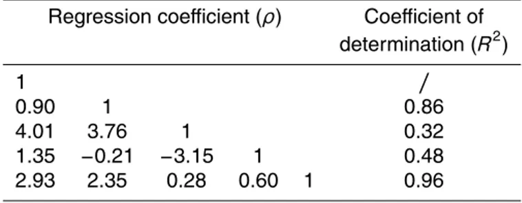
Figure 2 shows the cross-correlations of the five lumped aerosol emission species. With the exception of the auto-correlation in the diagonal line, all cross-correlations

5

exceed 0.5. This result reveals that the emission species are correlative, which may

be attributed to the common emission sources and diﬀ_{usion processes that are}

con-trolled by the same atmospheric circulation. The most significant cross-correlation is between E_EC and E_ORG with a value of approximately 0.8. This close correlation demonstrates that the emission distributions of these two species are very similar. Their

10

emissions are primary in urban and suburban areas with small emissions in rural areas and along roadways (not shown). As shown in Fig. 2, the lowest cross-correlation is be-tween E_ORG and E_SO4; the latter emissions are primary in the urban and suburban areas with few emissions in rural areas and roadways (not shown).

4 Balance constraints and BEC statistics

15

With the configuration of the WRF/Chem model described in Sect. 3.1, forecasts for one month (00:00 UTC of 15 May to 00:00 UTC of 14 June 2010) were performed

for the balance constraints and the BEC statistics. Forecast diﬀ_{erences between 24 h}

forecasts and 48 h forecasts are available at 00:00 UTC. Thirty forecast diﬀ_{erences are}

employed as inputs in the NMC method. For this method, 30 forecast diﬀ_{erences are}

20

suﬃ_{cient; however, a longer time series may be more beneficial for the BEC statistics}

(Parrish and Derber, 1992).

4.1 Balance regression statistics

Using these 30 forecast diﬀ_{erences, we can estimate the regression equations of EC,}

OC, NO3, SO4and OTR and calculate the unbalanced parts of these variables

(14)

GMDD

8, 10053–10088, 2015

assimilation

Z. Zang et al.

Title Page

Tables Figures

◭ ◮

Back Close

Full Screen / Esc

Discussion

P

a

per

|

Discussion

P

a

per

|

Discussion

P

a

per

|

Discussion

P

a

per

|

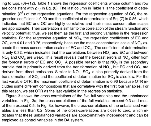
ing to Eqs. (6)–(12). Table 1 shows the regression coeﬃ_{cients whose column and row}

are consistent withρ_i_,_j in Eq. (6). The last column in Table 1 is the coeﬃ_{cient of}

deter-mination (R2) of the regression equations. For the regression equation of OC, the re-gression coeﬃ_{cient is 0.90 and the coe}ﬃ_{cient of determination of Eq. (7) is 0.86, which}

indicates that EC and OC are highly correlative and their mass concentration scales

5

are approximate. Their correlation is similar to the correlation of the stream function and velocity potential; thus, we set them as the first and second variables in the regression

statistics. For the regression equation of NO3, the regression coeﬃcients of EC and

OCuare 4.01 and 3.76, respectively, because the mass concentration scale of NO3

ex-ceeds the mass concentration scales of EC and OC_u. The coeﬃ_{cient of determination}

10

is only 0.32, which indicates that the correlations between NO3and EC and between

NO3 and OCu are weak. This result reveals that the forecast errors of NO3diﬀer from

the forecast errors of EC and OC_u. A possible reason is that NO₃ is the secondary

particle that is primarily derived from the transformation of NOx, but EC and OCu are

derived from direct emissions. Similar to NO3, SO4 is also primarily derived from the

15

transformation of SO₂and the coeﬃ_{cient of determination for SO}

4is also low. For the

last variable OTR, the maximum coeﬃ_{cient of determination is 0.96 because OTR}

in-cludes some diﬀ_{erent compositions that are correlative with the first four variables. For}

this reason, we set OTR as the last variable in the regression statistics.

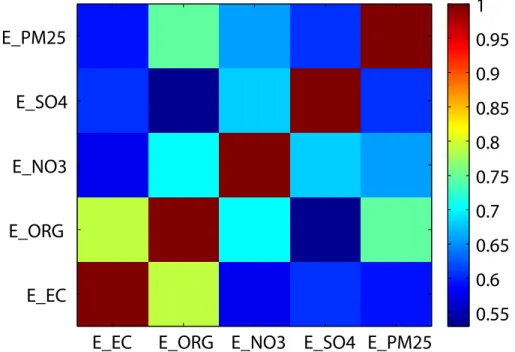
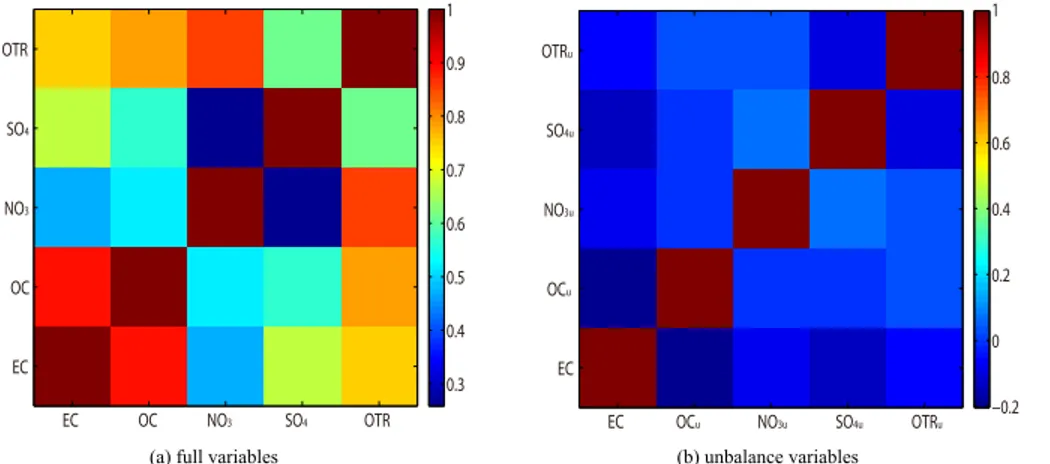
Figure 3 shows the cross-correlations of the five full variables and the unbalanced

20

variables. In Fig. 3a, the cross-correlations of the full variables exceed 0.3 and most of them exceed 0.5. In Fig. 3b, however, the cross-correlations of the unbalanced vari-ables are less than 0.2. Some of the cross-correlations are close to zero, which in-dicates that these unbalanced variables are approximatively independent and can be employed as control variables in the DA system.

(15)

GMDD

8, 10053–10088, 2015

assimilation

Z. Zang et al.

Title Page

Tables Figures

◭ ◮

Back Close

Full Screen / Esc

Discussion

P

a

per

|

Discussion

P

a

per

|

Discussion

P

a

per

|

Discussion

P

a

per

|

4.2 BEC statistics

Using the original full variables and the unbalanced variables obtained by the regres-sion equations, the BEC statistics are performed. Figure 2 shows the vertical profiles

of the standard deviations of the original D and the unbalanced D_u. In Fig. 2a, the

original standard deviation of NO3 is the largest value, whereas the smallest value is

5

OC, whose profile is close to the profile of EC. All profiles show a significant decrease at approximately 800 m because the aerosol particulates are usually limited under the boundary level. In Fig. 2b, all standard deviations significantly decrease, with the ex-ception of EC, which remains as the control variable in the unbalanced BEC statistics. Note that the standard deviation of OTR decreases by approximately 80 % compared

10

with NO3, which decreases by approximately 10 %. This result is attributed to the small

coeﬃ_{cient of determination for the regression of NO}₃_{(in Table 1), which indicates that}

a small portion of NO₃can be predicted by the regression and a large portion is an

un-balanced component. In contrast with NO3, a small portion of OTR is the unbalanced

component.

15

For the correlation matrix of C and C_u, they are factorized as three independent

one-dimensional correlation matrices in Eq. (21). The horizontal correlationCxorCyis

approximately expressed by a Gaussian function. The correlation between two points

r1andr2can be written ase

−(r2−r1)

2

2L2_s _{, where}_L

sis the horizontal correlation scale and is

a constant value forC_x and C_y, which are considered to be isotropic (Li et al., 2013).

20

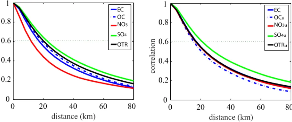
This scale can be estimated by the curve of the horizontal correlations with distances. Figure 5 shows the curves of the horizontal correlations for the five control variables. For the full variables (Fig. 5a), the sharpest decrease in the curves is observed for NO₃ and the slowest decrease in the curves is observed for SO4. The horizontal correlation

scales of EC, OC, NO3, SO4 and OTR are 25, 27, 20, 30 and 28 km, respectively.

25

For the unbalanced variables (Fig. 5b), their curves are closer than the curves of the

full variables. The correlation scales of EC, OC, NO3, SO4 and OTR are 25, 23, 24,

(16)

GMDD

8, 10053–10088, 2015

assimilation

Z. Zang et al.

Title Page

Tables Figures

◭ ◮

Back Close

Full Screen / Esc

Discussion

P

a

per

|

Discussion

P

a

per

|

Discussion

P

a

per

|

Discussion

P

a

per

|

expressed by common factors in the regression equations, which produces consistent horizontal correlation scales.

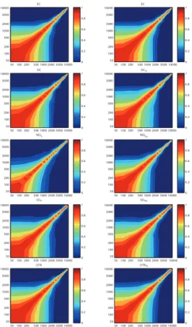
For the vertical correlation betweenCzandCuz, they are directly estimated using the

forecasting diﬀ_{erences because it is only an}_n

z×nz matrix. Figure 6 shows the vertical

correlation matricesCzandCuz for the full variables (left column) and the unbalanced 5

variables (right column), respectively. A common feature of both the full variables and the unbalanced variables is the significant correlation between the levels of the bound-ary layer height, which is consistent with the profile of the standard deviation in Fig. 4. Some weak adjustments to the correlations between the full and unbalanced variables are made. For example, the correlation of NO_3uis stronger than the correlation of NO₃

10

between the boundary layers, namely, the vertical correlation scale of NO_3u is larger

than the vertical correlation scale of NO3. Conversely, the vertical correlation scale of

OTRu is smaller than the vertical correlation scale of OTR. These results demonstrate

that the vertical correlations for the unbalanced variables are more consistent than the vertical correlations of the full variables, which is similar to the adjustments to the

15

horizontal correlation scale.

5 Application to data assimilation and prediction

To exhibit the eﬀ_{ect of the balance constraint of the BEC, the data assimilation}

ex-periments and 24 h forecasting are run using WRF/Chem model from 12:00 UTC on

3 June 2010 to 12:00 UTC on 4 June 2010. The surface PM2.5and aircraft-speciated

20

observations are assimilated using diﬀ_{erent BEC, and the evaluations are presented}

for the data assimilation and subsequent forecasts. Three basic statistical measures

in-cluding mean bias (BIAS), root mean square error (RMSE) and correlation coeﬃ_cient

(17)

GMDD

8, 10053–10088, 2015

assimilation

Z. Zang et al.

Title Page

Tables Figures

◭ ◮

Back Close

Full Screen / Esc

Discussion

P

a

per

|

Discussion

P

a

per

|

Discussion

P

a

per

|

Discussion

P

a

per

|

5.1 Observation data and experiment scheme

Two types of observation data are employed in our experiments. The first type of

obser-vation data consists of hourly surface PM2.5 concentrations, which are obtained from

the California Air Resources Board. A total of 42 surface PM_2.5 monitoring sites exist

in the innermost domain of the WRF/Chem model (Fig. 7). The second type of

obser-5

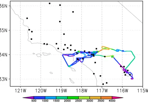
vation data is the speciated concentration along the aircraft flight track. The aircraft observations are investigated during the California Research at the Nexus of Air Qual-ity and Climate Change (CalNex) field campaign. This aircraft flight track is around Los Angeles from approximately 08:00 UTC on 3 June 2010 to 14:00 UTC on 3 June 2010 (Fig. 7). The species of the aircraft observations include OC, NO₃, SO₄and NH₄. Note

10

that NH4 is not a control variable; thus, the aircraft observations of NH4is disregarded

in the data assimilation. Because the particle size of the aircraft observations is less than 1.0 µm, some adjustments to the flight observations are made according to the ratios between the concentration under 2.5 µm and the concentration under 1.0 µm for each species using model products. With the ratios multiplied by the aircraft observed

15

concentrations, the speciated concentrations under 2.5 µm can be obtained.

Three parallel experiments are performed. The first experiment is the control ex-periment without aerosol data assimilation, which is frequently known as a free run and denoted as the control. The second experiment is a data assimilation experiment that assimilates surface PM2.5and aircraft observations using the full variables without

20

balance constraints; it is denoted as DA-full. The third experiment is also a data assim-ilation experiment that assimilates the same observations but employs the unbalanced variables as control variables conducted by the balanced constraint; it is denoted as DA-balance.

In each experiment, a 24 h forecasting is run using the WRf/Chem model with the

25

same configuration described in Sect. 3.1. These experiments begin from 12:00 UTC on 3 June 2010 and end at 12:00 UTC on 4 June 2010. For the DA-full and DA-balance

(18)

GMDD

8, 10053–10088, 2015

assimilation

Z. Zang et al.

Title Page

Tables Figures

◭ ◮

Back Close

Full Screen / Esc

Discussion

P

a

per

|

Discussion

P

a

per

|

Discussion

P

a

per

|

Discussion

P

a

per

|

aircraft-speciated observations from 10:30 to 13:30 UTC are assimilated for the use of more observation information.

5.2 Increments of data assimilation

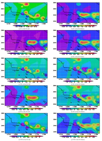
Figure 8 shows the horizontal increments of EC, OC, NO3, SO4 and OTR at the first

model level for the DA-full (left column) and DA-balance experiments (right column).

5

In the DA-full experiment, the increment of EC and OTR (Fig. 8a and i) are similar.

They are obtained from the surface PM2.5observations because no direct aircraft

ob-servations correspond to these two variables. In the DA-balance experiment, signif-icant adjustments are made to the increments of EC (Fig. 8b) under the action of the balance constraints. The same applies to the increment of OC (Fig. 8d) for their

10

high cross-correlation. Similarly, significant adjustments are made to the increment of OTR (Fig. 8j). The findings reveal some mixed characters of the first four variables

that are correlative with OTR. The increments of OC, NO3 and SO4 are aﬀected by

surface PM_2.5observations and aircraft observations. Some adjustments are made to

the value and horizontal scales of the increments. These results demonstrate that the

15

observation information can spread across variables by balance constraints.

Figure 9 shows the vertical increments along 35.0 N for the DA-full and DA-balance experiments. Similar to Fig. 8, the increments of EC and OTR (Fig. 9a and i) spread upward from the surface in the DA-full experiment, which are obtained from the surface

PM2.5 observation. In the DA-balance, the increments of EC and OTR (Fig. 9b and

20

j) exhibit observation information from the aircraft height at approximately 500 m, and the value of the increments show significant increases. The distributions of the incre-ments for these five variables in the DA-balance (Fig. 9, right column) generally tend to coincide compared with the distributions of the increments in the DA-full (Fig. 9, left column). The results of the DA-balance are reasonable due to the influence of each

25

(19)

GMDD

8, 10053–10088, 2015

assimilation

Z. Zang et al.

Title Page

Tables Figures

◭ ◮

Back Close

Full Screen / Esc

Discussion

P

a

per

|

Discussion

P

a

per

|

Discussion

P

a

per

|

Discussion

P

a

per

|

5.3 Evaluation of data assimilation and forecasts

Figure 10 shows the scatter plots of the model vs. the observed surface PM2.5 mass

concentrations at 12:00 UTC on 3 June 2010, which is the time of initialization. Com-pared with the control experiment, significant improvements in the evaluations of the DA-full are observed. The CORR increases by approximately 0.3. The RMSE and the

5

BIAS decrease approximately 50 % in the DA-full experiment (Fig. 10b). The evalua-tion of the DA-balance experiment (Fig. 10c) is similar to the evaluaevalua-tion of DA-full. The RMSE and BIAS of the DA-balance are slightly better than the RMSE and BIAS of DA-full, but the CORR of DA-balance is slightly lower than the CORR of DA-full. The main reason is probably attributed to the notion that the aircraft observations are

in-10

dependent of the surface observations and the adjustments of the balance constraints are primarily obtained from the speciated observations of the aircraft observations. These adjustments may not be consistent with the distribution of the surface

observa-tions. However, these minor diﬀ_{erences of statistical measures imply that the balance}

constraints in the DA-balance are reasonable, which does not destroy the primary

dis-15

tributions of the increments in DA-full.

Figure 11 shows the scatter plots of the model species vs. the aircraft observed species. The CORR of the DA-balance is the highest value of the three experiments during the total forecasting period (Fig. 1a). Note that the CORR in DA-balance and DA-full are similar prior to the first 3 h; however, the former is significantly higher than

20

(20)

GMDD

8, 10053–10088, 2015

assimilation

Z. Zang et al.

Title Page

Tables Figures

◭ ◮

Back Close

Full Screen / Esc

Discussion

P

a

per

|

Discussion

P

a

per

|

Discussion

P

a

per

|

Discussion

P

a

per

|

6 Summary and discussion

A set of balance constraints was established using a regression technique, which was incorporated in the BEC of a data assimilation system that is associated with

five control variables (EC, OC, NO₃, SO₄ and OTR) and is derived from the MOSAIC

aerosol scheme of the WRF/Chem model. Based on the NMC method, diﬀ_erences

5

within a month-long period between 24 and 48 h forecasts that are valid at the same time were employed in the estimation and analyses. For the original variables, these five control variables are highly correlative. Especially between EC and OC, their cor-relation is near 0.9. These original variables need to be transformed to satisfy the hypothesis of the independent control variables in the data assimilation system. We

10

employ the method of the balance constraint to divide the original full variables into balanced and unbalanced parts. The regression technique is used to express the bal-anced parts by the unbalbal-anced parts. Then, the independent unbalbal-anced parts are employed as control variables in the BEC statics. Accordingly, the standard deviations of these unbalanced variables are less than the standard deviations of the full variables.

15

The horizontal and vertical correlation scales of these unbalanced variables tend to be uniform for the eﬀ_{ect of the common factors in the regression equations.}

To evaluate the impact of the balance constraints on the analyses and forecasts, three parallel experiments, including a control experiment without data assimilation and two data assimilation experiments with and without balance constraints (DA-full

20

and DA-balance), were performed. In the data assimilation experiments, the same

ob-servations of surface PM_2.5 concentration and aircraft-speciated concentration of OC,

NO3and SO4were assimilated. The observations of these three variables can spread

to the two remaining variables in the increments of the DA-balance, which results in a more complicated distribution with more local centers. Even for the area with only

25

surface PM_2.5 observations, some adjustments in the increments of the DA-balance

are made for the mutual spread across variables compared with the increments of the

(21)

GMDD

8, 10053–10088, 2015

assimilation

Z. Zang et al.

Title Page

Tables Figures

◭ ◮

Back Close

Full Screen / Esc

Discussion

P

a

per

|

Discussion

P

a

per

|

Discussion

P

a

per

|

Discussion

P

a

per

|

two data assimilation analysis fields when we evaluated them using the surface PM_2.5

observations with the statistical measures of CORR, RMSE and BIAS. However, these

diﬀ_{erences are minor because the surface PM}_2.5 _{observations are independent of the}

aircraft observations and the balance constraints cannot break the primary balance of the species.

5

The incorporation of the balance constraints improves the initial DA analysis fields. During the subsequent forecasts until 24 h, the improvements are more significant for the evaluation of the balance experiment compared with the evaluation of the DA-full experiment, especially from the 3rd hour to the 18th hour. These results suggested that the balance constraint can optimize the initial distribution of variables. Although

10

the optimization is slight for the initial analysis fields, it can serve an import role for improving the skill of sequent forecasts.

The method for incorporating balance constraints in aerosol data assimilation can

be employed in other areas or other applications for diﬀ_{erent aerosol models. For the}

aerosol variables in diﬀ_{erent models, some cross-correlations should exist because}

15

their common emissions and diﬀ_{usion processes are controlled by the same}

atmo-spheric circulation. Although these correlations may be stronger than the cross-correlations of atmospheric or oceanic model variables, theoretic balance constraints, such as geostrophic balance or temperature-salinity balance, do not exist. We expected to discover a universal balance constraint among the aerosol variables and utilize it in

20

the data assimilation system. In addition, we expected to expand the balance constraint to include gaseous pollutants, such as nitrite (NO2), sulfur dioxide (SO2), and (carbon

monoxide) CO. These gaseous pollutants are correlative with some aerosol species,

such as NO3, SO4 and EC, which can improve the data assimilation analysis fields

of aerosols by assimilating these gaseous observations. The assimilation of aerosol

25

observations may improve the analysis fields of gaseous pollutants.

(22)

GMDD

8, 10053–10088, 2015

assimilation

Z. Zang et al.

Title Page

Tables Figures

◭ ◮

Back Close

Full Screen / Esc

Discussion

P

a

per

|

Discussion

P

a

per

|

Discussion

P

a

per

|

Discussion

P

a

per

|

Sciences Division (http://esrl.noaa.gov/csd/groups/csd7/measurements/2010calnex/), for pro-viding the download of surface and aircraft aerosol observations.

References

Bannister, R. N.: A review of forecast error covariance statistics in atmospheric variational data assimilation. I: Characteristics and measurements of forecast error covariances, Q. J. Roy.

5

Meteorol. Soc., 134, 1951–1970, 2008a.

Bannister, R. N.: A review of forecast error covariance statistics in atmospheric variational data assimilation. II: Modelling the forecast error covariance statistics, Q. J. Roy. Meteorol. Soc., 134, 1971–1996, 2008b.

Barker, D. M., Huang, W., Guo, Y.R, and Xiao, Q. N.: A Three-Dimensional (3DVAR) data

as-10

similation system for use with MM5: implementation and initial results, Mon. Weather Rev., 132, 897–914, 2004.

Benedetti, A. and Fisher, M.: Background error statistics for aerosols, Quart. J. Roy. Meteor. Soc., 133, 391–405, 2007.

Chen, Y., Rizvi, S., Huang, X., Min, J., and Zhang, X.: Balance characteristics of multivariate

15

background error covariances and their impact on analyses and forecasts in tropical and Arctic regions, Meteorol. Atmos. Phys., 121, 79–98, 2013.

Cohn, S. E.: Estimation theory for data assimilation problems: basic conceptual framework and some open questions, J. Meteorol. Soc. Jpn., 75, 257–288, 1997.

Derber, J. and Bouttier, F.: A reformulation of the background error covariance in the ECMWF

20

global data assimilation system, Tellus, 51, 195–221, 1999.

Grell, G. A., Peckham, S. E., Schmitz, R., McKeen, S. A., Frost, G., Skamarock, W. C., and Eder, B.: Fully coupled “online” chemistry within the WRF model, Atmos. Environ., 39, 6957– 6976, doi:10.1016/j.atmosenv.2005.04.027, 2005.

Guenther, A., Karl, T., Harley, P., Wiedinmyer, C., Palmer, P. I., and Geron, C.: Estimates

25

(23)

GMDD

8, 10053–10088, 2015

assimilation

Z. Zang et al.

Title Page

Tables Figures

◭ ◮

Back Close

Full Screen / Esc

Discussion

P

a

per

|

Discussion

P

a

per

|

Discussion

P

a

per

|

Discussion

P

a

per

|

Hoek, G., Meliefste, K., Cyrus, J., Lewne, M., Bellander, T., Brauer, M., Fischer, P., Gehring, U., Heinrich, J., van Vliet, P., and Brunekreef, B.: Spatial variability of fine particle concentrations in three European areas, Atmos. Environ., 36, 4077–4088, 2002.

Huang, X. Y., Xiao, Q., Barker, D. M., Zhang, X., Michalakes, J., Huang, W., and Henderson, T.: Four-dimensional variational data assimilation for WRF: formulation and preliminary results,

5

Mon. Weather Rev., 137, 299–314, 2009.

Jazwinski, A. H.: Stochastic Processes and Filtering Theory, Academic Press, New York, 376 pp., 1970.

Kahnert, M.: Variational data analysis of aerosol species in a regional CTM: background er-ror covariance constraint and aerosol optical observation operators, Tellus B, 60, 753–770,

10

2008.

Li, Z., Zang, Z., Li, Q. B., Chao, Y., Chen, D., Ye, Z., Liu, Y., and Liou, K. N.: A three-dimensional variational data assimilation system for multiple aerosol species with WRF/Chem and an

application to PM_2.5 prediction, Atmos. Chem. Phys., 13, 4265–4278,

doi:10.5194/acp-13-4265-2013, 2013.

15

Liu, Z., Liu, Q., Lin, H. C., Schwartz, C. S., Lee, Y. H., and Wang, T.: Three-dimensional varia-tional assimilation of MODIS aerosol optical depth: implementation and application to a dust storm over East Asia, J. Geophys. Res., 116, D23206, doi:10.1029/2011JD016159, 2011. Mesinger, F., DiMego, G., Kalnay, E., Shafran, P., Ebisuzaki, W., Jovic, D., Woollen, J.,

Mitchell, K., Rogers, E., Ek, M., Fan, Y., Grumbine, R., Higgins, W., Li, H., Lin, Y., Manikin, G.,

20

Parrish, D., and Shi, W.: North American regional reanalysis, B. Am. Meteorol. Soc., 87, 343– 360, 2006, 2013.

Pagowski, M., Grell, G. A., McKeen, S. A., Peckham, S. E., and Devenyi, D.: Three-dimensional variational data assimilation of ozone and fine particulate matter observations: some results using the Weather Research and Forecasting–Chemistry model and Grid-point Statistical

25

Interpolation, Q. J. Roy. Meteor. Soc., 136, 2013–2024, doi:10.1002/qj.700, 2010.

Parrish, D. F. and Derber, J. C.: The national meteorological center spectral statistical interpo-lation analysis, Mon. Weather Rev., 120, 1747–1763, 1992.

Peckam, S. E., Grell, G. A., McKeen, S. A., and Ahmadov, R.: WRF/Chem Version 3.5 User’s Guide, NOAA Earth System Research Laboratory, Colorado, 2013.

30

(24)

GMDD

8, 10053–10088, 2015

assimilation

Z. Zang et al.

Title Page

Tables Figures

◭ ◮

Back Close

Full Screen / Esc

Discussion

P

a

per

|

Discussion

P

a

per

|

Discussion

P

a

per

|

Discussion

P

a

per

|

Saide, P. E., Carmichael, G. R., Spak, S. N., Minnis, P., and Ayers, J. K.: Improving aerosol distributions below clouds by assimilating satellite-retrieved cloud droplet number, P. Natl. Acad. Sci. USA, 109, 11939–11943, doi:10.1073/pnas.1205877109, 2012.

Saide, P. E., Carmichael, G. R., Liu, Z., Schwartz, C. S., Lin, H. C., da Silva, A. M., and Hyer, E.: Aerosol optical depth assimilation for a size-resolved sectional model: impacts of

obser-5

vationally constrained, multi-wavelength and fine mode retrievals on regional scale analy-ses and forecasts, Atmos. Chem. Phys., 13, 10425–10444, doi:10.5194/acp-13-10425-2013, 2013.

Salako, G. O., Hopke, P. K., Cohen, D. D., Begum, B. A., Biswas, S. K., Pandit, G. G., Chung, Y. S., Rahman, S. A., Hamzah, M. S., Davy, P., Markwitz, A., Shagjjamba, D.,

10

Lodoysamba, S., Wimolwattanapun, W., and Bunprapob, S.: Exploring the variation between EC and BC in a variety of locations, Aerosol Air Qual. Res, 12, 1–7, 2012.

Schwartz, C. S., Liu, Z., Lin, H. C., and McKeen, S. A.: Simultaneous three-dimensional vari-ational assimilation of surface fine particulate matter and MODIS aerosol optical depth, J. Geophys. Res., 117, D13202, doi:10.1029/2011JD017383, 2012.

15

(25)

GMDD

8, 10053–10088, 2015

assimilation

Z. Zang et al.

Title Page

Tables Figures

◭ ◮

Back Close

Full Screen / Esc

Discussion

P

a

per

|

Discussion

P

a

per

|

Discussion

P

a

per

|

Discussion

P

a

per

|

Table 1. Regression coeﬃ_{cients of balance operator K and the coe}ﬃ_{cient of determination}

(regression coeﬃ_{cients correspond to}_ρ

ijin Eq. 6).

Regression coeﬃ_{cient (}_ρ₎ _Coeﬃ_{cient of}

determination (R2)

1 /

0.90 1 0.86

4.01 3.76 1 0.32

1.35 −0.21 −3.15 1 0.48

(26)

GMDD

8, 10053–10088, 2015

assimilation

Z. Zang et al.

Title Page

Tables Figures

◭ ◮

Back Close

Full Screen / Esc

Discussion

P

a

per

|

Discussion

P

a

per

|

Discussion

P

a

per

|

Discussion

P

a

per

|

136W

128W 120W 112W 104W

96W

30N

35N

40N

45N

50N

d01

d03

Los Angeles

d02

Figure 1. Geographical display of the three-nested model domains. The innermost domain

(27)

GMDD

8, 10053–10088, 2015

assimilation

Z. Zang et al.

Title Page

Tables Figures

◭ ◮

Back Close

Full Screen / Esc

Discussion

P

a

per

|

Discussion

P

a

per

|

Discussion

P

a

per

|

Discussion

P

a

per

|

E_EC

E_ORG E_NO3 E_SO4 E_PM25

E_EC

E_ORG

E_NO3

E_SO4

E_PM25

0.55

0.6

0.65

0.7

0.75

0.8

0.85

0.9

0.95

1

Figure 2.Cross-correlations between emission species of E_EC, E_ORG, E_NO3, E_SO4 and

(28)

GMDD

8, 10053–10088, 2015

assimilation

Z. Zang et al.

Title Page

Tables Figures

◭ ◮

Back Close

Full Screen / Esc

Discussion

P

a

per

|

Discussion

P

a

per

|

Discussion

P

a

per

|

Discussion

P

a

per

|

EC OC NO3 SO4 OTR

EC OC NO3

SO4

OTR

0.3 0.4 0.5 0.6 0.7 0.8 0.9 1

(a) full variables

EC OCu NO3u SO4u OTRu

EC OCu

NO3u

SO4u

OTRu

−0.2 0 0.2 0.4 0.6 0.8 1

(b) unbalance variables

Figure 3.Cross-correlations between the five variables of the BEC. These variables are(a)full

(29)

GMDD

8, 10053–10088, 2015

assimilation

Z. Zang et al.

Title Page

Tables Figures

◭ ◮

Back Close

Full Screen / Esc

Discussion

P

a

per

|

Discussion

P

a

per

|

Discussion

P

a

per

|

Discussion

P

a

per

|

0 0.1 0.2 0.3 0.4 0.5

50 100 200 500 1000 2000 5000 10000

standard deviation ( µg/m 3 )

height (m)

0 0.1 0.2 0.3 0.4 0.5

50 100 200 500 1000 2000 5000 10000

standard deviation ( µg/m 3 )

height (m)

(a) full variables (b) unbalanced variables

EC OC NO3

SO4

OTR

EC OCu

NO3u

SO4u

OTRu

(30)

GMDD

8, 10053–10088, 2015

assimilation

Z. Zang et al.

Title Page

Tables Figures

◭ ◮

Back Close

Full Screen / Esc

Discussion

P

a

per

|

Discussion

P

a

per

|

Discussion

P

a

per

|

Discussion

P

a

per

|

0 20 40 60 80 0

0.2 0.4 0.6 0.8 1

distance (km)

correlation

0 20 40 60 80 0

0.2 0.4 0.6 0.8 1

distance (km)

correlation

EC

OC

NO3

SO4

OTR

EC

OCu

NO3u

SO4u

OTRu

Figure 5.Same as Fig. 3, with the exception of the horizontal auto-correlation curves of the